Demystifying the Transferability of Adversarial Attacks in Computer Networks

Abstract

Convolutional Neural Networks (CNNs) models are one of the most frequently used deep learning networks, and extensively used in both academia and industry. Recent studies demonstrated that adversarial attacks against such models can maintain their effectiveness even when used on models other than the one targeted by the attacker. This major property is known as transferability, and makes CNNs ill-suited for security applications.

In this paper, we provide the first comprehensive study which assesses the robustness of CNN-based models for computer networks against adversarial transferability. Furthermore, we investigate whether the transferability property issue holds in computer networks applications. In our experiments, we first consider five different attacks: the Iterative Fast Gradient Method (I-FGSM), the Jacobian-based Saliency Map (JSMA), the Limited-memory Broyden Fletcher Goldfarb Shanno BFGS (L-BFGS), the Projected Gradient Descent (PGD), and the DeepFool attack. Then, we perform these attacks against three well-known datasets: the Network-based Detection of IoT (N-BaIoT) dataset, the Domain Generating Algorithms (DGA) dataset, and the RIPE Atlas dataset. Our experimental results show clearly that the transferability happens in specific use cases for the I-FGSM, the JSMA, and the LBFGS attack. In such scenarios, the attack success rate on the target network range from 63.00% to 100%. Finally, we suggest two shielding strategies to hinder the attack transferability, by considering the Most Powerful Attacks (MPAs), and the mismatch LSTM architecture.

I Introduction

In the 21st century, the evolution of artificial intelligence has demonstrated the tremendous benefit of deep learning algorithms to solve the most challenging problems of our society [1]. For example, applying deep learning techniques in the medical field shows promising results to perfectly detect and classify cancerous tissues through histopathology images [2]. Nowadays, existing Neural Networks (NNs) solutions have achieved human-level performance. In particular, Convolutional Neural Networks (CNNs) models which are among the most popular neural network architectures. Convolutional Neural Networks (CNNs) are increasingly employed in various computer network applications, such as network threat detection, network intrusion detection [3], malware detection in 5G-IoT Healthcare Applications [4], and multimedia forensics to detect several distorted pictures [5]. Prior studies investigated the robustness of Graph Neural Networks against adversarial attacks[6], and demonstrated the possibility of successfully identifying important patterns of adversarial attacks against such networks. In this line of research, the fundamental issue is that even when only partial information of the graph is provided, or the attack is limited to a few perturbations, the classification performance constantly degrades. Furthermore, the attacks apply to a variety of node categorization schemes. As a result, the CNN model outperforms Graph Neural Networks regarding classification performance.

On the other hand, recent research studies have shown that some examples can be precisely computed to mislead machine-learning models [7]. To better illustrate these examples, Grosse et al. [8] proved the possibility of crafting Android malware examples to mislead neural network malware detection models. The authors adapted the algorithm proposed by Papernot et al. [9] to craft the adversarial samples. More specifically, the proposed crafting algorithm utilizes the Jacobian matrix of the neural network.

To elaborate more, the generation of these examples are so-called adversarial examples and pose real-life security threats [10]. A real-world scenario consists of making a self-driving car misclassify the red light as green. This scenario could be a life-threatening example for autonomous vehicles. The popularity and diversity of the CNN applications make them a perfect target for adversarial examples. The concept of adversarial examples was introduced in 2014 by Szegedy et al. [11]. Later, many studies demonstrated the use of different adversarial attacks to compromise CNN-based models (e.g., offline handwritten signature verification, synthetic aperture radar image classification, object detection, automatic speech recognition). These attacks pose new security threats for systems built on machine learning algorithms, hindering the model’s functionality in various applications.

It is worth mentioning that building adversarial examples can typically be applied to every machine learning algorithm due to the native characteristics of machine learning architectures. This vulnerability also affects modern deep neural networks. An interesting case in a black-box setting is that two models with different network architectures and trained with different training sets can misclassify the same adversarial example. In this scenario, the adversary trains the source network, and designs the adversarial example, then transfer it to the victim’s network even with a few knowledge about the victim’s model [12]. This substantial property is known as transferability and might disrupt CNN’s operation in various applications. To better visualize this concept, Wu et al. [13] evaluated the adversarial transferability in image classification against three datasets (MNIST, CIFAR-10, and ImageNet) and provided three key factors influencing it: the architecture, the test accuracy, and the model capacity. For the architecture, the similarity between the source and target model significantly enables the transferability property. Regarding the test accuracy, the models with high accuracy manifest high transferability. However, the models with deeper capacity (i.e., higher amount of model parameters) are less transferable when they act as source models.
The purpose of our study is to see if and to what degrees the transferability of adversarial examples applies in computer networks, following some recent studies demonstrating that adversarial examples jeopardize CNN forensics techniques [14]. From a research point of view, it is highly important to answer this question because the attack transferability would make developing defense strategies much more complex. Furthermore, giving the attacker a complete access to the source network will not prevent fooling the target network. Experimental evidence demonstrated by Tramèr et al. [15] has shown that the transferability of adversarial examples from a source network to a target network is more likely to occur in very large adversarial subspaces (i.e., the space of adversarial examples), where the two models will intersect. Consequently, the subspace dimensionality of two adversarial subspaces correlates with the transferred property.
In this paper, we solely consider two instances of CNN’s deep learning networks, which have lately been employed in computer vision, multimedia forensics, adversarial machine learning, and other fields. We mainly investigate if the attack transferability might occur in security-oriented applications for computer networks. In other words, we verify if an adversarial attack on a Source Network (SN) might be effective against a possibly different and unknown Target Network (TN). Although authors in [14, 12] recently demonstrated that the transferability of adversarial samples holds in computer vision applications and computer forensics. We launched five different attacks against three well-known datasets under black-box settings. Our experimental results demonstrate that the generated adversarial examples are not transferable in most cases. However, just a few cases of attacks are transferable from the SN to the TN. In particular, in the cross model transferability scenario where the same datasets such as N-BaIoT, DGA, and RIPE Atlas datasets are trained on two different network architectures. These adversarial examples achieve good transferability and can perfectly deceive the TN.

I-A Contributions

Our contributions are summarized as follows:

• We offer the FAIL models SPRITZ1 and SPRITZ2 that fails against different adversarial attacks, and which provides a basic framework for simulating and analyzing realistic adversaries. Across multiple degrees of adversarial control, we assess the robustness of the networks in terms of attack transferability against machine learning systems.

• We perform five different adversarial attacks with different parameters from low to high to demystify the transferability in computer networks, namely: the I-FGSM attack, the JSMA attack, the L-BFGS attack, the PGD attack, and the DeepFool attack.

• We independently examine the impact of training data and network architecture mismatch on the attacks’ transferability. Furthermore, we systematically investigate the impact of partial adversarial knowledge and control on the robustness of machine learning models against the test-time attack (exploratory evasion-attack).

• We offer two shielding strategies that overcome prior adversarial attacks’ limits. First, by using mismatch classifiers and considering the LSTM architecture as a target network to hinder the adversarial transferability. Second, by fine-tuning with Most Powerful Attacks (MPAs) [16] to improve the security of the target network.

I-B Organization

We outline the rest of our paper as follows. In Section II, we provide the background and preliminaries on the datasets and adversarial attacks used in our experiments. Then, we overview the related works that discussed the transferability property in Section III. Afterward, in Section IV, we provide our methodology and the experimental setup. Section V presents the experimental results followed by a discussion evaluating the transferability in computer networks, and presents two recent approaches for hindering adversarial transferability. Finally, we conclude our paper and provide promising future research work in Section VI.

II Background

In this section, we provide the background on the datasets and adversarial attacks used in our experiments. First, we present the N-BaIoT [17], the DGA [18], and RIPE Atlas[19] datasets. Afterward, we discuss the adversarial attacks performed to evaluate the transferability property in CNN-based models on computer networks. Table I lists all the abbreviations and notations used in our paper.

Table I: Abbreviation and Notation List.

Acronym	Description
CNN	Convolutional Neural Network
LSTM	Long Short-Term Memory Networks
LK	Limited Knowledge
PK	Perfect Knowledge
CF	Counter Forensics
DL, ML	Deep Learning, Machine Learning
SN, TN	Source Network, Target Network
CM	Cross Model
CT	Cross Training
CMT	Cross Model and Training
ASR	Average Attack Success Rate
Max. dist	Average Maximum distortion
PSNR	Average Peak signal-to-noise ratio
$L_{1}$ dist	Average $L_{1}$ distance
FGSM	Fast Gradient Sign Method
I-FGSM	Iterative Fast Gradient Sign Method
JSMA	Jacobian-based Saliency Map Attack
LBFGS	Limited-memory Broyden-Fletcher-Goldfarb-Shanno
PGD	Projected Gradient Descent
N-BaIoT	Network-based Detection of IoT
DGA	Domain Generating algorithms
DN	Domain Name
RNN	Recurrent Neural Network
DDoS	Distributed Denial of Service

II-A Datasets

To evaluate the effectiveness of the transferability property in computer networks, we considered comprehensive real-world datasets that contain malicious and benign data in computer networks. It is worth mentioning the importance of relying on the high quality of datasets to achieve high training accuracy [20]. In our experiments, we train the SN and the TN on three different datasets, namely: the N-BaIoT, the DGA, and the RIPE Atlas datasets. Additionally, these datasets are well-known and have lately been used for various cybersecurity purposes. The N-BaIoT dataset has been used to recognize botnet attacks in IoT devices employing deep auto-encoders [21], detection methods in the Internet of Things [22], and federated learning for detecting attacks in the Internet of things [23]. Besides, the DGA dataset is one of the most widely used datasets in detecting and classifying DGA botnets, and their families [24]. It presents a framework to identify Domain Generating Algorithms (DGAs) in real-world network traffic [18]. The RIPE Atlas dataset has been employed in JurisNN [25], network devices monitor and alerts [26], and so forth. In what follows, we provide a detailed description of each one of the considered datasets.

II-A1 N-BaIoT datasets

The N-BaIoT datasets are built upon the collection of real benign and malicious traffic using port mirroring techniques and gathered from nine different commercial IoT devices. The N-BaIoT datasets contain 115 features and around seven million instances. With the increase of the IoT cyber attacks, which turns out the Internet of Things into the internet of vulnerabilities, the adversaries rely on using botnets to exploit such vulnerabilities [27]. The generation of malicious IoT traffic for the N-BaIoT datasets is performed by compromising nine commercial devices by two well-known IoT-based botnets: The BASHLITE botnet and the Mirai botnet. These botnets leverage the use of DDoS (Distributed Denial of Service) attack resulting in the unavailability of the IoT devices. The BASHLITE botnet is a well-known IoT botnet that infects Linux-based IoT devices. With its capability of launching DDoS attacks, BASHLITE infected up to 1 million IoT commercial devices, mostly DVRs and web-connected video cameras [28]. The Mirai botnet is one of the most popular IoT botnets that infected thousands of devices used in the past decades. The release of its source code shows that Mirai botnet consists of (1) automatic scanning for vulnerable IoT devices, (2) uploading the malware into the vulnerable IoT device to perform the DDoS attack. The cyber attacks performed by the two authentic botnets in the IoT network cover flooding attacks (e.g., TCP-SYN flooding attack, UDP flooding attack), sending spam data, and scanning attacks.

The collection of malicious traffic generated by such attacks supports the adoption of N-BaIoT datasets in several applications. In [21], the authors provided a deep learning network-based anomaly detection method for IoT botnets. Their experimental results show that the use of deep autoencoders techniques can accurately detect IoT botnets. Another work proposed a privacy-preserving framework for malware detection in IoT devices [23], the authors applied federated learning mechanisms for training and evaluating supervised and unsupervised learning models while protecting the privacy of sensitive shared data. We believe that we can also consider deep autoencoders approach utilized for IoT botnet detection to investigate the transferability property.

II-A2 DGA datasets

The DGA datasets comprise legitimate and malicious DNs (Domain Names). The clean datasets are the Alexa (1M) records of top websites [18], and the malicious DNs are gathered from more than 25 different families of malware (e.g., Kraken, nymaim, shiotob, and alureon) that exploit the DGA algorithm. These algorithms are embedded into the malware and principally designed to generate many malicious DNs automatically. In addition, DGA algorithms are resistant against blacklisting and sinkholing techniques, which detect and block malicious DNs. Integrating DGA algorithms into the malware enables C&C (Command and Control) servers for botnets to perform potential DDoS attacks. Given the high quality and practical applications of DGA datasets, prior works in the literature have considered the DGA datasets. In [29], the authors developed an approach to detect DGA-based malware. This approach enables the identification of a single DGA domain and relies on using a set of lexical evidence and RF (Random forest) algorithms to profile DGA-based malware. A similar work investigated the use of DL algorithms to detect DGAs [30], the authors leveraged the RNN based architectures to detect potentially malicious DGAs, and their evaluation on real-world dataset demonstrated the high performance of RNN based DGA classifiers.

II-A3 RIPE Atlas datasets

The Internet of Things (IoT) concept has acquired much interest in past years. One approach to characterize IoT networks is through a large collection of Internet-aware detectors and controllers, including the electrical switches that turn the central air conditioning device on or off. The RIPE Atlas study assesses information about the Network through Internet-aware sensors [19]. RIPE Atlas could also be used to continually check the accessibility of networks or hosts from hundreds of locations across the world. Additionally, it can perform ad hoc connection tests to analyze and resolve identified network issues and test the availability of DNS servers. In these datasets, we considered feature-engineered RAW data by decoding the buffers returned in DNS queries, and returning the DNS measurement results [31]. Initially, the RIPE dataset aim to identify the application’s type based on the flow data. These datasets are tested in two different network architectures: the Recurrent Neural Networks (RNN), and the Convolutional Neural Networks (CNN). We mention that several transformation steps have been performed to prepare the datasets [32], and the network is trained to classify the flow sequence for several applications. Although the accuracy of both training and testing data reached 80%, the model can perfectly predict the majority of flow sequences, and the error rate is significantly reduced by feeding additional data into the system.

II-B Adversarial Attacks

Much attention has been received recently concerning the possibility of adversarial examples to fool the CNN-based models. In the existing literature, the adversary can perform the adversarial attack under three different settings: (i) white-box, (ii) gray-box, and (iii) black-box attacks. (i) In the white-box setting, the adversary has a Perfect Knowledge (PK) on the TN by adopting a particular categorization for adversarial examples [10]. (ii) In the gray-box setting, the adversary has a Limited Knowledge (LK) on the TN [33]. (iii) In the black-box setting, the attacker does not have access to the internal details of the TN, which is a more feasible and complicated scenario than the previous ones; as a result, the adversary uses multiple queries to obtain such internal details. Therefore, we are motivated to consider the black-box scenario given its feasibility in real-world applications. In our study, we propose and test a generalized technique for black-box threats on ML that takes advantages of adversarial transferability.

In our work, we performed five adversarial attacks under black-box settings, where we do not have access to the underlying deployed model: The I-FGSM attack [34], the JSMA attack [9], the L-BFGS attack [11], the PGD attack [35], and the DeepFool attack [36]. In our experiments, we considered the Foolbox library [37] to implement all adversarial attacks.

II-B1 The I-FGSM attack

The I-FGSM attack represents the iterative version of the FGSM (Fast Gradient Sign Method) [38]. The FGSM attack is one of the most well-known adversarial examples. It consists of targeting neural networks, which fails the network and potential misclassification of an input. The Fast Gradient Sign Method is a gradient-based attack that adjusts the input data to maximize the loss. Given an input $X$ of a model with $\theta$ parameters and a ground truth label $Y$. We compute the adversarial example $Adv_{X}$ of the FGSM attack as follows:

$$Adv_{X}=X+\epsilon\times sign(\triangledown_{X}J(\theta,X,Y)).$$ (1)

Where $\epsilon$ is the normalized attack strength factor, and $J$ is the cross-entropy cost function used to train the model. We mention that $\epsilon$ is the parameter controlling the perturbations and should be considered minimal for the success of the adversarial example. Given that the FGSM attack often fails in some scenarios, the iterative version of the FGSM attack, namely the I-FGSM attack [34], guarantees finer perturbations and could be described as a straightforward extension of the FGSM. More specifically, the I-FGSM attack considers iterating the FGSM method with smaller steps on the way to the gradient sign. For the I-FGSM attack, we express the adversarial example for each $i+1$ iteration such that $Adv^{0}_{X}=X$ as follows:

$$Adv^{i+1}_{X}=Adv^{i}_{X}+\epsilon*sign(\triangledown_{X}J(\theta,Adv^{i}_{X},Y)).$$ (2)

II-B2 The JSMA attack

Papernot et al. [9] introduced the JSMA attack to reduce the number of perturbations comparing to the I-FGSM attack. Therefore, the construction of JSMA-based adversarial examples is more suitable than I-FGSM for targeted misclassification and harder to detect. However, the JSMA algorithm requires a high computational cost. The JSMA attack is a gradient-based method that uses a forward derivative approach and adversarial saliency maps. Instead of a backward propagation like the I-FGSM attack, the forward derivative is an iterative procedure that relies on forward propagation. Given an $N$-dimensional input $X$ of a model, the adversary starts by computing a Jacobian matrix of the $M$-dimensional classifier $F$ learned by the model during the training phase. The Jacobian matrix is given by:

$$J_{F}(X)=\partialderivative{F(X)}{X}={\begin{bmatrix}\partialderivative{F_{j}(X)}{x_{i}}.\end{bmatrix}}_{i\in 1..M,j\in 1..N}.$$ (3)

Afterward, the adversary produces adversarial samples by constructing the adversarial saliency maps $S$ based on the forward derivative. These maps identify specific input features where the adversary enables the perturbations needed for the desired output. Thus, building the adversarial sample space. For a target class $t$, we define the adversarial saliency map by the following equation:

$$S(X,t)[i]=\left\{\begin{array}[]{ll}0,if\frac{\partial F_{t}}{\partial x_{i}}(X)<0\text{ or }\sum_{j\neq t}\frac{\partial F_{j}}{\partial x_{i}}(X)>0.&\\ {\frac{\partial F_{t}}{\partial x_{i}}(X)\left|\sum_{j\neq t}\frac{\partial F_{j}}{\partial x_{i}}(X)\right|,}otherwise.&\end{array}\right.$$ (4)

In summary, JSMA is a greedy repeated process that generates a saliency map at each iteration through forwarding propagation, indicating which pixels contributed the most to classification. A large value in this map, for instance, indicates that changing that pixel significantly increases the likelihood of selecting the incorrect class. The pixels are then changed individually, depending on this map, by a relevant number $\theta$ ($\theta$ refers to the range of possible pixel changes).

II-B3 The L-BFGS attack

The L-BFGS attack has been proposed by Szegedy et al. [11]. It is a non-linear gradient-based numerical optimization method and aims to reduce the perturbations for a given input. The L-BFGS attack generates the adversarial examples by optimizing the input $X$ and maximizing the prediction error. The L-BFGS attack is a practical box-constrained optimization method to generate adversarial samples. However, it is time-consuming and computationally demanding. For an input $X$, The formal expression of the optimization problem of the L-BFGS attack is given by:

$$\min_{Adv_{X}}||X-Adv_{X}||^{2}_{2}\mbox{ subject to: }F(X+r)=l.$$ (5)

Such that $F$ is the classifier, $l$ is the target label, and $r$ is the minimizer. However, the optimization problem depicted in Eq. 5 is computationally expensive and considered as a hard problem. An approximate solution solves this problem by using a box-constrained L-BFGS [11], and is expressed as follows:

$$\min_{Adv_{X}}c.||X-Adv_{X}||^{2}_{2}-J(\theta,X,Y).$$ (6)

In this approximation, the objective is to find the minimum scalar $c>0$ and for which the minimizer $r$ of the Eq. 5 is satisfied.

II-B4 The PGD attack

The PGD attack [35] is a first-order adversarial attack, i.e., consists of using the local first-order information about the targeted network. It is an iterative version of the FGSM, such as the I-FGSM. Except that in the PGD attack, for each iteration $i+1$, the input $X$ is updated according to the following rule:

$$Adv^{i+1}_{X}=\Pi_{X+S}(Adv^{i}_{X}+\epsilon*sign(\triangledown_{X}J(\theta,X,Y))).$$ (7)

Where $\Pi$ is the projection operator that keeps $Adv^{i+1}_{X}$ within a set of perturbation range $S$. We note that the PGD attack looks for the perturbations that maximize $J(\theta,X,Y)$ while considering the $L^{\infty}$ distortion.

II-B5 The DeepFool attack

Regarding the DeepFool attack [36], it fools the binary and multiclass classifiers by finding the closest distance from the input $X$ to the other side of the classification boundary. For any given classifier, the minimal perturbation $r$ to generate an adversarial example by the DeepFool attack is formally expressed by:

$$\delta(X,F)=\min_{r}||r||_{2}\mbox{ subject to: }F(X+r)\neq F(X).$$ (8)

Such that $\delta$ describes the robustness of $F$ at the input $X$. We mention that the state-of-the-art classifiers are weak against the DeepFool attack. Therefore, the DeepFool present a reference to test and evaluate the robustness and the performance of existing classifiers. The N-BaIoT datasets are built open the collection of real and benign malicious traffic in pcap using nine gathered

III Related Work

The early studies of adversarial examples revealed the transferability of adversarial attacks [38, 11]. Recently, initial efforts have been devoted to explore this property in different areas (e.g., multimedia forensics, natural language processing).

In multimedia forensics applications, the use of machine learning techniques offers promising solutions for security analysts. However, adversarial image forensics significantly hinder such possibility [7]. Barni et al. [39] investigated the transferability of adversarial examples in CNN-based models. The authors launched the I-FGSM and the JSMA attacks against two different datasets and argued that adversarial examples are non-transferable under black-box settings. In the same context, another work explored the transferability and vulnerability of CNN-based methods for camera model investigations [14]. Later, the authors in [40] proposed an input transformation-based attack framework to enhance the transferability of adversarial attacks.

In Natural Language Processing (NLP) applications, Wallace et al. [41] investigated the transferability in black-box Machine Translation (MT) systems through gradient-based attacks. In their proposed approach, the authors built an imitation model similar to the victim model. Next, they produced transferable adversarial examples to the production systems.

In Computer Vision (CV) applications, it is worth mentioning that deep learning-based adversarial attacks have become a significant concern for the artificial intelligence community [42]. The transferability of adversarial examples has also been investigated in computer vision tasks [43]. In particular, the authors in [43] proposed adversarial examples to enhance the cross-task transferability in classification, object detection models, explicit content detection, and Optical Character Recognition (OCR).

In different application scenarios, Suciu et al. [44] implemented a framework to evaluate realistic adversarial examples on image classification, android malware detection, Twitter-based exploit prediction, and data breach prediction. Then, proposed evasion and poisoning attacks against machine learning systems. They prove that a recent evasion attack is less effective in the absence of broad transferability. The authors explored the transferability of such attacks and provided generalized factors that influence this property. In a similar work, Demontis et al. [45] evaluated the transferability of poisoning and evasion attacks against three datasets that are associated with different applications, including android malware detection, face recognition, and handwritten digit recognition. The authors demonstrated that the transferability property strongly depends on three metrics: the complexity of the target model, the variance of the loss function, and the gradient alignment between the surrogate and target models. However, the considered metrics are not well proven in security-oriented applications and might add restrictions on the threat model.

In Table II, we present a comparison that summarizes our work and current works on the transferability in machine and deep learning applications. To the best of our knowledge, most covered research in this area did not consider the transferability property in computer networks. To that end, we aim to evaluate the robustness of transferable examples in CNN-based models for computer networks by performing a comprehensive set of experiments under black-box settings.

Table II: Difference between our work and existing works on the transferability in machine and deep learning applications

Ref.	Application Domain	Adversarial Attacks	Considered Datasets	Model Settings	Transferability Results
[39]	Multimedia forensics	-JSMA, and I-FGSM	-RAISE [46], and VISION [47]	-Black box	-No transferability between
					the SN and the TN
[14]	Multimedia forensics	-FGSM, and PGD	-VISION [47]	-White box	-No transferability between
					the SN and the TN
[40]	Image processing	-Input transformation	-ImageNet [48]	-White box	-The transferability happens
		(Admix)		-Black box	in white and black box settings
[41]	Natural Language	-Gradient-based	-IWSLT [49], and Europarl [50]	-Black box	-The transferability happens, and
	Processing (NLP)				a defense system is proposed
[43]	Computer Vision (CV)	-Dispersion reduction (DR)	-ImageNet [48], NSFW Data	-Black box	-The adversarial transferability happens
			Scraper [51], and COCO-Text [52]		on intermediate convolution layers
[44]	Different applications	-The FAIL attack model	-Drebin Android malware detector [53],	-Black box	-Bypass the TN by considering
			Twitter-based exploit prediction [54],		the transferability property
			and Data breach prediction [55]
[45]	Different applications	-Gradient-based Evasion	-MNIST89 [56], and Drebin [53]	-Black box	-Different metrics that impact
		and Poisoning		-White box	on attacks’ transferability
Our work	Computer Networks	-JSMA, I-FGSM, LBFGS,	-N-BaIoT [17], DGA [18], and RIPE Atlas[19]	-Black box	-The adversarial transferability
		PGD, and DeepFool			happens for the JSMA, I-FGSM,
					and LBFGS attacks

IV Methodology

To evaluate the transferability property of adversarial attacks against CNN-based models in IoT networks, which are trained with the N-BaIoT [21], DGA [18], and RIPE Atlas [19] datasets. We considered two network architectures namely SPRITZ1 and SPRITZ2, and five different adversarial attacks (as described in Sect. II). Given the datasets and the network architectures, we built six classes of networks as described in Table  III. In what follows, we present the architectural details of the network and the experiments carried out during our investigation.

In ML and DL models, the adversary can influence the amount of training and testing data depending on his capability. As a result, the attacker’s capability is relevant to the impact of the attack. In the exploratory-evasion attack scenario, the adversary’s capability is limited to alterations to the testing data, while changes to the training data are not permitted. In a causative or poisoning attack scenario, the attack might disrupt the training phase; these attacks are sometimes referred to as poisoning attacks. The majority of the computer network attacks developed so far come within the group of exploratory attacks. In this study, we examined the exploratory evasion scenario [57] in which the adversary’s capabilities are limited to the alterations of the testing data, while the changes on the training data are not permitted. In the case of causative attacks, the attack might disrupt the training process, such as poisoning attacks that are commonly used to describe these types of attacks. The majority of the planned computer network attacks in ML and DL belong to the first scenario. These test time attacks operate by modifying the target sample and pushing it beyond the decision boundary of the model without changing the training process or the decision boundary itself, as shown in Figure 1.

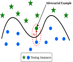
Figure 1: Representation of adversarial attack against machine learning classifier. The objective is to generate a small perturbation $\delta x$ that would result the instance crossing the decision boundary [58].

IV-A Network Architecture

In our experiments, we considered the network architecture provided by [5]. It is a CNN-based network that includes an input layer, convolutional layers, max-pooling layers, and one fully connected layer. The network is characterized by several convolutional layers before the first max pooling layer to enable at a large scale a good reception for each neuron. Additionally, we maintain the maximum spatial information by setting the stride to 1. Accordingly, we deployed the SPRITZ1 and SPRITZ2 networks with different types of datasets (ref. Table  III). It is worth mentioning that we are considering the deep network given its difficulty to compromise compared to the shallow network. Moreover, we rely on such network architecture because it achieves a high accuracy during the training phase. Both networks are configured once as the SN and once as the TN. The architectural details of SPRITZ1 and SPRITZ2 networks are given below.

Table III: General Description of the Considered Networks with their Respective Datasets.

	N-BaIoT	DGA	RIPE
SPRITZ1	$N_{SPRITZ1}^{N-BaIoT}$	$N_{SPRITZ1}^{DGA}$	$N_{SPRITZ1}^{RIPE}$
SPRITZ2	$N_{SPRITZ2}^{N-BaIoT}$	$N_{SPRITZ2}^{DGA}$	$N_{SPRITZ2}^{RIPE}$

IV-A1 SPRITZ1 Network

The configuration of SPRITZ1 is a shallow network that consists of nine convolutional layers, two max-pooling layers, and one fully connected layer. In Figure  2, we illustrate the pipeline of the SPRITZ1 architecture. For all the convolutional layers, we use the kernel size of $3\times 3$ and stride 1. In addition, we applied the max-pooling with the kernel size of $2\times 2$ and stride 2. We note that by halving the number of features maps in the final convolutional layer, we reduce the number of parameters and consider only one fully-connected layer.

Figure 2: Pipeline of the proposed SPRITZ1 architecture (shallow network).

IV-A2 SPRITZ2 Network

In the SPRITZ2 network, we increased the number of convolutional layers to fifteen layers comparing to SPRITZ1. As depicted in Figure 3, the SPRITZ2 network is deeper than SPRITZ1 network. However, we respected the same settings as the SPRITZ1 network. In other words, we used one fully connected layer and two max-pooling layers with the kernel size of $2\times 2$ and stride 1. For all the convolutional layers, we considered the kernel size as $3\times 3$ and stride 1.

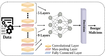
Figure 3: Pipeline of the proposed SPRITZ2 architecture (deep network).

IV-B Experimental Setup

To build our models $N_{SPRITZ1}^{N-BaIoT}$ and $N_{SPRITZ2}^{N-BaIoT}$, for each class, we considered 58000 patches for training, 20000 for validation, and 20000 for testing, per class. The input patch size is set to $64\times 64$ in all the cases. Regarding $N_{SPRITZ1}^{DGA}$ and $N_{SPRITZ2}^{DGA}$, we considered 2000 patches for training and 500 patches for validation and testing, per class. Concerning $N_{SPRITZ1}^{RIPE}$ and $N_{SPRITZ2}^{RIPE}$, we employed 60000 patches for training, 20000 for validation, and 20000 for testing, per class, that we think these number of features enough for a CNN for generalizing. By using small patches, we increase the depth of the network with the same parameters. Consequently, the detection accuracy is increased when aggregating the patch scores. We implemented our CNN, and LSTM networks for training and testing in TensorFlow via the Keras API [59] with Python. We ran our experiments using Intel®Core™ i7-10750H, NVIDIA®GeForce RTX™ 2060 with 6GB GDDR6 GPU, DDR4 16GB*2 (3200MHz), Linux Ubuntu 20.04. We made the simulation Python code publicly available at Github [60]. The number of training epochs is set to 20. We used Adam solver with a learning rate of $10^{-4}$ and a momentum of 0.99. The batch size for training and validation on N-BaIoT, DGA, and RIPE is set to 64, and the test batch size is set to 100.

IV-C Empirical Study

In the experiments, we launched five different adversarial attacks against six classes of networks (ref. Table  III) to highlight the transferability in a large domain. Concretely, for each two different classes of networks, namely the SN (Source Network) and the TN (Target Network), we analyzed the transferability property of adversarial attacks from the SN to the TN. According to Barni et al. [39] and Papernot et al. [12], we split our experiments into three scenarios of transferability. These scenarios are related to the type of mismatch between the SN and the TN (i.e., half mismatch and complete mismatch). We provide in Figure  4 the general scheme of the transferability property in computer networks.

• Cross Training transferability: This scenario is a half mismatch where the SN and TN share the same network architecture. The both networks are trained on two different datasets, namely N-BaIoT and DGA datasets.

• Cross Model transferability: The cross model transferability is also a half mismatch setting. In this scenario, we train the same dataset on two different architectures, namely SPRITZ1 and SPRITZ2.

• Cross Model and Training transferability: This scenario is a complete mismatch where the SN and TN have different architectures and also trained on different datasets.

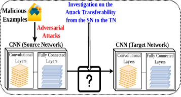
Figure 4: General scheme of the transferability property in computer networks.

The three scenarios resulted in a large set of experiments, and we discuss their outcomes in Section V. Table  IV summarizes the scenarios presented above with their respective SN and TN. To simplify our experiments, we did not consider all possible scenarios. However, the reasonable number of experiments that we conducted is acceptable to conclude the transferability property in computer networks.

Table IV: Scenarios of the Considered Source and Target Networks.

	$N_{1}$	$N_{2}$	$N_{3}$	$N_{4}$	$N_{5}$	$N_{6}$
$N_{1}$		CT	CM	CMT	CT
$N_{2}$	CT			CM
$N_{3}$	CM			CT
$N_{4}$	CMT	CM	CT
$N_{5}$						CM
$N_{6}$						CMT

• $N_{1}$:$N_{SPRITZ1}^{N-BaIoT}$, $N_{2}$:$N_{SPRITZ1}^{DGA}$, $N_{3}$:$N_{SPRITZ2}^{N-BaIoT}$,

• $N_{4}$:$N_{SPRITZ2}^{DGA}$ $N_{5}$:$N_{SPRITZ1}^{RIPE}$, $N_{6}$:$N_{SPRITZ2}^{RIPE}$

V Results and Discussion

In this section, we present the results of our experiments; then, we suggest two defense mechanisms against adversarial transferability. Afterward, we provide a discussion to evaluate the performance of the transferability property in computer networks.

V-A Experimental Results

The test accuracy achieved by SPRITZ1 and SPRITZ2 on the test set N-BaIoT, DGA, and RIPE, detection task is: 99.89% for $N_{SPRITZ1}^{N-BaIoT}$, $N_{SPRITZ2}^{N-BaIoT}$, $N_{SPRITZ2}^{DGA}$, and $N_{SPRITZ2}^{RIPE}$. We achieved the test accuracy 99.50% for $N_{SPRITZ1}^{DGA}$, and 99.20% for $N_{SPRITZ1}^{RIPE}$.
For the I-FGSM attack, we fixed the number of steps to 10, and we considered the normalized strength factor $\varepsilon=0.1$, 0.01, and 0.001, where the average PSNR is above 40 dB. Regarding the JSMA attack, the model parameters $\theta$ are set to 0.1 and 0.01.

The results presented in the following correspond to the average ASR on SN, the average ASR on TN, the average PSNR on 250 samples, the average $L_{1}$ distortion, and the average maximum absolute distortion. During the experiments, we consider the adversarial attack transferability successful if the average ASR threshold is above 50%. We highlight the transferable attacks in bold for each scenario.

Cross Training transferability. We illustrate and report in Table V five case scenarios in the cross training transferability. For the SPRITZ1 network, and given both datasets interchangeably across the SN and the TN. Although the average ASR on the SN is successful (except for the JSMA attack that fails on the SN $N_{SPRITZ1}^{N-BaIoT}$ with the parameter $\theta=0.01$), the transferability property is not satisfied on the TN. More specifically, for all the considered five adversarial attacks, the average ASR on the TN is almost null. Similarly, for the SPRITZ2 network, the adversarial attacks cannot be transferred between the SN and the TN. In particular, we remark that the average ASR on the TN remains almost null. Moreover, the JSMA attack fails on the SN $N_{SPRITZ2}^{N-BaIoT}$ and $N_{SPRITZ2}^{DGA}$ when considering the parameter $\theta=0.01$. In summary, we observe that the adversarial attacks generated are not transferable from the SN to the TN, and in all the cases, the adversary cannot fool the TN. With respect to the training dataset, it is worth mentioning that, for a given computer network, where the SN and TN share the same architecture and are trained on two different datasets, the cross training transferability is asymmetric. In other words, when the datasets are mismatched but the architectures are matched, the I-FGSM, JSMA, LBFGS, PGD, and DeepFool attacks are less transferable in the cross-training transferability. One plausible explanation is that while the attacks only affect a small percentage of the samples, the attacked model tends to overfit more. It’s also worth noting that the transferability of training datasets for a specific task isn’t symmetric. This implies that, mostly in computer networks, the baseline dataset may influence the features learned by the network in some way and to some amount. We considered another dataset, RIPE Atlas, as a TN (SPRITZ1) for a few experiments to better evaluate the transferability performance. When using RIPE Atlas dataset, we have found that attacking on SN is still not enough to deceive TN.

Cross Model transferability. We consider five case scenarios in the cross model transferability, and we describe the experimental results in Table  VI. When training the same datasets on two different networks (SPRITZ1 and SPRITZ2), we can see that the average ASR on the SN is successful (except for the JSMA attack that fails on the SN $N_{SPRITZ1}^{N-BaIoT}$ with the parameter $\theta=0.01$). Moreover, we remark that some adversarial attacks exhibit a transferability between the SN and the TN, such as the JSMA attack, the I-FGSM attack, and the LBFGS attack. For the N-BaIoT datasets, the JSMA attack enables a strong transferability from the SN to the TN when considering the SNs $N_{SPRITZ1}^{N-BaIoT}$ and $N_{SPRITZ2}^{N-BaIoT}$ with the parameter $\theta=0.1$ and $\theta=0.01$ respectively. The experimental results show that the average ASR on the TN is $1$ for $N_{SPRITZ1}^{N-BaIoT}$ as a SN and $0.9960$ for $N_{SPRITZ2}^{N-BaIoT}$ as a SN. Regarding the DGA datasets, the average ASR on the SN is successful (except for the JSMA attack that fails on the SN $N_{SPRITZ2}^{DGA}$ with the parameter $\theta=0.01$), and we achieve the transferability for both the I-FGSM attack and the LBFGS attack. Considering the $N_{SPRITZ2}^{DGA}$ as a SN, the transferability happens for the I-FGSM attack with both parameters $\varepsilon=0.01$ and $\varepsilon=0.001$, and their average ASR on the TN is $1$. Additionally, the LBFGS attack with the default parameter is transferable given the $N_{SPRITZ2}^{DGA}$ as a SN, and the average ASR on the TN is $0.63$. Differently from the previous scenario, the cross model transferability demonstrates five different cases in computer networks where the adversary can perfectly fool the TN. Therefore, the absence of transferability in the JSMA, IFGSM, and LBFGS attacks scenarios in cross-modal transferability is considerably more significant. As a result, we may expect shallow and deep architectures to obtain similar peculiar features in some scenarios, thus enhancing the attack transferability. For additional tests, we used the RIPE dataset in this setting while TN was trained on it. We noticed that non-transferability exists in this scenario as well, when RIPE dataset is employed.

Table V: Experimental Results for Cross Training Transferability on SPRITZ1 and SPRITZ2 Architecture
(N-BaIoT and DGA datasets are used interchangeably in the SN and the TN, while RIPE Atlas dataset is used only in the TN)

. SN TN Accuracy Attack Type PSNR $L_{1}$ dist Max. dist ASR ASR (SN) (TN) $N_{SPRITZ1}^{N-BaIoT}$ $N_{SPRITZ1}^{DGA}$ SN = 98.90% , TN = 100% I-FGSM, $\varepsilon$ = 0.1 18.65 22.07 65.12 1.0000 0.0480 $N_{SPRITZ1}^{N-BaIoT}$ $N_{SPRITZ1}^{DGA}$ SN = 98.90% , TN = 100% I-FGSM, $\varepsilon$ = 0.01 18.93 21.26 62.71 1.0000 0.0000 $N_{SPRITZ1}^{N-BaIoT}$ $N_{SPRITZ1}^{DGA}$ SN = 98.90% , TN = 100% I-FGSM, $\varepsilon$ = 0.001 19.06 20.94 61.76 1.0000 0.0000 $N_{SPRITZ1}^{N-BaIoT}$ $N_{SPRITZ1}^{DGA}$ SN = 98.90% , TN = 100% JSMA, $\theta$ = 0.1 18.49 7.29 178.50 1.0000 0.1100 $N_{SPRITZ1}^{N-BaIoT}$ $N_{SPRITZ1}^{DGA}$ SN = 98.90% , TN = 100% JSMA, $\theta$ = 0.01 – – – FAIL^* – $N_{SPRITZ1}^{N-BaIoT}$ $N_{SPRITZ1}^{DGA}$ SN = 98.90% , TN = 100% LBFGS, default parameter 22.57 9.98 106.35 1.0000 0.0000 $N_{SPRITZ1}^{N-BaIoT}$ $N_{SPRITZ1}^{DGA}$ SN = 98.90% , TN = 100% PGD, default parameter 19.59 19.71 54.00 0.9800 0.0020 $N_{SPRITZ1}^{N-BaIoT}$ $N_{SPRITZ1}^{DGA}$ SN = 98.90% , TN = 100% DeepFool, default parameter 20.90 12.11 142.85 0.9500 0.0400 $N_{SPRITZ1}^{DGA}$ $N_{SPRITZ1}^{N-BaIoT}$ SN = 100% , TN = 98.90% I-FGSM, $\varepsilon$ = 0.1 31.4618 4.81 17.20 1.0000 0.0050 $N_{SPRITZ1}^{DGA}$ $N_{SPRITZ1}^{N-BaIoT}$ SN = 100% , TN = 98.90% I-FGSM, $\varepsilon$ = 0.01 32.51 4.21 15.92 1.0000 0.0000 $N_{SPRITZ1}^{DGA}$ $N_{SPRITZ1}^{N-BaIoT}$ SN = 100% , TN = 98.90% I-FGSM, $\varepsilon$ = 0.001 32.96 4.00 15.03 1.0000 0.0000 $N_{SPRITZ1}^{DGA}$ $N_{SPRITZ1}^{N-BaIoT}$ SN = 100% , TN = 98.90% JSMA, $\theta$ = 0.1 31.23 1.47 62.50 1.0000 0.2000 $N_{SPRITZ1}^{DGA}$ $N_{SPRITZ1}^{N-BaIoT}$ SN = 100% , TN = 98.90% JSMA, $\theta$ = 0.01 35.95 1.077 17.85 1.0000 0.0010 $N_{SPRITZ1}^{DGA}$ $N_{SPRITZ1}^{N-BaIoT}$ SN = 100% , TN = 98.90% LBFGS, default parameter 37.19 1.41 23.38 1.0000 0.0000 $N_{SPRITZ1}^{DGA}$ $N_{SPRITZ1}^{N-BaIoT}$ SN = 100% , TN = 98.90% PGD, default parameter 33.75 3.58 13.93 1.0000 0.0000 $N_{SPRITZ1}^{DGA}$ $N_{SPRITZ1}^{N-BaIoT}$ SN = 100% , TN = 98.90% DeepFool, default parameter 36.98 2.20 38.08 1.0000 0.0300 $N_{SPRITZ2}^{N-BaIoT}$ $N_{SPRITZ2}^{DGA}$ SN = 98.90% , TN = 100% I-FGSM, $\varepsilon$ = 0.1 17.98 22.67 58.06 1.0000 0.0360 $N_{SPRITZ2}^{N-BaIoT}$ $N_{SPRITZ2}^{DGA}$ SN = 98.90% , TN = 100% I-FGSM, $\varepsilon$ = 0.01 18.64 20.96 53.47 1.0000 0.0000 $N_{SPRITZ2}^{N-BaIoT}$ $N_{SPRITZ2}^{DGA}$ SN = 98.90% , TN = 100% I-FGSM, $\varepsilon$ = 0.001 18.71 20.82 53.16 1.0000 0.0000 $N_{SPRITZ2}^{N-BaIoT}$ $N_{SPRITZ2}^{DGA}$ SN = 98.90% , TN = 100% JSMA, $\theta$ = 0.1 22.23 2.91 178.08 1.0000 0.0061 $N_{SPRITZ2}^{N-BaIoT}$ $N_{SPRITZ2}^{DGA}$ SN = 98.90% , TN = 100% JSMA, $\theta$ = 0.01 – – – FAIL^* – $N_{SPRITZ2}^{N-BaIoT}$ $N_{SPRITZ2}^{DGA}$ SN = 98.90% , TN = 100% LBFGS, default parameter 24.62 4.67 194.25 1.0000 0.0000 $N_{SPRITZ2}^{N-BaIoT}$ $N_{SPRITZ2}^{DGA}$ SN = 98.90% , TN = 100% PGD, default parameter 18.75 20.66 53.07 0.9916 0.1812 $N_{SPRITZ2}^{N-BaIoT}$ $N_{SPRITZ2}^{DGA}$ SN = 98.90% , TN = 100% DeepFool, default parameter 23.86 4.59 177.38 1.0000 0.0000 $N_{SPRITZ2}^{DGA}$ $N_{SPRITZ2}^{N-BaIoT}$ SN = 100% , TN = 98.90% I-FGSM, $\varepsilon$ = 0.1 28.48 6.03 25.15 0.9800 0.0150 $N_{SPRITZ2}^{DGA}$ $N_{SPRITZ2}^{N-BaIoT}$ SN = 100% , TN = 98.90% I-FGSM, $\varepsilon$ = 0.01 28.61 5.99 23.34 1.0000 0.0000 $N_{SPRITZ2}^{DGA}$ $N_{SPRITZ2}^{N-BaIoT}$ SN = 100% , TN = 98.90% I-FGSM, $\varepsilon$ = 0.001 28.92 5.76 22.64 1.0000 0.0000 $N_{SPRITZ2}^{DGA}$ $N_{SPRITZ2}^{N-BaIoT}$ SN = 100% , TN = 98.90% JSMA, $\theta$ = 0.1 31.17 1.28 56.56 1.0000 0.1000 $N_{SPRITZ2}^{DGA}$ $N_{SPRITZ2}^{N-BaIoT}$ SN = 100% , TN = 98.90% JSMA, $\theta$ = 0.01 – – – FAIL^* – $N_{SPRITZ2}^{DGA}$ $N_{SPRITZ2}^{N-BaIoT}$ SN = 100% , TN = 98.90% LBFGS, default parameter 34.22 1.40 33.93 1.0000 0.0000 $N_{SPRITZ2}^{DGA}$ $N_{SPRITZ2}^{N-BaIoT}$ SN = 100% , TN = 98.90% PGD, default parameter 29.24 5.49 22.24 1.0000 0.0000 $N_{SPRITZ2}^{DGA}$ $N_{SPRITZ2}^{N-BaIoT}$ SN = 100% , TN = 98.90% DeepFool, default parameter 31.02 2.25 53.42 0.9812 0.1200 $N_{SPRITZ1}^{N-BaIoT}$ $N_{SPRITZ1}^{RIPE}$ SN = 98.90% , TN = 99.20% I-FGSM, $\varepsilon$ = 0.1 18.65 22.07 65.12 1.0000 0.0200 $N_{SPRITZ1}^{N-BaIoT}$ $N_{SPRITZ1}^{RIPE}$ SN = 98.90% , TN = 99.20% JSMA, $\theta$ = 0.1 18.49 7.29 178.50 1.0000 0.0000 $N_{SPRITZ1}^{N-BaIoT}$ $N_{SPRITZ1}^{RIPE}$ SN = 98.90% , TN = 99.20% LBFGS, default parameter 22.57 9.98 106.35 1.0000 0.0010 $N_{SPRITZ1}^{N-BaIoT}$ $N_{SPRITZ1}^{RIPE}$ SN = 98.90% , TN = 99.20% PGD, default parameter 19.59 19.71 54.00 0.9800 0.0000 $N_{SPRITZ1}^{DGA}$ $N_{SPRITZ1}^{RIPE}$ SN = 98.90% , TN = 99.20% DeepFool, default parameter 36.98 2.20 38.08 1.0000 0.0000
FAIL^*: In this case, the attack on the source network fails and we cannot transfer it to the target network. Therefore, the numerical values of the average PSNR, the average $L_{1}$ dist, and the average maximum distortion are not possible.

Table VI: Experimental Results for Cross Model Transferability on N-BaIoT, DGA, and RIPE Atlas datasets
(SPRITZ1 and SPRITZ2 are used interchangeably in the SN and the TN).

SN	TN	Accuracy	Attack Type	PSNR	$L_{1}$ dist	Max. dist	ASR	ASR
							(SN)	(TN)
$N_{SPRITZ1}^{N-BaIoT}$	$N_{SPRITZ2}^{N-BaIoT}$	SN = 98.90% , TN = 98.80%	I-FGSM, $\varepsilon$ = 0.1	18.65	22.07	64.78	1.0000	0.0030
$N_{SPRITZ1}^{N-BaIoT}$	$N_{SPRITZ2}^{N-BaIoT}$	SN = 98.90% , TN = 98.80%	I-FGSM, $\varepsilon$ = 0.01	18.93	21.26	62.71	1.0000	0.0000
$N_{SPRITZ1}^{N-BaIoT}$	$N_{SPRITZ2}^{N-BaIoT}$	SN = 98.90% , TN = 98.80%	I-FGSM, $\varepsilon$ = 0.001	19.04	20.94	61.76	1.0000	0.0000
$N_{SPRITZ1}^{N-BaIoT}$	$N_{SPRITZ2}^{N-BaIoT}$	SN = 98.90% , TN = 98.80%	JSMA, $\theta$ = 0.1	18.49	7.29	170.50	1.0000	1.0000
$N_{SPRITZ1}^{N-BaIoT}$	$N_{SPRITZ2}^{N-BaIoT}$	SN = 98.90% , TN = 98.80%	JSMA, $\theta$ = 0.01	–	–	–	FAIL*	–
$N_{SPRITZ1}^{N-BaIoT}$	$N_{SPRITZ2}^{N-BaIoT}$	SN = 98.90% , TN = 98.80%	LBFGS, default parameter	22.57	9.98	106.42	0.9960	0.0040
$N_{SPRITZ1}^{N-BaIoT}$	$N_{SPRITZ2}^{N-BaIoT}$	SN = 98.90% , TN = 98.80%	PGD, default parameter	19.59	19.71	54.00	1.0000	0.0104
$N_{SPRITZ1}^{N-BaIoT}$	$N_{SPRITZ2}^{N-BaIoT}$	SN = 98.90% , TN = 98.80%	Deepfool, default parameter	20.86	12.15	143.31	0.9190	0.1336
$N_{SPRITZ2}^{N-BaIoT}$	$N_{SPRITZ1}^{N-BaIoT}$	SN = 98.90% , TN = 98.80%	I-FGSM, $\varepsilon$ = 0.1	17.98	22.67	58.06	0.9913	0.0200
$N_{SPRITZ2}^{N-BaIoT}$	$N_{SPRITZ1}^{N-BaIoT}$	SN = 98.90% , TN = 98.80%	I-FGSM, $\varepsilon$ = 0.01	18.65	20.96	53.47	1.0000	0.0000
$N_{SPRITZ2}^{N-BaIoT}$	$N_{SPRITZ1}^{N-BaIoT}$	SN = 98.90% , TN = 98.80%	I-FGSM, $\varepsilon$ = 0.001	18.71	20.82	53.16	1.0000	0.0000
$N_{SPRITZ2}^{N-BaIoT}$	$N_{SPRITZ1}^{N-BaIoT}$	SN = 98.90% , TN = 98.80%	JSMA, $\theta$ = 0.1	22.23	2.91	178.08	1.0000	0.0000
$N_{SPRITZ2}^{N-BaIoT}$	$N_{SPRITZ1}^{N-BaIoT}$	SN = 98.90% , TN = 98.80%	JSMA, $\theta$ = 0.01	40.93	0.30	17.84	1.0000	0.9960
$N_{SPRITZ2}^{N-BaIoT}$	$N_{SPRITZ1}^{N-BaIoT}$	SN = 98.90% , TN = 98.80%	LBFGS, default parameter	24.62	4.67	114.36	1.0000	0.0000
$N_{SPRITZ2}^{N-BaIoT}$	$N_{SPRITZ1}^{N-BaIoT}$	SN = 98.90% , TN = 98.80%	PGD, default parameter	18.75	20.66	53.07	1.0000	0.0000
$N_{SPRITZ2}^{N-BaIoT}$	$N_{SPRITZ1}^{N-BaIoT}$	SN = 98.90% , TN = 98.80%	DeepFool, default parameter	23.86	4.59	177.38	1.0000	0.0000
$N_{SPRITZ1}^{DGA}$	$N_{SPRITZ2}^{DGA}$	SN = 99.60% , TN = 99.60%	I-FGSM, $\varepsilon$ = 0.1	31.46	4.81	17.20	1.0000	0.0100
$N_{SPRITZ1}^{DGA}$	$N_{SPRITZ2}^{DGA}$	SN = 99.60% , TN = 99.60%	I-FGSM, $\varepsilon$ = 0.01	32.51	4.21	15.92	1.0000	0.0000
$N_{SPRITZ1}^{DGA}$	$N_{SPRITZ2}^{DGA}$	SN = 99.60% , TN = 99.60%	I-FGSM, $\varepsilon$ = 0.001	32.96	4.00	15.03	1.0000	0.0000
$N_{SPRITZ1}^{DGA}$	$N_{SPRITZ2}^{DGA}$	SN = 99.60% , TN = 99.60%	JSMA, $\theta$ = 0.1	31.23	1.47	62.50	1.0000	0.5020
$N_{SPRITZ1}^{DGA}$	$N_{SPRITZ2}^{DGA}$	SN = 99.60% , TN = 99.60%	JSMA, $\theta$ = 0.01	35.95	1.07	17.85	1.0000	0.0900
$N_{SPRITZ1}^{DGA}$	$N_{SPRITZ2}^{DGA}$	SN = 99.60% , TN = 99.60%	LBFGS, default parameter	37.19	1.47	23.20	0.9930	0.0400
$N_{SPRITZ1}^{DGA}$	$N_{SPRITZ2}^{DGA}$	SN = 99.60% , TN = 99.60%	PGD, default parameter	33.75	3.58	13.93	1.0000	0.0000
$N_{SPRITZ1}^{DGA}$	$N_{SPRITZ2}^{DGA}$	SN = 99.60% , TN = 99.60%	DeepFool, default parameter	34.11	2.20	38.21	1.0000	0.0000
$N_{SPRITZ2}^{DGA}$	$N_{SPRITZ1}^{DGA}$	SN = 99.60% , TN = 99.60%	I-FGSM, $\varepsilon$ = 0.1	28.48	6.04	24.15	1.0000	0.4100
$N_{SPRITZ2}^{DGA}$	$N_{SPRITZ1}^{DGA}$	SN = 99.60% , TN = 99.60%	I-FGSM, $\varepsilon$ = 0.01	28.62	5.99	23.25	1.0000	1.0000
$N_{SPRITZ2}^{DGA}$	$N_{SPRITZ1}^{DGA}$	SN = 99.60% , TN = 99.60%	I-FGSM, $\varepsilon$ = 0.001	28.92	5.76	22.64	1.0000	1.0000
$N_{SPRITZ2}^{DGA}$	$N_{SPRITZ1}^{DGA}$	SN = 99.60% , TN = 99.60%	JSMA, $\theta$ = 0.1	31.17	1.28	56.56	1.0000	0.0000
$N_{SPRITZ2}^{DGA}$	$N_{SPRITZ1}^{DGA}$	SN = 99.60% , TN = 99.60%	JSMA, $\theta$ = 0.01	–	–	–	FAIL*	–
$N_{SPRITZ2}^{DGA}$	$N_{SPRITZ1}^{DGA}$	SN = 99.60% , TN = 99.60%	LBFGS, default parameter	34.22	1.48	33.92	0.9930	0.6300
$N_{SPRITZ2}^{DGA}$	$N_{SPRITZ1}^{DGA}$	SN = 99.60% , TN = 99.60%	PGD, default parameter	29.24	5.49	22.24	1.0000	0.3200
$N_{SPRITZ2}^{DGA}$	$N_{SPRITZ1}^{DGA}$	SN = 99.60% , TN = 99.60%	DeepFool, default parameter	31.02	2.25	53.42	1.0000	0.2329
$N_{SPRITZ1}^{RIPE}$	$N_{SPRITZ2}^{RIPE}$	SN = 98.90% , TN = 99.80%	I-FGSM, $\varepsilon$ = 0.1	18.65	22.07	64.78	1.0000	0.0000
$N_{SPRITZ1}^{RIPE}$	$N_{SPRITZ2}^{RIPE}$	SN = 98.90% , TN = 99.80%	JSMA, $\theta$ = 0.1	18.49	7.29	170.50	1.0000	0.0140
$N_{SPRITZ1}^{RIPE}$	$N_{SPRITZ2}^{RIPE}$	SN = 98.90% , TN = 99.80%	LBFGS, default parameter	22.57	9.98	106.42	0.9960	0.0100
$N_{SPRITZ1}^{RIPE}$	$N_{SPRITZ2}^{RIPE}$	SN = 99.60% , TN = 99.80%	PGD, default parameter	33.75	3.58	13.93	1.0000	0.0020
$N_{SPRITZ1}^{RIPE}$	$N_{SPRITZ2}^{RIPE}$	SN = 99.60% , TN = 99.80%	DeepFool, default parameter	34.11	2.20	38.21	1.0000	0.0000

FAIL^*: In this case, the attack on the source network fails and we cannot transfer it to the target network. Therefore, the numerical values of the average PSNR, the average $L_{1}$ dist, and the average maximum distortion are not possible.

Table VII: Experimental results for Cross Model and Training Transferability (The architectures and datasets
are used interchangeably in the SN an the TN, except for RIPE Atlas dataset which is used only in the TN)

SN	TN	Accuracy	Attack Type	PSNR	$L_{1}$ dist	Max. dist	ASR	ASR
							(SN)	(TN)
$N_{SPRITZ1}^{N-BaIoT}$	$N_{SPRITZ2}^{DGA}$	SN = 98.80% , TN = 100%	I-FGSM, $\varepsilon$ = 0.1	18.65	22.07	64.78	1.0000	0.0030
$N_{SPRITZ1}^{N-BaIoT}$	$N_{SPRITZ2}^{DGA}$	SN = 98.80% , TN = 100%	I-FGSM, $\varepsilon$ = 0.01	18.93	21.26	62.71	1.0000	0.0000
$N_{SPRITZ1}^{N-BaIoT}$	$N_{SPRITZ2}^{DGA}$	SN = 98.80% , TN = 100%	I-FGSM, $\varepsilon$ = 0.001	19.06	20.93	61.72	1.0000	0.0000
$N_{SPRITZ1}^{N-BaIoT}$	$N_{SPRITZ2}^{DGA}$	SN = 98.80% , TN = 100%	JSMA, $\theta$ = 0.1	18.49	7.29	178.50	1.0000	0.0000
$N_{SPRITZ1}^{N-BaIoT}$	$N_{SPRITZ2}^{DGA}$	SN = 98.80% , TN = 100%	JSMA, $\theta$ = 0.01	–	–	–	FAIL*	–
$N_{SPRITZ1}^{N-BaIoT}$	$N_{SPRITZ2}^{DGA}$	SN = 98.80% , TN = 100%	LBFGS, default parameter	22.57	10.46	110.67	0.9910	0.0000
$N_{SPRITZ1}^{N-BaIoT}$	$N_{SPRITZ2}^{DGA}$	SN = 98.80% , TN = 100%	PGD, default parameter	19.59	19.71	54.00	1.0000	0.0000
$N_{SPRITZ1}^{N-BaIoT}$	$N_{SPRITZ2}^{DGA}$	SN = 98.80% , TN = 100%	DeepFool, default parameter	20.87	12.14	143.19	0.9676	0.0324
$N_{SPRITZ2}^{DGA}$	$N_{SPRITZ1}^{N-BaIoT}$	SN = 99.60% , TN = 99.60%	I-FGSM, $\varepsilon$ = 0.1	28.49	6.03	24.15	1.0000	0.0400
$N_{SPRITZ2}^{DGA}$	$N_{SPRITZ1}^{N-BaIoT}$	SN = 99.60% , TN = 99.60%	I-FGSM, $\varepsilon$ = 0.01	28.62	5.99	23.25	1.0000	0.0000
$N_{SPRITZ2}^{DGA}$	$N_{SPRITZ1}^{N-BaIoT}$	SN = 99.60% , TN = 99.60%	I-FGSM, $\varepsilon$ = 0.001	28.92	5.76	22.64	1.0000	0.0000
$N_{SPRITZ2}^{DGA}$	$N_{SPRITZ1}^{N-BaIoT}$	SN = 99.60% , TN = 99.60%	JSMA, $\theta$ = 0.1	31.17	1.28	56.56	1.0000	0.0000
$N_{SPRITZ2}^{DGA}$	$N_{SPRITZ1}^{N-BaIoT}$	SN = 99.60% , TN = 99.60%	JSMA, $\theta$ = 0.01	–	–	–	FAIL*	–
$N_{SPRITZ2}^{DGA}$	$N_{SPRITZ1}^{N-BaIoT}$	SN = 99.60% , TN = 99.60%	LBFGS, default parameter	34.22	1.40	33.93	0.9860	0.0040
$N_{SPRITZ2}^{DGA}$	$N_{SPRITZ1}^{N-BaIoT}$	SN = 99.60% , TN = 99.60%	PGD, default parameter	29.24	5.99	22.24	1.0000	0.0000
$N_{SPRITZ2}^{DGA}$	$N_{SPRITZ1}^{N-BaIoT}$	SN = 99.60% , TN = 99.60%	DeepFool, default parameter	31.02	2.59	53.42	1.0000	0.0104
$N_{SPRITZ1}^{N-BaIoT}$	$N_{SPRITZ2}^{RIPE}$	SN = 98.80% , TN = 99.80%	I-FGSM, $\varepsilon$ = 0.1	18.65	22.07	64.78	1.0000	0.0000
$N_{SPRITZ1}^{N-BaIoT}$	$N_{SPRITZ2}^{RIPE}$	SN = 98.80% , TN = 99.80%	JSMA, $\theta$ = 0.1	18.49	7.29	178.50	1.0000	0.0010
$N_{SPRITZ1}^{N-BaIoT}$	$N_{SPRITZ2}^{RIPE}$	SN = 98.80% , TN = 99.80%	LBFGS, default parameter	22.57	10.46	110.67	0.9910	0.0000
$N_{SPRITZ1}^{N-BaIoT}$	$N_{SPRITZ2}^{RIPE}$	SN = 98.80% , TN = 99.80%	PGD, default parameter	19.59	19.71	54.00	1.0000	0.0000
$N_{SPRITZ1}^{N-BaIoT}$	$N_{SPRITZ2}^{RIPE}$	SN = 98.80% , TN = 99.80%	DeepFool, default parameter	20.87	12.14	143.19	0.9676	0.0200

FAIL^*: In this case, the attack on the source network fails and we cannot transfer it to the target network. Therefore, the numerical values of the average PSNR, the average $L_{1}$ dist, and the average maximum distortion are not possible.

Cross Model and Training transferability. We consider three case scenarios, and present in Table  VII our evaluation on two different networks (SPRITZ1 and SPRITZ2) that are trained on three different datasets (N-BaIoT, DGA, and RIPE Atlas). As it can be seen, the average ASR on the SN is successful (except for the JSMA attack that fails on the SN $N_{SPRITZ1}^{N-BaIoT}$ with the parameter $\theta=0.01$, and the SN $N_{SPRITZ2}^{DGA}$ with the parameters $\theta=0.01$). We notice that none of the five adversarial attacks performed in our experiments are transferable from the SN to the TN, and the average ASR on the TN is almost null. Therefore, the feasibility of the cross model and training transferability in computer networks is unlikely hard to happen. Table VII shows that, in this scenario, the attack success rate decreases, as we have a full mismatch in networks and datasets. For additional experiments, we used the RIPE as a mismatch dataset for TN. In a complete mismatch setting, we conclude that SN and TN are non-transferable. Figure 5 shows a visual representation of adversarial attacks that transfer from SN to TN.

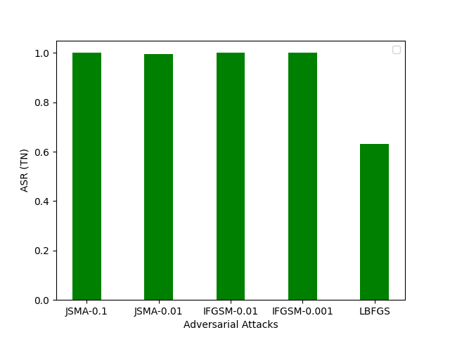
Figure 5: Summary of transferability cases where adversarial attacks transfer between SN to TN.

V-B Anti-Exploratory Evasion Defense mechanisms

The outcomes of our study reveal that the adversarial samples are often non-transferable, contrary to what we observe in standard classification tasks, such as multimedia forensics and similar applications. This finding is important because we can leverage the limitation of transferability to hinder the attack. For instance, an LK scenario could be imposed somehow, as with standard ML techniques, to prevent adversarial examples. However, we identified various adversarial attacks in different scenarios that enable the transferability property, meaning that the adversarial attacks can entirely mislead the TN. In this case, we suggest two current defense mechanisms that prevent adversarial transferability. The first strategy consists of fine-tuning the classifier using the Most Powerful Attacks (MPAs) whenever the transferability happens for a given adversarial attack [16]. Consequently, we improve the security of the TN against different adversarial attacks only for the attacks that transfer between the SN and TN (refer to Table VI). We apply the fine-tuning technique on the TN, and we report our results in Table VIII. Another strategy to prevent adversarial transferability relies on using the LSTM architecture as the TN rather than the CNN, namely as mismatch architecture. Therefore, the TN is different from the classification structure of the original CNN. In this strategy, the attacker has less attack information than the previous system with no knowledge of the TN architecture. We verify this approach in a Cross-Model setting by considering two adversarial attacks enabling the transferability: the JSMA attack with a parameter $\theta$ = 0.01 and the LBFGS attack with a default parameter. Then, we changed the TN architecture from CNN to LSTM. In this scenario, the ASR on the TN significantly decreased in the JSMA attack from 0.9960 to 0.2360 and in the LBFGS attack from 0.6300 to 0.0010. The outcomes of this technique demonstrate that changing the architecture (i.e., SN (CNN) and TN (LSTM)) can significantly prevent adversarial attacks transferability and hence improve the security of the TN. Consequently, the architectural mismatch between the original CNN and the new detector TN is sufficient to prohibit transferability, which may be considered as a shielding strategy.

Table VIII: Test Accuracy Values TN with an MPA fine-tunning.

TN	Fine-Tune	Parameter	I-FGSM, $\varepsilon$ = 0.01	IFGSM, $\varepsilon$ = 0.001	LBFGS, Default	JSMA, $\theta$ = 0.01
$N_{SPRITZ1}^{N-BaIoT}$	JSMA	$\theta$ = 0.01	0.0000	0.0100	0.2010	—
$N_{SPRITZ1}^{DGA}$	I-FGSM	$\varepsilon$ = 0.01	—	0.0000	0.0010	0.0000
$N_{SPRITZ1}^{DGA}$	I-FGSM	$\varepsilon$ = 0.001	0.0000	—	0.0010	0.0000
$N_{SPRITZ1}^{DGA}$	LBFGS	Default	0.0200	0.0010	—	0.0000

V-C Discussion

Table IX: Execution running attack time on SN in seconds.

SN	Attack Type	Dataset1	Dataset2	Dataset3	{Exe. seconds (Dataset1)	Exe. seconds (Dataset2)	Exe. seconds (Dataset3)
SPRITZ1	I-FGSM, $\varepsilon$ = 0.1	N-BaIoT	DGA	RIPE	127.2	127.8	130.8
SPRITZ1	I-FGSM, $\varepsilon$ = 0.01	N-BaIoT	DGA	RIPE	1229.4	1294.2	—
SPRITZ1	I-FGSM, $\varepsilon$ = 0.001	N-BaIoT	DGA	RIPE	12238.8	12766.2	—
SPRITZ1	JSMA, $\theta$ = 0.1	N-BaIoT	DGA	RIPE	1824.6	625.2	1840.2
SPRITZ1	LBFGS, default parameter	N-BaIoT	DGA	RIPE	2923.8	1555.2	2455.2
SPRITZ1	PGD, default parameter	N-BaIoT	DGA	RIPE	1015.2	970.2	976.2
SPRITZ1	DeepFool, default parameter	N-BaIoT	DGA	RIPE	29.4	13.8	22.8
SPRITZ2	I-FGSM, $\varepsilon$ = 0.1	N-BaIoT	DGA	RIPE	265.2	269.4	—
SPRITZ2	I-FGSM, $\varepsilon$ = 0.01	N-BaIoT	DGA	RIPE	2636.4	2698.8	—
SPRITZ2	I-FGSM, $\varepsilon$ = 0.001	N-BaIoT	DGA	RIPE	26306.16	26818.14	—
SPRITZ2	JSMA, $\theta$ = 0.1	N-BaIoT	DGA	RIPE	1954.8	1231.8	—
SPRITZ2	LBFGS, default parameter	N-BaIoT	DGA	RIPE	4723.8	3115.8	—
SPRITZ2	PGD, default parameter	N-BaIoT	DGA	RIPE	2715	2016	—
SPRITZ2	DeepFool, default parameter	N-BaIoT	DGA	RIPE	18.6	22.2	—

Combining all the experimental results, we demonstrate that among five different adversarial attacks, three of them are transferable from the SN to the TN, which are: the JSMA attack, the I-FGSM attack, and the LBFGS attack. Therefore, given a CNN-based model in computer network, specific cases of generated adversarial examples can perfectly fool another network model even with different architectures. In particular, we found that both models in the SN and TN enable the same misclassification; hence, the transferability property. To that end, the adversary can leverage a surrogate model with different architectures and classes of algorithms to approximate the adversarial example for the TN. We note that in the cross model transferability, the features learned by the network might influence somehow to some degree by the underlying dataset, and this aspect requires additional research.

Moreover, we performed multiple adversarial attacks on the SN for 250 manipulated examples to evaluate their computational cost. On the other hand, after detecting adversarial attacks on SN, we remark that the processing testing time for TN is relatively fast. In Table IX, we report our results on the execution running attack time on SN in seconds. This study, as we expected, will also address the issue of usability in botnet attacks. To elaborate more, the authors in [61] suggested a solution for botnet attack detection in the IoT environment using CNN. As a result, most ML and DL methods are subject to various adversarial attacks if we have a classification algorithm for botnet detection. Additionally, the experts in the research area demonstrate that an attack in the SN might not be enough to deceive the TN, based on our studies and other research in computer networks.

VI Conclusions and Future Work

In this paper, we thoroughly dissected the transferability of adversarial examples in computer networks. We investigated three transferability scenarios: the cross training, the cross model, and the cross model and training. Considering three well-known datasets (N-BaIoT, DGA, and RIPE Atlas), we found that the transferability happens in specific cases where the adversary can perfectly transfer the examples from the SN to the TN. Although in other cases, such as the Cross Model and Training transferability, it is difficult to transfer the adversarial examples from the SN to the TN. The adversary still leverages the existing cases where the transferability happens. Due to the black-box nature of deep neural networks, our understanding is very narrow regarding the decisions enabling the transferability between the CNN-based models. This knowledge gap is a critical issue, especially for security-oriented applications in computer networks. Therefore, additional research is required to understand what are the main factors responsible for the transferability property.

According to our experiments, the JSMA and I-FGSM attacks are more transferable than other adversarial attacks, particularly in the cross model transferability. One probable rationale is that when JSMA and I-FGSM attacks alter particular features (those to which the network is more vulnerable), it is likely to overfit the attacked model. It is also worth noting that the transferability is not symmetric in terms of the training datasets for a particular task. These results indicate that the underlying dataset may influence the network’s learned features in some way and to some extent in computer network applications. Thus, we need to investigate this area in future work to understand why computer networks are less vulnerable to attack transferability. Our future work will focus on improving the power of adversarial attacks to increase their transferability. However, this is not a straightforward process, considering the complexity of the decision boundary learned by CNNs or even other deep neural networks.

Ehsan Nowroozi received his doctorate at the University of Siena in Italy. He is a postdoctoral researcher at Sabanci University’s Faculty of Engineering and Natural Sciences (FENS), Istanbul, Turkey’s Center of Excellence in Data Analytics (VERIM). In the years 2020 and 2021, he was a Postdoctoral Researcher at Siena University and Padova University in Italy. His principal research interests are in the fields of security and privacy, with a focus on the use of image processing algorithms in multimedia authentication (multimedia forensics), network and internet security, and other areas. His professional service and activity as a reviewer for IEEE TNSM, IEEE TIFS, IEEE TNNLS, Elsevier journal Digital, EURASIP Journal on Information Security.

Yassine Mekdad received a Msc Degree in Cryptography and Information Security from Mohammed V University of Rabat, Morocco. He works with the Computer Networks and Systems Laboratory at Moulay Ismail University of Meknes, Morocco. He holds a guest researcher position with the SPRITZ research group at University of Padua, Italy. He is currently working as a Research Scholar at the Cyber-Physical Systems Security Lab (CSL) at Florida International University, Miami, FL, USA. His research interest principally cover security and privacy problems in the Internet of Things (IoT), Industrial Internet-of-Things (IIoT), and Cyber-physical systems (CPS).

Mohammad Hajian Berenjestanaki is currently a research assistant at the SPRITZ security and privacy research group, University of Padua, Italy. He completed his bachelor’s degree in Electrical Engineering, Electronics at University of Mazandaran, Iran. He did his Master’s degree in Electrical Engineering, Communications, Cryptography in 2016 at the University of Tehran. His areas of interests include Networks Security and Cryptography, Deep Learning and Machine learning, Block-chain and Distributed Ledger Technology. He conducts his new researches in applied machine learning in Cybersecurity.

Mauro Conti received the Ph.D. degree from the Sapienza University of Rome, Italy. He is a Full Professor with the University of Padua, Italy, and an Affiliate Professor with TU Delft and University of Washington, Seattle. He was a Postdoctoral Researcher with Vrije niversiteit Amsterdam, The Netherlands. In 2011, he joined as an Assistant Professor with the University of Padua, where he became an Associate Professor in 2015, and a Full Professor in 2018. He has been a Visiting Researcher with GMU, UCLA, UCI, TU Darmstadt, UF, and FIU. His research is also funded by companies, including Cisco, Intel, and Huawei. He has been awarded with a Marie Curie Fellowship by the European Commission, and with a Fellowship by the German DAAD.

Abdeslam El Fergougui received the PhD degree in Computer Science from Mohammed V University in Rabat - Morocco. He is currently a professor in the department of Computer science, Faculty of sciences Meknes, Moulay Ismail University. His current research interests include Network, Sensor Network, cryptography, security. Furthermore, he assured several advanced training workshops in its field of action. He also assured several training courses in several Moroccan and international universities. He has managed several national and international projects. He is an active member of AUF (University Agency of Francophonie) where he provides training at the international level. He is a member of the reading committee of several journals and conferences in his field.

References

- [1] S. Dong, P. Wang, and K. Abbas, “A survey on deep learning and its applications,” Computer Science Review, vol. 40, p. 100379, 2021.
- [2] K. Sirinukunwattana, S. E. A. Raza, Y.-W. Tsang, D. R. Snead, I. A. Cree, and N. M. Rajpoot, “Locality sensitive deep learning for detection and classification of nuclei in routine colon cancer histology images,” IEEE transactions on medical imaging, vol. 35, no. 5, pp. 1196–1206, 2016.
- [3] R. Vinayakumar, K. P. Soman, and P. Poornachandran, “Applying convolutional neural network for network intrusion detection,” in 2017 International Conference on Advances in Computing, Communications and Informatics (ICACCI), 2017, pp. 1222–1228.
- [4] A. Anand, S. Rani, D. Anand, H. M. Aljahdali, and D. Kerr, “An efficient cnn-based deep learning model to detect malware attacks (cnn-dma) in 5g-iot healthcare applications,” Sensors, vol. 21, no. 19, 2021.
- [5] M. Barni, A. Costanzo, E. Nowroozi, and B. Tondi, “Cnn-based detection of generic contrast adjustment with jpeg post-processing,” in 25th IEEE International Conference on Image Processing (ICIP). IEEE, 2018, pp. 3803–3807.
- [6] D. Zügner, O. Borchert, A. Akbarnejad, and S. Günnemann, “Adversarial attacks on graph neural networks: Perturbations and their patterns,” ACM Transactions on Knowledge Discovery from Data (TKDD), vol. 14, no. 5, pp. 1–31, 2020.
- [7] E. Nowroozi, A. Dehghantanha, R. M. Parizi, and K.-K. R. Choo, “A survey of machine learning techniques in adversarial image forensics,” Computers & Security, p. 102092, 2020.
- [8] K. Grosse, N. Papernot, P. Manoharan, M. Backes, and P. McDaniel, “Adversarial examples for malware detection,” in European symposium on research in computer security. Springer, 2017, pp. 62–79.
- [9] N. Papernot, P. McDaniel, S. Jha, M. Fredrikson, Z. B. Celik, and A. Swami, “The limitations of deep learning in adversarial settings,” in IEEE European symposium on security and privacy (EuroS&P). IEEE, 2016, pp. 372–387.
- [10] J. Zhang and C. Li, “Adversarial examples: Opportunities and challenges,” IEEE transactions on neural networks and learning systems, vol. 31, no. 7, pp. 2578–2593, 2019.
- [11] C. Szegedy, W. Zaremba, I. Sutskever, J. Bruna, D. Erhan, I. Goodfellow, and R. Fergus, “Intriguing properties of neural networks,” arXiv preprint arXiv:1312.6199, 2013.
- [12] N. Papernot, P. McDaniel, and I. Goodfellow, “Transferability in machine learning: from phenomena to black-box attacks using adversarial samples,” arXiv preprint arXiv:1605.07277, 2016.
- [13] L. Wu, Z. Zhu, C. Tai et al., “Understanding and enhancing the transferability of adversarial examples,” arXiv preprint arXiv:1802.09707, 2018.
- [14] F. Marra, D. Gragnaniello, and L. Verdoliva, “On the vulnerability of deep learning to adversarial attacks for camera model identification,” Signal Processing: Image Communication, vol. 65, pp. 240–248, 2018.
- [15] F. Tramèr, N. Papernot, I. Goodfellow, D. Boneh, and P. McDaniel, “The space of transferable adversarial examples,” arXiv preprint arXiv:1704.03453, 2017.
- [16] M. Barni, E. Nowroozi, and B. Tondi, “Higher-order, adversary-aware, double jpeg-detection via selected training on attacked samples,” in 2017 25th European Signal Processing Conference (EUSIPCO), 2017, pp. 281–285.
- [17] “UCI Machine Learning Repository: detection_of_IoT_botnet_attacks_N_BaIoT Data Set.” [Online]. Available: https://archive.ics.uci.edu/ml/datasets/detection_of_IoT_botnet_attacks_N_BaIoT
- [18] S. Upadhyay and A. Ghorbani, “Feature extraction approach to unearth domain generating algorithms (dgas),” in IEEE International Conference on Dependable, Autonomic and Secure Computing, 2020, pp. 399–405.
- [19] R. N. Staff, “Ripe atlas: A global internet measurement network,” Internet Protocol Journal, vol. 18, no. 3, 2015.
- [20] H. Tahaei, F. Afifi, A. Asemi, F. Zaki, and N. B. Anuar, “The rise of traffic classification in iot networks: A survey,” Journal of Network and Computer Applications, vol. 154, p. 102538, 2020.
- [21] Y. Meidan, M. Bohadana, Y. Mathov, Y. Mirsky, A. Shabtai, D. Breitenbacher, and Y. Elovici, “N-baiot—network-based detection of iot botnet attacks using deep autoencoders,” IEEE Pervasive Computing, vol. 17, no. 3, pp. 12–22, 2018.
- [22] F. Abbasi, M. Naderan, and S. E. Alavi, “Anomaly detection in internet of things using feature selection and classification based on logistic regression and artificial neural network on n-baiot dataset,” in 5th International Conference on Internet of Things and Applications (IoT), 2021, pp. 1–7.
- [23] V. Rey, P. M. S. Sánchez, A. H. Celdrán, G. Bovet, and M. Jaggi, “Federated learning for malware detection in iot devices,” arXiv preprint arXiv:2104.09994, 2021.
- [24] T. A. Tuan, H. V. Long, and D. Taniar, “On detecting and classifying dga botnets and their families,” Computers & Security, vol. 113, p. 102549, 2022.
- [25] M. B. de Carvalho and L. Z. Granville, “Jurisnn: Judging traffic differentiations as network neutrality violations according to the regulation,” Computer Networks, vol. 205, p. 108738, 2022.
- [26] A. Sharma and D. Kamthania, “Quic protocol based monitoring probes for network devices monitor and alerts,” in Smart Sensor Networks. Springer, 2022, pp. 127–150.
- [27] K. Angrishi, “Turning internet of things (iot) into internet of vulnerabilities (iov): Iot botnets,” arXiv preprint arXiv:1702.03681, 2017.
- [28] “BASHLITE Family Of Malware Infects 1 Million IoT Devices | Threatpost.” [Online]. Available: https://threatpost.com/bashlite-family-of-malware-infects-1-million-iot-devices/120230/
- [29] X. Luo, L. Wang, Z. Xu, J. Yang, M. Sun, and J. Wang, “Dgasensor: Fast detection for dga-based malwares,” in Proceedings of the 5th International Conference on Communications and Broadband Networking, 2017, pp. 47–53.
- [30] H. Shahzad, A. R. Sattar, and J. Skandaraniyam, “Dga domain detection using deep learning,” in IEEE 5th International Conference on Cryptography, Security and Privacy (CSP). IEEE, 2021, pp. 139–143.
- [31] “RIPE-Atlas-Community, "Ripe-Atlas-Community/Ripe-Atlas-data-analysis".” [Online]. Available: https://github.com/RIPE-Atlas-Community/RIPE-Atlas-data-analysis
- [32] “Secure Machine Learning for Network Analytics.” [Online]. Available: https://labs.ripe.net/author/andreas_dewes/secure-machine-learning-for-network-analytics/
- [33] Z. Zheng and P. Hong, “Robust detection of adversarial attacks by modeling the intrinsic properties of deep neural networks,” in Advances in Neural Information Processing Systems, S. Bengio, H. Wallach, H. Larochelle, K. Grauman, N. Cesa-Bianchi, and R. Garnett, Eds., vol. 31. Curran Associates, Inc., 2018.
- [34] A. Kurakin, I. J. Goodfellow, and S. Bengio, “Adversarial examples in the physical world,” in Artificial intelligence safety and security. Chapman and Hall/CRC, 2018, pp. 99–112.
- [35] A. Madry, A. Makelov, L. Schmidt, D. Tsipras, and A. Vladu, “Towards deep learning models resistant to adversarial attacks,” arXiv preprint arXiv:1706.06083, 2017.
- [36] S.-M. Moosavi-Dezfooli, A. Fawzi, and P. Frossard, “Deepfool: a simple and accurate method to fool deep neural networks,” in Proceedings of the IEEE conference on computer vision and pattern recognition, 2016, pp. 2574–2582.
- [37] J. Rauber, W. Brendel, and M. Bethge, “Foolbox v0.8.0: A python toolbox to benchmark the robustness of machine learning models,” CoRR, vol. abs/1707.04131, 2017.
- [38] I. J. Goodfellow, J. Shlens, and C. Szegedy, “Explaining and harnessing adversarial examples,” arXiv preprint arXiv:1412.6572, 2014.
- [39] M. Barni, K. Kallas, E. Nowroozi, and B. Tondi, “On the transferability of adversarial examples against cnn-based image forensics,” in IEEE International Conference on Acoustics, Speech and Signal Processing (ICASSP). IEEE, 2019, pp. 8286–8290.
- [40] X. Wang, X. He, J. Wang, and K. He, “Admix: Enhancing the transferability of adversarial attacks,” pp. 16 158–16 167, 2021.
- [41] E. Wallace, M. Stern, and D. Song, “Imitation attacks and defenses for black-box machine translation systems,” arXiv preprint arXiv:2004.15015, 2020.
- [42] N. Akhtar and A. Mian, “Threat of adversarial attacks on deep learning in computer vision: A survey,” Ieee Access, vol. 6, pp. 14 410–14 430, 2018.
- [43] Y. Jia, Y. Lu, S. Velipasalar, Z. Zhong, and T. Wei, “Enhancing cross-task transferability of adversarial examples with dispersion reduction,” arXiv preprint arXiv:1905.03333, 2019.
- [44] O. Suciu, R. Marginean, Y. Kaya, H. Daume III, and T. Dumitras, “When does machine learning fail? generalized transferability for evasion and poisoning attacks,” in 27th USENIX Security Symposium (USENIX Security 18), 2018, pp. 1299–1316.
- [45] A. Demontis, M. Melis, M. Pintor, M. Jagielski, B. Biggio, A. Oprea, C. Nita-Rotaru, and F. Roli, “Why do adversarial attacks transfer? explaining transferability of evasion and poisoning attacks,” in 28th (USENIX) Security Symposium (USENIX Security 19), 2019, pp. 321–338.
- [46] D.-T. Dang-Nguyen, C. Pasquini, V. Conotter, and G. Boato, “Raise: A raw images dataset for digital image forensics,” in Proceedings of the 6th ACM multimedia systems conference, 2015, pp. 219–224.
- [47] D. Shullani, M. Fontani, M. Iuliani, O. Al Shaya, and A. Piva, “Vision: a video and image dataset for source identification,” EURASIP Journal on Information Security, vol. 2017, no. 1, pp. 1–16, 2017.
- [48] O. Russakovsky, J. Deng, H. Su, J. Krause, S. Satheesh, S. Ma, Z. Huang, A. Karpathy, A. Khosla, M. Bernstein et al., “Imagenet large scale visual recognition challenge,” International journal of computer vision, vol. 115, no. 3, pp. 211–252, 2015.
- [49] M. Cettolo, J. Niehues, S. Stüker, L. Bentivogli, and M. Federico, “Report on the 11th iwslt evaluation campaign,” in Proceedings of the International Workshop on Spoken Language Translation, Hanoi, Vietnam, vol. 57, 2014.
- [50] P. Koehn et al., “Europarl: A parallel corpus for statistical machine translation,” in MT summit, vol. 5. Citeseer, 2005, pp. 79–86.
- [51] “Nsfw data scraper,” https://github.com/alex000kim/nsfw_data_scraper, 2020.
- [52] A. Veit, T. Matera, L. Neumann, J. Matas, and S. Belongie, “Coco-text: Dataset and benchmark for text detection and recognition in natural images,” arXiv preprint arXiv:1601.07140, 2016.
- [53] D. Arp, M. Spreitzenbarth, M. Hubner, H. Gascon, K. Rieck, and C. Siemens, “Drebin: Effective and explainable detection of android malware in your pocket.” in Ndss, vol. 14, 2014, pp. 23–26.
- [54] C. Sabottke, O. Suciu, and T. Dumitra\textcommabelows, “Vulnerability disclosure in the age of social media: Exploiting twitter for predicting real-world exploits,” in 24th USENIX Security Symposium (USENIX Security 15), 2015, pp. 1041–1056.
- [55] Y. Liu, A. Sarabi, J. Zhang, P. Naghizadeh, M. Karir, M. Bailey, and M. Liu, “Cloudy with a chance of breach: Forecasting cyber security incidents,” in 24th USENIX Security Symposium (USENIX Security 15), 2015, pp. 1009–1024.
- [56] L. Deng, “The mnist database of handwritten digit images for machine learning research,” IEEE Signal Processing Magazine, vol. 29, no. 6, pp. 141–142, 2012.
- [57] E. Nowroozi, M. Barni, and B. Tondi, “Machine learning techniques for image forensics in adversarial setting,” Ph.D. dissertation, 2020.
- [58] O. Suciu, R. Marginean, Y. Kaya, H. D. III, and T. Dumitras, “When does machine learning FAIL? generalized transferability for evasion and poisoning attacks,” in 27th USENIX Security Symposium (USENIX Security 18). Baltimore, MD: USENIX Association, Aug. 2018, pp. 1299–1316.
- [59] F. Chollet, “keras,” https://github.com/fchollet/keras, 2015.
- [60] E. Nowroozi, “Transferability forensic networks,” https://github.com/ehsannowroozi/TransferabilityForensicNetworks, 2019.
- [61] K. N. Karaca and A. Çetin, “Botnet attack detection using convolutional neural networks in the iot environment,” in International Conference on INnovations in Intelligent SysTems and Applications (INISTA), 2021, pp. 1–6.