Themis: A Network Bandwidth-Aware Collective Scheduling Policy for Distributed Training of DL Models

Abstract.

Distributed training is a solution to reduce DNN training time by splitting the task across multiple NPUs (e.g., GPU/TPU). However, distributed training adds communication overhead between the NPUs in order to synchronize the gradients and/or activation, depending on the parallelization strategy. In next-generation platforms for training at scale, NPUs will be connected through multi-dimensional networks with diverse, heterogeneous bandwidths. This work identifies a looming challenge of keeping all network dimensions busy and maximizing the network BW within the hybrid environment if we leverage scheduling techniques for collective communication on systems today. We propose Themis, a novel collective scheduling scheme that dynamically schedules collectives (divided into chunks) to balance the communication loads across all dimensions, further improving the network BW utilization. Our results show that on average, Themis can improve the network BW utilization of the single All-Reduce by 1.72$\times$ (2.70$\times$ max), and improve the end-to-end training iteration performance of real workloads such as ResNet-152, GNMT, DLRM, and Transformer-1T by 1.49$\times$ (2.25$\times$ max), 1.30$\times$ (1.78$\times$ max), 1.30$\times$ (1.77$\times$ max), and 1.25$\times$ (1.53$\times$ max), respectively.

1. Introduction

Deep Neural Networks (DNNs) are constantly growing in demand due to their vast applicability in different areas such as computer vision (He et al., 2015; Kazemivash and Calhoun, 2022, 2020), language modeling (Vaswani et al., 2017), and recommendation systems (Naumov et al., 2019). In order to improve accuracy and enable emerging applications, the general trend has been towards an increase in both model size and the training dataset (Amodei and Hernandez, 2018). This makes the task of training these DNNs extremely challenging, requiring days or even months if run on a single accelerator (Jia et al., 2018; Thangakrishnan et al., 2020). For example, in 2020, OpenAI set the record for training one of the largest NLP models ever, GPT-3, with 175B parameters. The training required 355 GPU years, or the equivalent of 1,000 GPUs working continuously for more than four months (fb_, 2021). By 2021 we have already moved to training 1 Trillion parameter models as Google recently demonstrated (Tra, 2021).

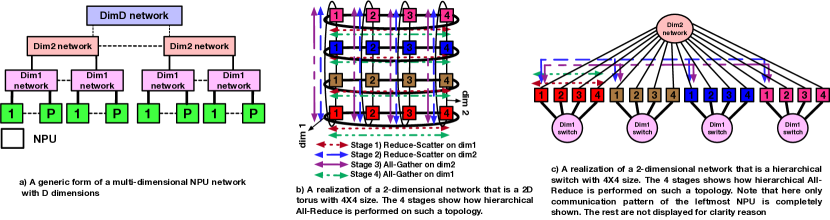
Figure 1. Distributed training platform with multi-dimensional interconnection networks. Usually, the lower dimensions have higher BW, as indicated by thicker lines in the figures. There are some exceptions such as Intel Habana Gaudi (int, 2016; Hab, 2019) platform, where multiple dimensions can be configured to have the same BWs.

Distributed Training Platforms. The challenge of training AI models has opened up a sub-field of systems research specifically aimed at designing efficient acceleration platforms for distributed training. These platforms are built by connecting tens of high-performance accelerators (e.g., GPUs or TPUs, which we call Neural Processing Units (NPU)) together. To leverage the compute capabilities of these platforms, the training workload (model + dataset) needs to be sharded across the accelerators via a parallelization strategy. The two most popular parallelization strategies are: (i) data-parallel, where a mini-batch is split, and (ii) model parallel, where a model is divided across NPUs. Recent efforts have also looked into hybrid (Naumov et al., 2019) and pipelined (Huang et al., 2019; Harlap et al., 2018) parallelization strategies.

We identify two key trends in the network architecture of the next-generation training platforms (int, 2016; NVI, 2021; Yasaman Ghadar and Tim Williams, 2020; Hab, 2019; Gra, 2016).

(i) The high number of network dimensions. Training platforms are built hierarchically. SOTA platforms today (dgx, 2019; goo, 2018) typically employ 2D network topologies — high BW proprietary links such as XeLink (Int, 2019) or NVlink (Li et al., 2019b) to interconnect NPUs on the same server followed by scaling out via NICs connected to ethernet or InfiniBand (Mel, 2020; NIC, 2021; Ethernet Technology Consortium, 2020). Fig. 1.a shows the abstraction of such a multi-dimensional network. Fig. 1.b and Fig. 1.c are two realizations of such platforms, resembling today’s torus-based (goo, 2018) and switch-based (dgx, 2019) topologies, respectively.

Next-generation platforms are expected to include multiple network dimensions. The reason for this is the growing compute and memory demand for ML models (Tra, 2021), which necessitates adding more NPUs. Adding more network dimensions is a natural way to increase scalability and overall BW per each NPU (int, 2016; Rashidi et al., 2021). Further, a suite of interconnect technologies is being developed to enable scalability. For instance, there is growing interest in (i) multi-chip packaging technologies to connect several NPU dies on a package (Shao et al., 2019; Amd, 2021; Rashidi et al., 2021; Arunkumar et al., 2017), (ii) high-bandwidth rack-scale interconnects (NVLink (NVL, 2022) from NVIDIA, XeLink (Int, 2019) from Intel, Infinity Fabric (AMD, 2021) from AMD) to connect NPU packages together, and (iii) high-speed NICs and switches (e.g., Mellanox SHARP (Mel, 2020)) to drive high-bandwidth over Infiniband or Ethernet.

(ii) Heterogeneity in the bandwidth of each dimension. Generally, network bandwidth (BW) decreases as we go to the next network dimensions. However, due to recent technological advancements, the overall BW across different network dimensions can be within a comparable range. Multi-chip packaging technology allows from 400 Gbps (Shao et al., 2019) to 3200 Gbps (Rashidi et al., 2021; Amd, 2021) BW per NPU (for NPU-to-NPU communication within a package). The rack-scale interconnect provides up to 3600 Gbps (NVL, 2022). Moreover, recently 400 Gbps NICs are introduced (NIC, 2021), and 800 Gbps NICs will be available in the near future (Ethernet Technology Consortium, 2020). Hence, the BW difference of the first-to-last dimension can be within 0.5–4$\times$.

These two trends lead to a challenge that this work identifies: maintaining high BW utilization across all network dimensions. This is due to the nature of collective communication patterns observed in distributed training. State-of-the-art collective communication (e.g., All-Reduce) scheduling algorithms use hierarchical algorithms, breaking the collective into phases (e.g., All-Reduce broken into Reduce-Scatter and All-Gather) and chunks from various phases of the collective moving through the network dimensions in a pipelined manner (Sec. 2.3). Unfortunately, as we identify in this work, a mismatch between the chunk (scheduling unit) size and BW per dimension can lead to unbalanced pipeline stages. This in turn means that the overall communication performance is dictated by the slowest stage, leading to network BW underutilization in other dimensions of the topology. This mismatch arises because the volume of data being sent per dimension depends on the workload (i.e., the DNN model being trained, its parallelism strategy, collective algorithm, and collective scheduling) while the bandwidth per dimension depends on system size, dollar costs, and other constraints (e.g., performance, cabling, power, etc.). While this is not a major problem in systems today which use few dimensions with significant BW gap across dimensions, this can lead to severe network BW underutilization for next-gen platforms with the characteristics described earlier.

In this paper, we propose Themis , a novel chunk scheduling scheme that dynamically gives different chunks distinct pipeline schedules to maximize the utilization of all network dimensions. We leverage the insight that algorithmically there is no strict ordering to perform Reduce-Scatter or All-Gather stages. In other words, to perform Reduce-Scatter/All-Gather stages a chunk may start at any network dimension and traverse dimensions in any order. The only synchronization point is that the Reduce-Scatter stage must be completed before starting All-Gather. Themis uses this fact and schedules chunks differently to balance loads of all network dimensions. Having intelligent schedulers like Themis is a key enabler for building next-gen platforms, letting system designers design the network with respect to their metrics (e.g, cost, performance), without concerning how to efficiently utilize the network BW.

In short, we make the following contributions:

• This is the first work, to the best of our knowledge, exploring the problem of multi-rail collective-communication scheduling at scale (1024 NPUs in this case) over next-gen hierarchical topologies.

• This is the first work to identify the problem of unbalanced stage latencies in multi-rail collective scheduling algorithms and show why this leads to BW underutilization for next-gen platforms.

• We propose Themis, a novel chunk scheduling scheme for multi-dimensional networks that dynamically schedules the chunks to maximize the utilization of each dimension. Themis is the first method, to the best of our knowledge, that proposes dynamic scheduling for different chunks for maximum BW utilization.

• Our results (see Sec. 5 for methodology) show that, on average, Themis achieves 1.72$\times$ All-Reduce time speedup and 95.14% BW utilization. This improves end-to-end training latency for ResNet-152, GNMT, DLRM, and Transformer-1T by 1.49$\times$ (2.25$\times$ max), 1.30$\times$ (1.78$\times$ max), 1.30$\times$ (1.77$\times$ max), and 1.25$\times$ (1.53$\times$ max), respectively.

• Using our analysis of efficient scheduling, we formulate different scenarios regarding the network BW distribution and give insights to the network designers for efficient BW distribution for the multi-dimensional networks tailored for large-scale training.

2. Background

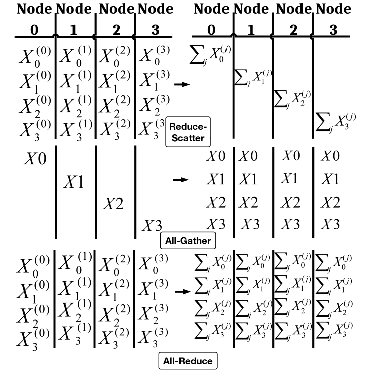
Figure 2. The Mathematical Implications of the Reduce-Scatter, All-Gather, and All-Reduce patterns executing on four NPUs. The left part shows the initial data on each communicating NPU before the collective operation. The right part shows data residing on each NPU after the completion of the collective operation.

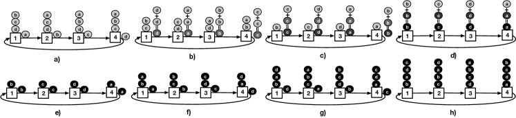
Figure 3. An example of the ring All-Reduce algorithm to perform the All-Reduce pattern. Steps a-d perform Reduce-Scatter pattern and steps e-g perform All-Gather pattern. Step h shows the final result.

2.1. Collective Communication Patterns

Communication is the inevitable overhead to pay in distributed training workloads. The exact communication patterns each training workload requires depend on the parallelization strategy, and also the communication mechanism (i.e. parameter server vs. explicit NPU-to-NPU). When using explicit NPU-to-NPU communication mechanisms, All-Reduce is the most dominant pattern observed in distributed training (Klenk et al., 2020).

AR can be broken into a Reduce-Scatter (RS) followed by an All-Gather (AG) communication pattern. Fig. 2 shows the mathematical implications of these patterns performed on four NPUs. RS performs reduction among initial data such that at the end, each NPU holds a portion of the globally reduced data. AG, on the other hand, broadcasts data residing on each NPU to all other NPUs. Therefore, it is clear that when performing RS/AG on $P$ participating NPUs, the data size residing on each NPU shrinks/multiplies by $P\times$.

Table 1. Topology options per dimension and corresponding contention-free topology-aware All-Reduce algorithms.

Topology	Topology-aware Collective
Ring	Ring (Thakur et al., 2005)
FullyConnected	Direct (Thakur et al., 2005)
Switch	HalvingDoubling (Dong et al., 2020)

2.2. Basic Collective Communication Algorithms

Each of the collective communication patterns described in Sec. 2.1 can be performed through different collective communication algorithms. For example, tree-based (Patarasuk and Yuan, 2009), ring-based (Chan et al., 2006), and halving-doubling (Dong et al., 2020) algorithms are proposed to realize AR pattern and are implemented in communication frameworks such as Intel oneCCL (Intel, 2020) or NVIDIA NCCL (ncc, 2017). Fig. 3 shows an example of the ring-based AR algorithm running on four NPUs.

The optimal collective algorithm is usually dependent on the physical topology and communication size (Thakur et al., 2005). For example, ring-based collective algorithms are a natural fit for NPUs connected via a physical ring, as it leads to zero contention. Table 1 presents some topology-aware collective algorithms, which are typically chosen dynamically by communication libraries (Intel, 2020; ncc, 2017) depending on the underlying topology. Such basic collective algorithms provide a basis to design more complex and tuned algorithms that are optimized for multi-dimensional network topologies, as we describe next.

2.3. Multi-Rail Hierarchical Collective Comm. Algorithms

As stated in Sec. 2.2, the optimal collective algorithm depends on the physical topology. Hence, the basic algorithms are not a good fit when having multi-dimensional physical networks with variable BW and latencies in each dimension. This is because the collective algorithms are inherently synchronous and in this case, the links with the least BW will become the bottleneck, making other high-BW links underutilized. To cope with this, recent works propose multi-rail hierarchical algorithms to exploit different dimensions’ BW and latency (Cho et al., 2019; Wang et al., 2020). Suppose the topology has $D$ dimensions as shown in Fig. 1.a, the AR algorithm breaks into the following 2$\times$D pipeline stage scheduling:

• A sequence of RS stages starting from dim1 and ending at dim$D$ ($D$ stages in total). After these stages, data is globally Reduce-Scattered across all NPUs.

• Next, a sequence of AG stages are performed in the reverse order ($D$ stages in total); starting from dim$D$ and ending at dim1.

The above order is the baseline collective scheduling, used by SOTA collective libraries today (Wang et al., 2020; Cho et al., 2019). The main reason for such hierarchical phases is to reduce traffic as the collective goes to the next dimension, which usually has lower BW compared to the previous dimension. The RS/AG algorithm for each stage is a basic topology-aware collective (Sec. 2.2) and is independently selected by the collective scheduler (Cho et al., 2019; Intel, 2020). For example, a topology with rings in the first and switches in the second dimension may run a series of RS/AG stages using ring-based and halving-doubling algorithms, respectively.

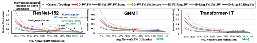
Figure 4. Normalized runtime vs. average BW utilization for three different-sized DNN training workloads running on a current topology, a 2-dimensional topology with the characteristics similar to (dgx, 2019), and six different next-gen topologies (please see Sec. 5 for full description of workloads and topologies). The DNNs are: (i) ResNet-152, (ii) GNMT, and (iii) Transformer-1T (1 Trillion params). The avg. BW utilization is the weighted average of BW utilization across all dimensions of the network, with respect to the BW budget of each dimension (i.e., dimensions with higher BW get higher weight). It is obtained only during the time when there are communication operations issued by the workload (excluding the times when there is no pending communication operation). All runtimes are normalized to the slowest topology (i.e., current topology) runtime at 10% BW utilization. The bold dots show the BW utilization when the multi-rail hierarchical algorithm with baseline scheduling (discussed in Sec. 2.3) is used. Inf (i.e., infinite) BW is when communication overhead is 0% and runtime stems from compute only. The ideal is the achievable runtime if the network BW across all dimensions is fully utilized. For a fair comparison of network performance, we assume all systems use the same compute model (Sec. 5).

Fig. 1.b and Fig. 1.c show two examples of how this AR algorithm is applied on a 2-dimensional network. In both examples, the first dimension comprises the NPUs with the same color, meaning that the peer NPUs for the communication is the NPUs with the same color. The second dimension is shown based on the NPUs with the same number. Throughout this paper, we use the notation $P_{1}\times P_{2}\times....\times P_{D}$ to refer to the size of a multi-dimensional network where $P_{i}$ is a number referring to the size of peer NPUs participating in the communication on the i’th dimension. For example, the size of both Fig. 1.b and Fig. 1.c is $4\times 4$.

Chunks. Communication data is usually broken into multiple chunks (Cowan et al., 2022; Shah et al., 2021; Luo et al., 2020) and then these chunks are fed into this 2$\times$D-stage pipeline to keep all dimensions busy. A chunk is a portion of data to participate in the collective, and the collective algorithm can work on each chunk independently. For example, a 256MB AR can be broken into four independent chunks of 64MB All-Reduces. In this paper, we assume the size of each chunk in each stage to be the size of the corresponding chunk data residing on each NPU before the stage begins. Similar to the explanation of Sec. 2.1, each chunk size changes after each stage of RS/AG.

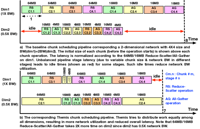
Figure 5. The execution of a 256MB All-Reduce running on a 4$\times$4 2-dimensional network where BW(dim1)=2BW(dim2). The All-Reduce is broken into 4$\times$64MB chunks.

3. Motivation - Network BW underutilization

As discussed in Sec. 2.3, hierarchical collectives are the SOTA method for the multi-dimensional networks with variable BW. However, we identify that reaching the maximum possible network utilization is quite challenging for next-gen platforms.

Definition: Average BW Utilization. We define avg. BW utilization is the weighted average of BW utilization across all dimensions of the network, with respect to the BW budget of each dimension (i.e., dimensions with higher BW get higher weight). In the case of real workloads, it is estimated only during the time when there are communication operations issued by the workload (excluding the times when there is no pending communication operation due to compute/memory operations (Rashidi et al., 2021)).

3.1. Next-Gen Distributed Training Platforms

Today’s high-end training platforms typically use 2-dimensional topologies (dgx, 2019; Mudigere et al., 2021) – one to connect several NPUs within the same server node together using high-speed proprietary links (Int, 2019; NVL, 2022) – followed by node-to-node communication via Network Interface Cards (NICs). We model such 2D networks but with high bandwidth across both dimensions as a result of recent technology advancements (such as Intel’s XeLink (Int, 2019), NVIDIA’s NVlink (NVL, 2022)) and high-speed NICs (NIC, 2021; Ethernet Technology Consortium, 2020) on next-gen platforms.

However, as workload model sizes increase (Vaswani et al., 2017), the need for more NPUs and higher communication bandwidth increases. There is thus a growing industry trend (Nvi, 2022; Hab, 2019; Yasaman Ghadar and Tim Williams, 2020; NVI, 2021; Gra, 2016; Int, 2022) to increase the number of dimensions before getting to the NIC to reduce the NIC traffic. We model multiple such futuristic 3-dimensional training platforms in this work as described in Table 2. The first dimension (dim1) represents the intra-node dimension where NPUs on the same server node are connected through a high-BW rack-scale fabric. Several nodes are then connected by allocating a portion of the rack-scale fabric to create pod (dim2) (Nvi, 2022; Hab, 2019), again, using high-BW dedicated links. In the third dimension, NPUs within dim2 are connected to the dim3 switches through NICs. 4-dimensional topologies extend the 3D topologies by adding Multi-Chip packaging (Arunkumar et al., 2017; Shao et al., 2019) as the first dimension to incorporate multiple NPUs within a package (Arunkumar et al., 2017; AMD, 2021; Rashidi et al., 2021). Sec. 5 provides more details of our methodology for modeling these platforms.

3.2. Quantifying Network BW Underutilization

Fig. 4 shows the overall (normalized) training time reduction as the avg. network BW utilization increases for three different DNNs with a high ratio of communication to compute. The modeled platforms are a suite of 2D, 3D, and 4D topologies as explained in Sec. 3.1 and Table 2. Each line in Fig. 4 shows the normalized runtime (y-axis) for different BW utilization (x-axis) of a specific topology. The runtime curves are relatively similar across the three training workloads. This is because these workloads are communication bound, hence, their runtime is mainly dictated by the underlying network performance.

As Fig. 4 shows, adding more network dimensions usually results in lower end-to-end training runtime, due to increased network BW per NPU. This is the motivation for the next-generation training platforms to add more network dimensions. However, the overall network BW utilization starts to drop as we add more dimensions and/or have high BW across all network dimensions, as we discuss next.

We observe from Fig. 4 that a current topology can achieve 97.7% BW utilization with the baseline collective scheduling policy as discussed in Sec. 2.3. This is primarily due to the huge BW difference between dim1 and dim2 (i.e. 1200 Gbps vs. 100 Gbps), making underutilization of dim2 play an insignificant role in overall performance. However, as stated earlier, next-gen platforms have high BW across dimensions, as well as having more network dimensions.

Fig. 4 also shows how baseline collective communication scheduling fails to efficiently utilize the available BW on these next-gen topologies, reaching the average BW utilization of 59.7% (35.1% min), when averaging across all the workloads and topologies. To obtain linear (perfect) speedup as we scale the number of NPUs for training, the communication overhead should remain 0% (the Inf BW case in Fig. 4). However, this is not feasible due to finite network BW resources (technology constrained in each dimension). Hence, for a given topology, the maximum achievable speedup is when BW utilization is 100% (“Ideal" in Fig. 4), and any network underutilization diminishes the benefits of scaling. For the next-gen topologies, if the ideal utilization (100%) can be achieved, the training performance on average can be improved by 1.54$\times$ (2.34$\times$ max), 1.32$\times$ (1.81$\times$ max), and 1.26$\times$ (1.54$\times$ max) over the baseline for ResNet-152, GNMT, and Transformer-1T, respectively.

3.3. Understanding Network BW Underutilization

To illustrate the problem, Fig. 5.a shows how a 256MB baseline hierarchical AR is performed on a 2-dimensional network with the second dimension having half BW of the first dimension. The collective is broken into 4$\times$64MB chunks. There are 4 pipeline stages for performing hierarchical AR on this network: ① RS on dim1, ② RS on dim2, ③ AG on dim2, ④ AG on dim1.

A 64MB chunk size will be shrunk by 4$\times$ when entering stage 2, meaning that RS on the stage injects $\frac{1}{4}\times$ data to the dim2 compared to the stage 1 injecting to dim1. However, dim2 has $\frac{1}{2}\times$ BW compared to the dim1. If we assume the 64MB RS (or 16MB AG) takes 1 unit of time when running on dim1, then the latency of that chunk for the stage 2 is:$\frac{0.25Data}{0.5BW}=0.5$. Therefore, stage 2 is performing 2$\times$ faster than stage 1. Stage 3 injects the same amount of data as stage 2 and operates on the same dimension, hence its latency is similar to stage 2. Using the same argument, stage 4 has the same latency as stage 1. The faster processing of stage 2 and stage 3 means they are underutilized many times. This indicates that their corresponding network dimension (i.e. dim2) is underutilized as shown in Fig. 5.a.

We note that the only place where the baseline algorithm can reach near 100$\%$ utilization is when the BW reduction ratio in the next dimension is proportional to the size of the current dimension. Again, consider the $4\times 4$ system size. For the baseline system to be efficient, the BW(dim1)=4$\times$BW(dim2) because dim1 shrinks the chunk size by $4\times$. It is only in this case that stage latencies will be equal using the baseline algorithm. Any excess BW of dim2 beyond this point will be wasted, as when we show in Fig. 5.a where BW(dim1)=2BW(dim2).

In general, this concept can be generalized to any D-dimensional network of size $P_{1}\times P_{2}\times....\times P_{D}$. For the baseline to be efficient, we must have:

$\text{BW(dim1)}=P_{1}\times\text{BW(dim2)}=P_{1}\times P_{2}\times\text{BW(dim3)}=...=P_{1}\times P_{2}\times....\times P_{D-1}\times\text{BW(dimD)}$.

However, this creates an unpleasant requirement for the network as a result of the poor scheduling of the baseline algorithm. If we plug the above formula for the current platform (discussed in Fig. 4), we find out that all dim1 BW (1200 Gbps) and 75 Gbps (out of 100 Gbps) of dim2 are utilized using baseline collective scheduling, justifying its high BW utilization in Fig. 4. But the underlying network dimensions can have more BW available in next-gen systems and the algorithm must be able to utilize excess BW provided by the network dimensions.

Note that in the above example, our analysis was based on the assumption that the network BW is the primary factor that determines communication latency (which is true for large collectives). However, the concept of unbalanced stage latencies remains true even if we take into account other factors (e.g. link latency) as we show in Sec. 4 and Sec. 6. We also wish to emphasize that the underutilization we are referring to is a fundamental challenge due to chunk size and bandwidth mismatch (as our example indicated) and not due to any network stalls because of compute/memory bottlenecks that limit network performance (Rashidi et al., 2021; Klenk et al., 2020) (which may further exacerbate this issue) but are not the focus of this work.

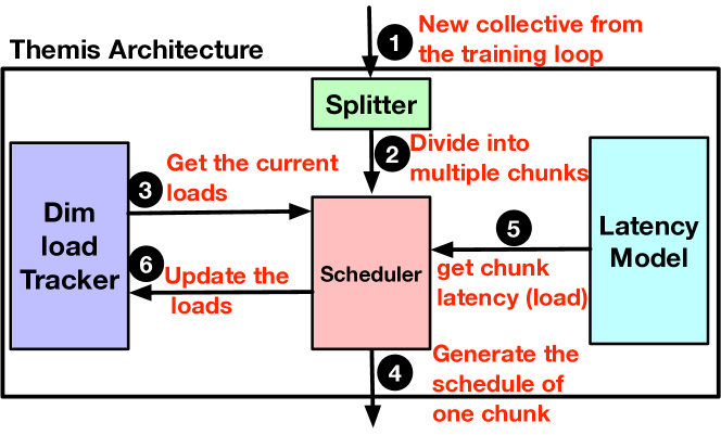
Figure 6. An overview of Themis components. 1) A collective operation is requested from the upper layer training workload. 2) The collective is split into multiple equal size chunks. Steps 3–6 are performed on an individual chunk basis. 3) the current load of network dimensions (in terms of total communication latency) is retrieved from the Dim Load Tracker. 4) Scheduler sorts the dimension loads in ascending/descending orders and the sorted list order is the schedule for the current chunk through the Latency Model. 5) Based on the schedule generated, Scheduler finds out the latency of the new schedule for each dimension. 6) Scheduler updates the total loads of each dimension to take into account the load of the new chunk.

Algorithm 1 Themis Algorithm

Inputs: CollectiveType ($CT$), CollectiveSize ($CS$), ChunksPerCollective ($CPC$), TotalNPUs ($P$)

Output: A 2D list $Schedule[][]$ where $Schedule[i][]$ gives the order of dimensions the i’th chunk should traverse for the collective.

1:procedure Schedule_Collective($CT,CS,CPC$)

2:     DimLoadTracker.reset($CT$)

3:     ChunkSize=$CS/CPC$

4:     i=0

5:     for i++ < $CPC$ do

6:         if $CT==\text{All-Reduce}$ then

7:              RS_Sch=SCHEDULER.SCHEDULE($RS,ChunkSize$)

8:              AG_Sch=reverseOrder($RS\_Sch$)

9:              $Schedule[i][]$=concatenate(RS_Sch, AG_Sch)

10:         else

11:              $Schedule[i][]$=SCHEDULER.SCHEDULE(

12:                                                  $CT$, ChunkSize)

13:         end if

14:     end for

15:     return $Schedule$

16:end procedure

17:procedure Scheduler.Schedule($CT,ChunkSize$)$\triangleright$ Schedules a chunk

18:     loads=DimLoadTracker.getLoads()

19:     if loads.max_dim_load - loads.min_dim_load $<$ Threshold then

20:         schedule=getBaselineScheduling($CT$)

21:     else

22:         if $CT==\text{Reduce-Scatter}$ then

23:              schedule=getIndexOfSortedList($loads,ascending$)

24:         else if $CT==\text{All-Gather}$ then

25:              schedule=getIndexOfSortedList($loads,descending$)

26:         end if

27:     end if

28:     newLoad=LatencyModel.calcLoads(

29:                                      $chunkSize,schedule,CT$)

30:     DimLoadTracker.update(newLoad)

31:     return schedule

32:end procedure

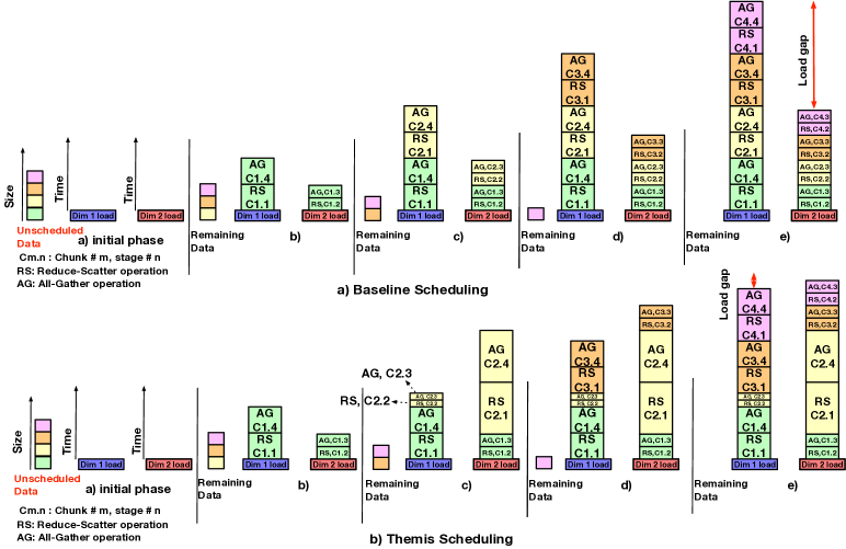
Figure 7. An example of Baseline Scheduling vs. Themis Scheduling corresponding to the chunk scheduling problem of Fig. 5. Each of the steps b-d shows scheduling for one chunk. Dim load shows the total communication time of each dimension. As shown in the figure, baseline scheduling always uses a constant schedule for all chunks, resulting in the underutilization of abundant BW provided by dim2. However, Themis uses a greedy scheme to schedule new chunks in a way that puts more load on the dimensions with lower loads. In Themis: step b) all dim loads are zero, thus, the first chunk schedule is similar to the baseline. In step c) dim2 has a lower load, hence the chunk scheduling starts from dim2 to fill the gap with dim1. In step d) and step e) Chunk schedule starts from dim1 to fill the gap with the overloaded dim2.

4. Themis

In this section, we present Themis that performs dynamic and distinct scheduling for each chunk to balance the loads across different network dimensions. Themis is specifically designed to maximize the multi-dimensional network BW for All-Reduce (AR), Reduce-Scatter (RS), and All-Gather (AG).

4.1. Themis Intuition and Overview

Themis has its roots in two main observations:

Observation 1. From the algorithm’s correctness point of view, there is no restriction on how each chunk should traverse the RS/AG stages. For example, in the case of AR on a 2D network explained in Sec. 3, the RS stage on the second dimension can precede the RS on the first stage. Similar ordering independence is true for AG stages. Furthermore, the ordering of RS stages can be different than AG stages. The only synchronization point is that the RS stages should be finished before starting the AG stages. Thus, the following 4 different schedules are all possible for the AR collective on a 2D topology:

1. (i) RS on dim1, (ii) RS on dim2, (iii) AG on dim2, (iv) AG on dim1 (this is the baseline scheduling).

2. (i) RS on dim2, (ii) RS on dim1, (iii) AG on dim2, (iv) AG on dim1.

3. (i) RS on dim1, (ii) RS on dim2, (iii) AG on dim1, (iv) AG on dim2.

4. (i) RS on dim2, (ii) RS on dim1, (iii) AG on dim1, (iv) AG on dim2.

In general, for any D-dimensional network, there are $D!\times D!$ valid ways to schedule an AR data chunk ($D!$ for RS/AG only).

Observation 2. Different chunks can have different schedules. Hence, if we divide a collective into C chunks, the space of all possible schedules for all chunks on an N-dimensional network is $(D!\times D!)^{C}$ for AR ($D!^{C}$ for RS/AG), indicating the exponential growth as the network dimensions and the number of chunks increase. Together, observation 1 and observation 2 motivate the Themis idea which is to independently schedule chunks across network dimensions based on the available bandwidth, rather than following a strict order like previous works (ncc, 2017; Cho et al., 2019; Wang et al., 2020). For each dimension, each chunk uses the topology-aware collective algorithm for that dimension (Sec. 2.3), just like the baseline hierarchical algorithm.

Themis Overview. Fig. 6 shows the general overview of Themis. Splitter component simply divides the collective into multiple equally-sized chunks. Dim Load Tracker maintains the load of each network dimension in terms of the total communication time of the chunks when executing on that dimension. The Latency Model predicts the RS/AG communication time for a given chunk size running on any network dimension. Finally, Scheduler generates a dynamic schedule for each chunk based on the information provided by the Dim Load Tracker and Latency Model. Fig. 6 also shows the series of steps when a new collective communication is issued from the training workload layer. We describe its workflow next.

4.2. Themis Algorithm

In Sec. 4.1 we showed how the space of available schedules grows exponentially. Therefore, it is not practical to search all possible schedules, even for modest network and chunks granularity. Instead, Themis is a type of greedy algorithm that tries to schedule new chunks in a way that puts more load (in terms of communication time) on the dimension with an already lower load. Themis leverages the two observations explained in Sec. 4.1 for more flexible scheduling. Algorithm 1 shows the pseudo-code for Themis. The SCHEDULE_COLLECTIVE procedure (line 1) is called whenever a new collective is requested by the training workload. Lines 2–4 are for initialization. The for loop in line 5 is for chunking the data while the lines 6–13 are executed to call the scheduler to determine the schedule of each chunk through SCHEDULER.SCHEDULE procedure. Note that Themis assumes the AG schedule is the reverse order of obtained RS schedule for a chunk if the collective is AR (line 8). The scheduler first retrieves the current loads of all network dimensions via the Dim Load Tracker component (line 18). Dim Load Tracker is simply a list that contains the total load (chunk runtimes predicted by the Latency Model) that is placed on each dimension by the current schedules of the chunks. Lines 19–21 are for the robustness of Themis and check if the current load difference between the dimensions with maximum and minimum load is below a threshold. If this is true, then Themis reverts to the baseline scheduling to prevent oversubscribing the network dimensions with lower BW just because their current load is slightly lower than the dimensions with higher BW. If the condition of line 19 is false, Themis schedules the current chunk in a way to balance the loads across different dimensions. It first gets the index of dimensions sorted from least (most) load to most (least) load if the collective type is RS (AG) (lines 21–27). This sorted list is the schedule for the new chunk, since such a schedule puts more load on the dimensions with currently lower loads, leading to filling the gap between the high-load and low-load dimensions. Next, the Latency Model predicts the load of the newly scheduled chunk (lines 28–29), and then Dim Load Tracker is updated (increased) accordingly (line 30). The Latency Model is a function that inputs chunk size, network dimension, and chunk operation (RS/AG), and returns the predicted runtime for that chunk operation running on the specific dimension. Then, the scheduling process for the next chunk begins.

Example. Fig. 7 shows how baseline vs. Themis scheduling works (i.e. assigns schedules) for the example of Fig. 5. As Fig. 7 shows, the baseline scheduling scheme always assigns a constant schedule for all chunks, hence, the gap between dim1 and dim2 preserves as new chunks are scheduled. However, Themis schedules the chunks differently to balance the dimension loads. In this example, Themis schedules the second chunk to start from dim2 to fill the gap between dim1 and dim2 (step c). After that, the last two chunks start from dim1 to fill the gap of dim1 with now overloaded dim2 (steps d&e). Fig. 5.b shows the Themis time diagram that is based on the schedule generated in Fig. 7.b. As Fig. 5.b shows, such dimension load balancing results in better network utilization and reduced total communication time. We used a 2-dimensional example for simplicity. However, in general, the lack of ability to utilize the network BW in the baseline scheduling is more pronounced as the number of network dimensions and available extra BW of dimensions increase.

4.3. Intra-Dimension Chunk Scheduling

So far, we have discussed how Themis schedules chunks across different dimensions to balance the loads (inter-dimension scheduling). Another question to answer is how different chunks within a dimension are ordered for processing because at any given point there might be multiple chunks available for each dimension. Adverse intra-dimension scheduling can lead to starvation of some dimensions since their, yet to come, chunks are stuck within the queues of other dimensions.

We found out that in the baseline scheduling scheme, intra-dimension scheduling has minimal effects on the performance due to the identical schedule of all chunks. In other words, no matter how each dimension selects chunks to process, the average BW utilization remains fixed. The only difference is in the periods of time where the dimensions are utilized. Moreover, a monotonic schedule means each network dimension always receives the same chunk sizes. Hence, we assume the baseline scheme uses a simple FIFO-based intra-dimension chunk execution.

But for Themis, chunk intra-scheduling is important due to the different schedules of chunks, that result in variable chunk sizes per dimension. We empirically found the best policy to be Smallest-Chunk-First (SCF). The underlying intuition is that processing smaller chunks takes a shorter time and allows the chunk to be fed to other dimensions faster. This reduces the chance of a network dimension momentarily being idle due to not having collective chunks to process (i.e., dimension starvation).

Also note that if the chunk is small, processing one chunk per dimension underutilizes the network BW since small messages cannot saturate the given BW (e.g., due to the link latency). Hence, in this case, multiple chunks per dimension (if available) should be run in parallel to fully saturate a dimension’s available BW (similar to the collective fusion concept in NCCL (ncc, 2017)).

4.4. Understanding All Latency Parameters

The techniques presented in Sec. 4.2 and Sec. 4.3 aim to balance the total latency across different network dimensions, since the collective performance is dictated by the slowest dimension. In general, the total latency of the K’th network dimension (dimK) can be calculated as follows:

$$\textit{Latency(dimK)}=A_{K}+(N_{K}\times B_{K})+idle_{K}$$

While $A_{K}$ refers to the fixed delay caused by the collective algorithm and system latencies, $N_{K}$ is the total amount of bytes scheduled, $B_{K}$ is the per-byte latency, and $idle_{K}$ is the idle time, all corresponding to dimK. Among these parameters, $A_{K}$ and $B_{K}$ are given by the system specification and/or collective algorithm, while Themis controls $N_{K}$ and $idle_{K}$.

$A_{K}$ is the fixed delay to pay to run a certain collective type on a network dimension and is determined by:

$$A_{K}=\text{number\_of\_steps}\times\text{step\_latency}$$

number_of_steps is determined by the basic collective communication algorithm (Sec. 2.2) employed on dimK. For example, ring-based All-Reduce require $2P_{K}-2$ steps on dimK. On the other hand, step_latency is determined by the network component latencies (e.g., NIC latency, link latency, etc.) when transferring a minimum-size message between two NPUs (Shah et al., 2021). On real systems, $A_{K}$ can be calculated by running a minimum size collective on dimK.

To account for this delay in Themis, the Dim Load Tracker initializes each dimension’s load to its respective $A_{K}$ for the target collective type (line 2 in Algorithm 1). Note that $A_{K}$ of different dimensions are considered to be negligible and not shown in the example of Fig. 7 for more readability.

The per-byte latency ($B_{K}$) is directly proportional to the inverse of link BW (Cai et al., 2021), while $N_{K}$ corresponds to the total data size each NPU sends out on dimK and is calculated as follows:

$$N_{K}=\sum_{i=1}^{CPC}n_{K}^{i}$$

Where $n_{K}^{i}$ is the total amount of data each NPU sends out on dimK to process chunk #i with respect to its schedule and collective algorithm .

Effectively, Themis (Sec. 4.2) controls $N_{K}$, through dynamic scheduling of chunks, to balance the overall latency across different dimensions. Since $N_{K}$ only participates with $B_{K}$, the Latency Model only considers $n_{K}^{i}\times B_{K}$ as the latency of chunk #i on dimK (lines 28–29 in Algorithm 1).

The other factor is $idle_{k}$ that corresponds to the times where dimK network is idle, while there are other chunks stuck on other dimensions and yet have some pending stages on dimK to be executed later. To minimize the $idle_{k}$, we make 2 provisions as described in Sec. 4.3. First, we employ SCF intra-dimension chunk scheduling to reduce the chance of dimension starvation. Second, if multiple available chunks are available, we execute multiple chunks per dimension if one chunk cannot fully saturate the network BW.

4.5. Supporting In-Network Collective Offload

In recent years, several works have shown the communication performance improvement by offloading collectives to the switches belonging to different network dimensions (Klenk et al., 2020; Li et al., 2019a; Nvi, 2022; De Sensi et al., 2021). Switch collective offload reduces the collective’s network traffic (i.e., $n_{K}^{i}$) and fixed delay (i.e., $A_{K}$) (De Sensi et al., 2021). However, the concept of running hierarchical collectives, as described in Sec. 2.3, to cope with the heterogeneous multi-dimensional networks remains the same. Hierarchical collectives may suffer from the imbalanced network dimension loads as we discussed throughout this paper. Therefore, Themis can be used to balance the loads across different network dimensions even when in-network collective is available.

4.6. Chunk Schedule Consistency

To design a distributed chunk scheduling algorithm, it is important that all NPUs execute the same order of chunks operations on their different dimensions. Failing to do so can lead to chunk schedule inconsistency and create a deadlock, since different NPUs wait on executing different chunk operations, and hence, no chunk can proceed (ncc, 2017). To maintain consistency, we must make sure that: (i) all NPUs produce the same chunk schedule (Inter-Dimension Schedule Consistency) and (ii) for a given dimension, all NPUs execute the same order of chunk operations (Intra-Dimension Schedule Consistency).

4.6.1. Inter-Dimension Schedule Consistency

Inter-dimension schedule consistency is guaranteed since both the Latency Model and Dim Load Tracker are similar across all NPUs, and behave in the same way as explained in Sec. 4.4. This is possible because both $A_{K}$ and $B_{K}$ parameters can be obtained offline and replicated across all NPUs. Therefore, different NPUs produce exactly the same schedule for the chunks of a collective operation.

Table 2. List of target topologies and their BW/latency configurations per each dimension. The naming convention starts with the number of dimensions followed by dimension topology time in increasing order. For example, 3D-FC_Ring_SW means a 3-dim topology where dim1 is FullyConnected, dim2 is Ring, and dim3 is Switch. Each color shows a dimension in which the network connects the NPUs together. The BW and latency in each dimension are selected according to the predicted ranges for link technologies in the future systems, listed below the table. We note that based on technology trends, there is a wide range of BW and latency options for each dimension depending on the technology and other constraints. All combinations cannot be presented here due to the lack of space. We create a diverse set of topologies with a different BW ratio to motivate the problem and demonstrate the applicability of Themis on various platforms. The Aggr BW/NPU is the product of the BW/link determined by the technology and Links/NPU is determined by the topology.

Name	NPUs	Size	BW/Link (Gb/s)**	#Links/NPU	Aggr BW/NPU (Gb/s)	Network Latency (ns)**
2D-SW_SW	1024	16$\times$64	(200, 800)	(6, 1)	(1200, 800)	(700, 1700)
3D-SW_SW_SW_homo	1024	16$\times$8$\times$8	(200, 200, 800)	(4, 4, 1)	(800, 800, 800)	(700, 700, 1700)
3D-SW_SW_SW_hetero	1024	16$\times$8$\times$8	(200, 200, 400)	(8, 4, 1)	(1600, 800, 400)	(700, 700, 1700)
3D-FC_Ring_SW	1024	8$\times$16$\times$8	(200, 200, 400)	(7, 4, 1)	(1400, 800, 400)	(700, 700, 1700)
4D-Ring_SW_SW_SW	1024	4$\times$4$\times$8$\times$8	(1000, 200, 200, 400)	(2, 8, 4, 1)	(2000, 1600, 800, 400)	(20, 700, 700, 1700)
4D-Ring_FC_Ring_SW	1024	4$\times$8$\times$4$\times$8	(1500, 200, 200, 800)	(2, 7, 6, 1)	(3000, 1400, 1200, 800)	(20, 700, 700, 1700)

**Link Technologies for each Dimension: chiplet-to-chiplet (within a package)  (Arunkumar et al., 2017; Shao et al., 2019; AMD, 2021; Rashidi et al., 2021), package-to-package (within a server node) (NVL, 2022; Yasaman Ghadar and Tim Williams, 2020; Hab, 2019; Shah et al., 2021), node-to-node (Hab, 2019; NIC, 2021; Ethernet Technology Consortium, 2020; Shah et al., 2021), pod-to-pod. (NIC, 2021; Ethernet Technology Consortium, 2020; Cis, 2019; Shah et al., 2021). Note - for all topologies, the last dimension uses NICs, which is node-to-node for 2D, and pod-to-pod for 3D and 4D. The network latency (i.e., step_latency in Sec. 4.4) corresponds to the direct NPU-to-NPU latency when sending a minimum-length message.

4.6.2. Intra-Dimension Schedule Consistency

Runtime variation might rarely result in chunks being available for a given dimension in different orders across different NPUs. For example, suppose the chunk operations C1.1 and C2.1 are under execution on dim1 and dim3, respectively, and their next operation (i.e., C1.2, and C2.2) is scheduled on dim2. Runtime effects (e.g., packet drop, endpoint congestion) might cause C1.1 to slightly finish sooner than others, followed by the immediate start of C1.2 on dim2 on some NPUs. Now suppose on some NPUs with unfinished C1.1, C2.1 is finished sooner, and hence, those NPUs begin running C2.2 on dim2, creating a potential deadlock case.

To prevent this, once Inter-Dimension Schedules are determined (according to Sec. 4.6.1), Themis simulates their execution to get an estimation of when each chunk operation will be available on each dimension. Once chunk operation availability is estimated, Themis enforces this intra-dimension ordering on runtime. Even if some chunks are available sooner on the NPU, Themis does not execute them if it is not their turn to be executed.

Note that the simulation is deterministic, so all NPUs produce the same intra-dimension ordering. In addition, the simulation does not need to consider detailed network modeling and is performed fast, since the aim is the order of chunk availability on each dimension, and not their exact availability time. Once a certain collective schedule and its ordering are generated by Themis, it is saved and reused on later training iterations. So, there is no need to repeat the process in later training iterations.

Table 3. Target Collective Schedulers

Method	Comment
Baseline	Uses multi-rail hierarchical algorithm (Cho et al., 2019) as explained in Sec. 2.3 with FIFO intra dimension scheduling.
Themis+FIFO	Uses Themis with FIFO intra-dimension scheduling.
Themis+SCF	Uses Themis with SCF intra-dimension scheduling.
Ideal	Assumes 100% BW is utilized. Communication latency is simply calculated by (collective size / total BW).

5. Methodology

In this section, we provide our methodology and the target systems and workloads to evaluate Themis and baseline.

5.1. Simulation Platform

We use the ASTRA-SIM simulator (Ast, 2020; Rashidi et al., 2020b) to implement our scheme and compare it with the baseline system. ASTRA-SIM provides the flexibility to define various large-scale hierarchical training platforms, enabling us to demonstrate the efficiency of Themis on future platforms. ASTRA-SIM simulates the communication performance of the distributed training workloads in detail. It supports heterogeneous networks, different collective communication algorithms, and different parallelization strategies. For compute times (in the case of real workloads) we assumed roofline FP16 performance from the total FLOPS available on current state-of-the-art accelerators (A10, 2020).

We note that, since we are targeting next-gen systems, using simulation as our evaluation methodology is our only option to show the necessity of Themis for such systems. Recall that regular topologies and hierarchical topology-aware collective communication algorithms (Sec. 2.2) per dimension lead to congestion-less network traffic, enabling detailed simulators to accurately model and match real system measurements for collectives (Ast, 2020; Rashidi et al., 2020b).

5.2. Training Platforms and Workloads

Table 2 shows our target topologies all consisting of 1024 NPUs to resemble large-scale next-generation systems. Sec. 3.1 presents more description of trends and previous works that leads to the topologies presented in Table 2. We do not consider in-network collective offload support due to the lack of space, although we expect Themis still improves the network BW utilization in this case, as explained in Sec. 4.5.

All-Reduce Algorithm. Table 1 lists the topology-aware and contention-free AR algorithms we employ.

Target Workloads and Parallelization. Themis is a solution to maximize the BW utilization of pervasive collective communications on multi-dimensional networks. Collective communication is an integral part of any synchronous training job with an NPU-to-NPU communication mechanism. Moreover, collective usage is not limited to training only, and has been widely used in other domains (e.g., in HPC applications and distributed inference). However, we limit the scope of our evaluations in this work to DL training given its importance.

For real workload training, we selected four DNNs from different domains of deep learning applications: ResNet-152 (He et al., 2015) (from computer vision), DLRM (Naumov et al., 2019) (from recommendation models), GNMT (Wu et al., 2016), and Transformer-1T (one trillion parameter) (Tra, 2021) (both from NLP domain). For DLRM, we use the model described in (Rashidi et al., 2020a). The gradient precision is FP16 in all workloads and the per-NPU minibatch size is set to be 32, 512, 128, and 16 for ResNet-152, DLRM, GNMT, and Transformer-1T, respectively. Such workloads have a high ratio of communication-to-computation and hence, benefit most from applying Themis.

In terms of parallelization strategy, ResNet-152 and GNMT use the complete data-parallel partitioning since they can fit within single NPU’s memory. DLRM uses data-parallel partitioning for its MLP layers, while its sparse features (embedding tables) are partitioned in model-parallel. To reduce the memory requirements for DNN training, Transformer-1T uses Microsoft ZeRO optimizer stage 2 (Rajbhandari et al., 2020). Transformer-1T is partitioned in a model-parallel manner across the first dimensions up to 128 NPUs, and data-parallel across the remaining dimensions. The reason is that a single NPU memory is usually within the range of 48–64GB (Hab, 2019; Yasaman Ghadar and Tim Williams, 2020). Thus, the entire parameters of Transformer-1T (even after applying ZeRO optimizer) can not fit on a single NPU, requiring model-parallel to split the model.

Multi-Tenancy. We target systems that are private training clusters dedicated to training a DNN workload at a time without other interfering workloads. Therefore, the NPU network only observes a single workload training traffic. Such platforms are common enough to be considered separately and are widely deployed in the industry to train critical workloads (Mudigere et al., 2021; goo, 2018; NVI, 2021).

5.3. Target Configurations

Target Scheduling Configurations. Table 3 shows the scheduling policies we implement. The baseline uses FIFO intra-dimension policy as different intra-dimension policies have no effect on its performance (discussed in Sec. 4.3).

To decompose the effect of inter-dimension and intra-dimension scheduling, we present two flavors of Themis: i) Themis+FIFO that uses the default FIFO intra-dimension scheduling policy, and ii) Themis+Smallest-Chunk-First (SCF) with optimized SCF intra-dimension policy. Moreover, for the real workloads, we implement an Ideal method that assumes 100% network BW utilization. The ideal method determines the upper bound for maximum achievable speed-up and guarantees that no chunk scheduling scheme can exceed its performance.

Themis Parameter Values. According to Fig. 6 and Algorithm 1, Themis has two important parameters to be set: the number of chunks per collective and the Threshold (line 19 in Algorithm 1). Unless mentioned otherwise, we set the number of chunks per collective to be 64 in all our experiments for both the baseline and Themis. We set the Threshold to be the estimated runtime (predicted by the Latency Model) when running an RS/AG of size $\frac{\text{chunkSize}}{16}$ on the dimension with the lowest current load.

6. Results

In Sec. 6.1, we first present the single collective microbenchmark results and dive deep into the reasons for Themis showing benefits over the baseline scheduling scheme. Next, in Sec. 6.2 we present the end-to-end training iteration results for real workloads such as ResNet-152, GNMT, DLRM, and Transformer-1T. Finally, in Sec. 6.3, we give insights on how next generation networks should be designed in terms of BW distribution for distributed training.

6.1. Microbenchmark Results

Fig. 8 shows the All-Reduce communication results of the baseline and Themis, ranging from 100 MB to 1 GB. We pick this range to represent the (relatively) large models’ collectives that are the target of such large-scale distributed training systems. This range also covers our target workloads collectives in Sec. 6.2.

As Fig. 8 shows, applying Themis significantly reduces the communication time. When averaging across all topologies and comm sizes, Themis+FIFO and Themis+SCF reduce the communication time by 1.58$\times$ and 1.72$\times$ over the baseline, respectively.

To shed light on the reason behind Themis benefits, Fig. 10 shows the per-dimension frontend activity rates for a 1GB All-Reduce on 3D-SW_SW_SW_homo. A network dimension is called to have activity if there is at least one chunk in that dimension for processing at any given point in time. As can be seen, in the baseline system dim2 and dim3 show significant underutilization. The reason is dim1 is the bottleneck stage in the baseline pipeline scheduling and the unbalanced stage latencies result in underutilization. Both Themis+FIFO and Themis+SCF significantly balance the loads and improve the utilization of dim2 and dim3. An interesting point about Themis+FIFO is the occasional underutilization of different dimensions. This is due to the inefficient FIFO intra-dimension chunk processing that leads to the starvation of some chunks as discussed in Sec. 4.3. Themis+SCF further reduces the starvation problem as can be seen in Fig. 10.

As Fig. 8 suggests, the amount of speed-up obtained by Themis varies by the topology. The speed-up depends on the amount of underutilization in the baseline scheduling. For example, in the case of 3D-SW_SW_SW_homo, and according to the discussion in Sec. 3, the baseline was able to achieve near-optimal performance if:

$$\text{BW(dim1)}=\text{16(dim2)}=\text{128BW(dim3)}$$

According to the Fig. 10, dim1 is the bottleneck. Therefore, in the case of 3D-SW_SW_SW_homo, if we substitute BW(dim1) with 800Gbps, then we have:

$$800\text{Gbps}_{\text{dim}1}=16\times 50\text{Gbps}_{\text{dim}2}=128\times 6.25\text{Gbps}_{\text{dim}3}$$

Hence, 750Gbps of dim2 and 793.75Gbps of dim3 are underutilized by the baseline scheduling for 3D-SW_SW_SW_homo.

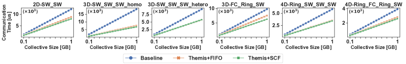
Figure 8. Total communication time of baseline, Themis+FIFO, and Themis+SCF for different size All-Reduces. Note that Themis+FIFO uses FIFO intra-dimension chunk scheduling, while Themis+SCF uses the smallest available chunks for intra-dimension chunk execution.

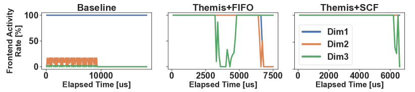
Figure 9. The average per-dimension activity rate for, Themis+FIFO, and Themis+Smallest-Chunk-First (SCF) for a 1GB All-Reduce size when running on 3D-SW_SW_SW_homo topology. A dimension is called to have activity if there is at least one chunk in that dimension for processing at any given point in time. Frontend activity rate is obtained by calculating the percentage of times each dimension has activity during a period of 100$\mu s$.

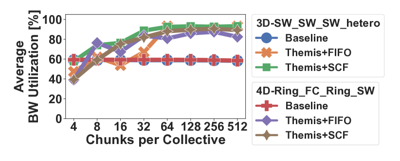
Figure 10. Sensitivity analysis that shows total BW utilization for a single 100MB All-Reduce when the number of chunks per collective varies from 4 to 512. The target topologies are 3D-SW_SW_SW_hetero and 4D-Ring_FC_Ring_SW.

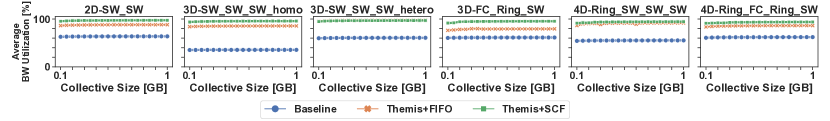
Figure 11. Average BW utilization of baseline, Themis+FIFO, and Themis+Smallest-Chunk-First (SCF) for different size All-Reduces.

Fig. 11 shows the average network utilization for variable sizes All-Reduce sizes. In general, as the collective size increases, its performance becomes more BW bound and the network latency component is minimized, leading to increased BW utilization. But the baseline scheduling cannot saturate the full BW as a result of the fundamental mismatch between different stage latencies of the hierarchical collective algorithms. On average, baseline, Themis+FIFO, and Themis+SCF can achieve 56.31%, 87.67%, and 95.14% of the network BW utilization, respectively. This indicates that Themis is an efficient method that can exploit and leverage almost all underutilized opportunities which exist in the baseline, leaving less room for further optimizations.

Next, we study the effect of chunk granularity on the performance of Themis. Fig. 10 shows the BW utilization for different number chunk granularities for baseline and Themis when running on 3D-SW_SW_SW_hetero and 4D-Ring_FC_Ring_SW topologies. Other topologies are not included due to space limitations. For the baseline, dim1 is the bottleneck (on both topologies) and the latency is mostly determined by the rate dim1 receives the chunks to process. Since dim1 is always the first dimension to receive the chunks in the baseline scheduling, changing the chunk granularity does not significantly affect its performance. However, increasing the number of chunks (decreasing chunk size) enables Themis to better balance the loads across the dimensions. When increasing the chunks from 4 to 512, BW utilization for Themis+SCF (Themis+FIFO) increases from 48.58% (43.13%) to 91.18% (87.81%) on average across the two topologies. In contrast, increasing the number of chunks per collective (reducing chunk size) might eventually reduce the individual chunk network operations to go below the max packet size on some network dimensions. This increases the header-to-packet ratio and hurts the network’s goodput.

We picked the default number of chunks to be 64 that achieve 95.14% BW utilization for the microbenchmark workload when averaging across all of our target topologies and collective sizes. This comes at the expense of increasing the total header-to-packet ratio by less than $0.5\%$ in the worst case (i.e., 100 MB AR), when compared to 1 chunk per collective for the microbenchmark workload.

As can be seen in Fig. 10, at some points, increasing chunks modestly reduces the BW utilization for Themis. This is mainly because of the starvation case discussed earlier. However, Themis+SCF shows stable behavior starting from 8 chunks on all of our tested topologies.

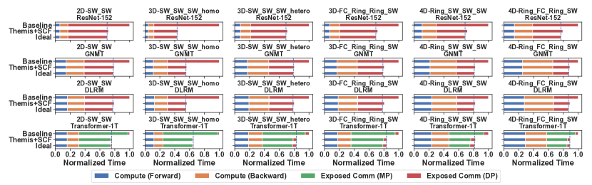
Figure 12. Training times for 3 iterations for ResNet-152, GNMT, DLRM, and Transformer-1T running on different topologies. Training iteration consists of a forward-pass followed by a back-propagation step. The total latency is decomposed to the compute times (across all layers), plus the total exposed communication latency. Compute times stem from computation during the forward pass (blue bar) or during the backpropagation (orange bar). Exposed communication may be due to the waiting for the data-parallel communications (red bar), or model-parallel communication (green bar), as explained in Sec. 5.2. For each workload, the latency of the baseline is normalized to 1.

6.2. Real Workload Results

In this section, we present real workload results to find the effect of Themis on the total end-to-end training iteration times which we break into total computation + exposed communication.. Here, we only use Themis+SCF configuration since it was shown to be the better approach in Sec. 6.1.

In our case and for the data-parallel partitioning, exposed communication occurs at the end of back-propagation, where NPUs communicate their locally computed weight gradients through All-Reduce, updating their model parameters before the next iteration starts.

Handling the model-parallel communication case is different in DLRM vs. Transformer-1T. For DLRM, its sparse features form a concurrent path with bottom-MLP layers, and therefore, its model-parallel communication (in terms of All-to-All collective operation) is performed in parallel with forward-pass, and back-propagation of bottom-MLPs. We only wait for the embedding communication operation (i.e. all-to-all) before entering the top-MLP layers in forward-pass, and after finishing the back-propagation to update the embedding. In the case of Transformer-1T, the output-activations/input-gradients of a (model-parallel) layer must be communicated (through AR or AG, depending on the layer type in Transformer) during forward-pass/back-propagation before processing the next layer. Fig. 12 shows the training iteration times that are decomposed into total compute time and total exposed communication time.

For training, back-propagation computation usually takes longer since it needs to compute for both weight gradients and input gradients, compared to the forward-pass that only involves forward computation. However, this is not the case for Transformer-1T since it consists of forward-in-back-propagation steps, as a result of ZeRO optimizer, that is counted towards forward-pass in Fig. 12.

As Fig. 12 shows, ResNet-152 and GNMT only experience data-parallel exposed communication since they are distributed in pure data-parallel. An interesting point is about DLRM where it has a hybrid (data+model parallel as explained in Sec. 5.2) parallelism, but only the data-parallel communication is counted towards exposed communication. This is because model-parallel communication (All-To-All) is overlapped with the forward-pass, back-propagation operations of bottom-MLP layers. In Transformer-1T the model-parallel communication is the dominant factor. Also, note that the data-parallel communication of Transformer-1T uses only the last network dimension in all of the topologies. This indicates that there is only one scheduling possible for data-parallel communication of Transformer-1T, meaning that baseline and Themis have the same performance for this portion of the exposed communication. When averaging across all topologies and workloads, applying Themis reduces the exposed communication time by 1.65$\times$. The speedup is close to the Ideal system which reduces the exposed communication time by 1.72$\times$, on average.

Such reduction in exposed communication leads to a reduction in overall training time as well. However, the overall training iteration benefit follows Amdahl’s law (Amdahl, 1967) and depends on the current ratio between the exposed communication and total computation. When averaging across all topologies, Themis reduces the training iteration time by 1.49$\times$ (2.25$\times$ max), 1.30$\times$ (1.78$\times$ max), 1.30$\times$ (1.77$\times$ max), and 1.25$\times$ (1.53$\times$ max) for ResNet-152, GNMT, DLRM, and Transformer-1T, respectively. On the other hand, the Ideal system achieves training iteration speed-up of 1.54$\times$, 1.32$\times$, 1.33$\times$, and 1.26$\times$ for ResNet-152, GNMT, DLRM, and Transformer-1T, respectively. Overall, we find Themis is close to the ideal system, leaving little opportunity for further optimization.

6.3. Insights for Future System Design

Throughout this paper, we showed how Themis can drive the BW of all network dimensions. This raises the question that how architects and system engineers should distribute the network BW across different network dimensions in the first place and whether some design points should be prohibited since even Themis cannot help. Consider any two dimensions dimK and dimL of the network, where K<L and $P_{I}$ to be the network size in dimI. In this section, we describe three different scenarios for BW distribution, depending on the BW provision for dimL:

Just Enough BW Scenario. Here, the baseline (and Themis) scheduling algorithm can fully utilize the network. As explained in Sec. 3, the BW distribution should be:

$$\text{BW(dimK)}=P_{K}\times P_{K+1}\times....\times P_{L-1}\times\text{BW(dimL)}$$

In this case, the chunk size ratio is proportional to the BW ratio of the two dimensions. Hence, the baseline algorithm is sufficient to utilize both dimensions.

OverProvisioned BW Scenario.

$$\text{BW(dimK)}<P_{K}\times P_{K+1}\times....\times P_{L-1}\times\text{BW(dimL)}$$

As explained in Sec. 3, this is the case where the baseline can not utilize the full BW of dimL. While Themis redistributes the loads that result in full utilization of both dimensions.

UnderProvisioned BW Scenario. In this case there may be no scheduling algorithm that can fully drive both dimensions:

$$\text{BW(dimK)}>P_{K}\times P_{K+1}\times....\times P_{L-1}\times\text{BW(dimL)}$$

In such BW distribution and with baseline scheduling, dimK is underutilized while it has $P_{K}\times P_{K+1}\times....\times P_{L-1}$ more loads, compared to dimL (dimL has underprovisioned BW).

To fully utilize both dimensions, any redistribution of chunks should increase the load of dimK compared to dimL. However, this only can happen if dimK has overprovisioned BW compared to some other dimension and this might not always be the case. For example, in a simple 2-dimensional network case where K=1, L=2, there is no scheduling that can fully utilize both dimensions, since the baseline scheduling already puts the highest load on dimK, and any other scheduling increases the load gap between dimK and dimL (rather than reducing it). Thus, such design points should be prohibited.

7. Related Works

HPC Platforms. Collective communication algorithms are vastly studied in the context of High Performance Computing (HPC) workloads using the MPI communication interface (MPI, 2015). Many different implementations of MPI interface are proposed in (Thakur et al., 2005; Chan et al., 2007; Pjesivac-Grbovic et al., 2005), as well as topology-aware algorithms (Barnett et al., 1993; Bokhari and Berryman, 1992; Zhu et al., 2009), and efficient collective execution on shared-memory processor clusters (Sistare et al., 1999; Tipparaju et al., 2003). Nonetheless, these CPU-based collective algorithms either assume BW-symmetric topology or apply hierarchical algorithms with a fixed schedule. Moreover, collectives in HPC are usually small (few KB-MB) unlike DL (10s of MB-GB) where they lie in the critical path (Klenk et al., 2020).

DL Training Platforms (1-dimensional). Recently, collective communications are revisited for direct NPU-to-NPU communications for distributed DNN workloads. SCCL (Cai et al., 2021) provides topology-aware pareto-optimal collectives for a given topology. EFLOPS (Dong et al., 2020) proposes a BiGraph topology with optimized HDRM collective algorithm. However, these works are based on BW-symmetric and 1-dimensional networks only.

DL Training Platforms (Multi-dimensional). In addition, collective communication libraries such as (ncc, 2017; Intel, 2020; Cowan et al., 2022) provide a suite of collective algorithms optimized for various topology and collective sizes. Authors in (Wang et al., 2020; Luo et al., 2020; Cho et al., 2019) take into account the physical topology hierarchies to perform localized reduction/aggregation per each network hierarchy. Blink (Wang et al., 2020) is a framework to generate efficient collective algorithms based on the underlying network resources using the concept of packing spanning trees. PLink (Luo et al., 2020) is a collective scheme that aims to cope with the heterogeneous network and variable performance of public cloud platforms. It creates a logical 2-dimensional network based on the distance proximity of VMs, and then applies a hierarchical collective algorithm to optimize for heterogeneous cloud network, and dynamically changes the collective algorithm within each (logical) network dimension to adapt to the performance variability due to other interfering workloads. However, all of these works perform hierarchical collectives with the static schedule of chunk operations across different network dimensions, which is not efficient for the next-gen platforms as discussed in this paper.

In contrast, Themis is the first method that proposes a dynamic chunk scheduling for maximum BW utilization. Themis is also orthogonal to all previous hierarchical collective methods, meaning that it can leverage any proposed collective algorithm for each dimension, while only changing the schedules of each individual chunk.

8. Conclusion

In this paper, we identified that hierarchical multi-stage collective algorithms fail to saturate the network BW of next-gen platforms due to different pipeline stage latencies induced by different chunk sizes and network characteristics in each network dimension. We proposed Themis as a solution to improve the BW utilization by dynamically scheduling the chunks to balance the loads across different network dimensions.

Themis improves the end-to-end training iteration performance of real workloads, such as ResNet-152, GNMT, DLRM, and Transformer-1T, by 1.49$\times$ (2.25$\times$ max), 1.30$\times$ (1.78$\times$ max), 1.30$\times$ (1.77$\times$ max), and 1.25$\times$ (1.53$\times$ max), respectively.

- (1)
- Inf (2008) 2008. Introduction to InfiniBand™. https://network.nvidia.com/related-docs/whitepapers/IB_Intro_WP_190.pdf.
- MPI (2015) 2015. MPI: A Message-Passing Interface Standard. https://www.mpi-forum.org/docs/mpi-3.1/mpi31-report.pdf.
- Gra (2016) 2016. Graphcore. https://www.graphcore.ai/.
- int (2016) 2016. Habana. https://habana.ai.
- ncc (2017) 2017. NVIDIA Collective Communication Library (NCCL). https://developer.nvidia.com/nccl
- goo (2018) 2018. Cloud TPU. https://cloud.google.com/tpu.
- Hab (2019) 2019. Gaudi Training Platfrom White Paper. https://habana.ai/wp-content/uploads/2019/06/Habana-Gaudi-Training-Platform-whitepaper.pdf.
- Cis (2019) 2019. Introduction to High Bandwidth and Low Latency Network Design with 400GE. https://www.ciscolive.com/c/dam/r/ciscolive/us/docs/2019/pdf/BRKDCN-2213.pdf.
- dgx (2019) 2019. NVIDIA DGX-2. https://www.nvidia.com/en-us/data-center/dgx-2/
- Int (2019) 2019. The First Xe-HPC Deployment: Aurora, with Xe Link. https://www.anandtech.com/show/15188/analyzing-intels-discrete-xe-hpc-graphics-disclosure-ponte-vecchio/5.
- Ast (2020) 2020. ASTRA-SIM: Enabling SW/HW Co-Design Exploration for Distributed DL Training Platforms. https://github.com/astra-sim/astra-sim.git.
- Mel (2020) 2020. Mellanox SHARP. https://docs.mellanox.com/display/sharpv214.
- A10 (2020) 2020. NVIDIA A100 Tensor Core GPU. https://www.nvidia.com/en-us/data-center/a100/.
- AMD (2021) 2021. AMD Infinity Architecture. https://www.amd.com/en/technologies/infinity-architecture.
- Amd (2021) 2021. AMD Instinct™ MI250X Accelerator. amd.com/en/products/server-accelerators/instinct-mi250x.
- NIC (2021) 2021. ConnectX SmartNICs. https://www.nvidia.com/en-in/networking/ethernet-adapters/.
- fb_(2021) 2021. Fully Sharded Data Parallel: faster AI training with fewer GPUs. https://engineering.fb.com/2021/07/15/open-source/fsdp.
- Tra (2021) 2021. Google Open-Sources Trillion-Parameter AI Language Model Switch Transformer. https://www.infoq.com/news/2021/02/google-trillion-parameter-ai/.
- NVI (2021) 2021. NVIDIA DGX SuperPOD: Instant Infrastructure for AI Leadership. https://resources.nvidia.com/en-us-auto-datacenter/nvpod-superpod-wp-09.
- Int (2022) 2022. Intel Ponte Vecchio. https://www.nextplatform.com/2021/08/24/intels-ponte-vecchio-gpu-better-not-be-a-bridge-too-far/.
- Nvi (2022) 2022. NVIDIA H100 Tensor Core GPU. https://www.nvidia.com/en-us/data-center/h100/.
- NVL (2022) 2022. NVLink AND NVSwitch. https://www.nvidia.com/en-us/data-center/nvlink/.
- Amdahl (1967) Gene M. Amdahl. 1967. Validity of the Single Processor Approach to Achieving Large Scale Computing Capabilities. In April 18-20, 1967, Spring Joint Computer Conference (AFIPS). 483–485. https://doi.org/10.1145/1465482.1465560
- Amodei and Hernandez (2018) Dario Amodei and Danny Hernandez. 2018. AI and Compute. https://openai.com/blog/ai-and-compute/
- Arunkumar et al. (2017) Akhil Arunkumar, Evgeny Bolotin, Benjamin Cho, Ugljesa Milic, Eiman Ebrahimi, Oreste Villa, Aamer Jaleel, Carole-Jean Wu, and David Nellans. 2017. MCM-GPU: Multi-Chip-Module GPUs for Continued Performance Scalability. In 44th Annual International Symposium on Computer Architecture (ISCA). 320–332. https://doi.org/10.1145/3079856.3080231
- Barnett et al. (1993) M. Barnett, R. Littlefield, D.G. Payne, and R. van de Geijn. 1993. Global combine on mesh architectures with wormhole routing. In 7th International Parallel Processing Symposium (IPPS). 156–162. https://doi.org/10.1109/IPPS.1993.262873
- Bokhari and Berryman (1992) Shahid H. Bokhari and Harry. Berryman. 1992. Complete exchange on a circuit switched mesh. In 1992 Scalable High Performance Computing Conference (SHPCC). 300–306. https://doi.org/10.1109/SHPCC.1992.232628
- Cai et al. (2021) Zixian Cai, Zhengyang Liu, Saeed Maleki, Madanlal Musuvathi, Todd Mytkowicz, Jacob Nelson, and Olli Saarikivi. 2021. Synthesizing Optimal Collective Algorithms. In 26th ACM SIGPLAN Symposium on Principles and Practice of Parallel Programming (PPoPP). 62–75. https://doi.org/10.1145/3437801.3441620
- Chan et al. (2007) Ernie Chan, Marcel Heimlich, Avi Purkayastha, and Robert van de Geijn. 2007. Collective Communication: Theory, Practice, and Experience: Research Articles. Concurrency and Computation: Practice and Experience 19, 13 (Sep. 2007), 1749–1783.
- Chan et al. (2006) Ernie Chan, Robert van de Geijn, William Gropp, and Rajeev Thakur. 2006. Collective Communication on Architectures That Support Simultaneous Communication over Multiple Links. In 11th ACM SIGPLAN Symposium on Principles and Practice of Parallel Programming (PPoPP). 2–11. https://doi.org/10.1145/1122971.1122975
- Cho et al. (2019) M. Cho, U. Finkler, M. Serrano, D. Kung, and H. Hunter. 2019. BlueConnect: Decomposing all-reduce for deep learning on heterogeneous network hierarchy. IBM Journal of Research and Development 63, 6 (Oct. 2019), 1:1–11. https://doi.org/10.1147/JRD.2019.2947013
- Cowan et al. (2022) Meghan Cowan, Saeed Maleki, Madanlal Musuvathi, Olli Saarikivi, and Yifan Xiong. 2022. GC3: An Optimizing Compiler for GPU Collective Communication. arXiv:2201.11840 [cs.DC]
- De Sensi et al. (2021) Daniele De Sensi, Salvatore Di Girolamo, Saleh Ashkboos, Shigang Li, and Torsten Hoefler. 2021. Flare: Flexible in-Network Allreduce. In International Conference for High Performance Computing, Networking, Storage and Analysis (SC). 1–16. https://doi.org/10.1145/3458817.3476178
- Dong et al. (2020) Jianbo Dong, Zheng Cao, Tao Zhang, Jianxi Ye, Shaochuang Wang, Fei Feng, Li Zhao, Xiaoyong Liu, Liuyihan Song, Liwei Peng, Yiqun Guo, Xiaowei Jiang, Lingbo Tang, Yin Du, Yingya Zhang, Pan Pan, and Yuan Xie. 2020. EFLOPS: Algorithm and System Co-Design for a High Performance Distributed Training Platform. In 2020 IEEE International Symposium on High Performance Computer Architecture (HPCA). 610–622. https://doi.org/10.1109/HPCA47549.2020.00056
- Ethernet Technology Consortium (2020) Ethernet Technology Consortium. 2020. 800G Specification. https://ethernettechnologyconsortium.org/wp-content/uploads/2020/03/800G-Specification_r1.0.pdf.
- Harlap et al. (2018) Aaron Harlap, Deepak Narayanan, Amar Phanishayee, Vivek Seshadri, Nikhil Devanur, Greg Ganger, and Phil Gibbons. 2018. PipeDream: Fast and Efficient Pipeline Parallel DNN Training. arXiv:1806.03377 [cs.DC]
- He et al. (2015) Kaiming He, Xiangyu Zhang, Shaoqing Ren, and Jian Sun. 2015. Deep Residual Learning for Image Recognition. arXiv:1512.03385 [cs.CV]
- Huang et al. (2019) Yanping Huang, Youlong Cheng, Ankur Bapna, Orhan Firat, Mia Xu Chen, Dehao Chen, HyoukJoong Lee, Jiquan Ngiam, Quoc V. Le, Yonghui Wu, and Zhifeng Chen. 2019. GPipe: Efficient Training of Giant Neural Networks using Pipeline Parallelism. arXiv:1811.06965 [cs.CV]
- Intel (2020) Intel. 2020. Intel oneAPI Collective Communications Library. https://software.intel.com/content/www/us/en/develop/tools/oneapi/components/oneccl.html
- Jerger et al. (2017) Natalie Enright Jerger, Tushar Krishna, and Li-Shiuan Peh. 2017. On-chip networks. Synthesis Lectures on Computer Architecture 12, 3 (2017), 1–210.
- Jia et al. (2018) Xianyan Jia, Shutao Song, Wei He, Yangzihao Wang, Haidong Rong, Feihu Zhou, Liqiang Xie, Zhenyu Guo, Yuanzhou Yang, Liwei Yu, Tiegang Chen, Guangxiao Hu, Shaohuai Shi, and Xiaowen Chu. 2018. Highly Scalable Deep Learning Training System with Mixed-Precision: Training ImageNet in Four Minutes. arXiv:1807.11205 [cs.LG]
- Kazemivash and Calhoun (2020) Behnam Kazemivash and Vince D. Calhoun. 2020. BPARC: A novel spatio-temporal (4D) data-driven brain parcellation scheme based on deep residual networks. In IEEE 20th International Conference on Bioinformatics and Bioengineering (BIBE). 1071–1076. https://doi.org/10.1109/BIBE50027.2020.00181
- Kazemivash and Calhoun (2022) Behnam Kazemivash and Vince D. Calhoun. 2022. A novel 5D brain parcellation approach based on spatio-temporal encoding of resting fMRI data from deep residual learning. Journal of Neuroscience Methods 369 (2022), 109478. https://doi.org/10.1016/j.jneumeth.2022.109478
- Klenk et al. (2020) Benjamin Klenk, Nan Jiang, Greg Thorson, and Larry Dennison. 2020. An In-Network Architecture for Accelerating Shared-Memory Multiprocessor Collectives. In 47th Annual International Symposium on Computer Architecture (ISCA). 996–1009. https://doi.org/10.1109/ISCA45697.2020.00085
- Li et al. (2019b) Ang Li, Shuaiwen Leon Song, Jieyang Chen, Jiajia Li, Xu Liu, Nathan R. Tallent, and Kevin J. Barker. 2019b. Evaluating Modern GPU Interconnect: PCIe, NVLink, NV-SLI, NVSwitch and GPUDirect. arXiv:1903.04611 [cs.AR]
- Li et al. (2019a) Youjie Li, Iou-Jen Liu, Yifan Yuan, Deming Chen, Alexander Schwing, and Jian Huang. 2019a. Accelerating Distributed Reinforcement Learning with In-Switch Computing. In 46th International Symposium on Computer Architecture (ISCA). 279–291. https://doi.org/10.1145/3307650.3322259
- Luo et al. (2020) Liang Luo, Peter West, Jacob Nelson, Arvind Krishnamurthy, and Luis Ceze. 2020. PLink: Discovering and Exploiting Locality for Accelerated Distributed Training on the public Cloud. In 2022 Machine Learning and Systems (MLSys). 82–97. https://proceedings.mlsys.org/paper/2020/file/182be0c5cdcd5072bb1864cdee4d3d6e-Paper.pdf
- Mudigere et al. (2021) Dheevatsa Mudigere, Yuchen Hao, Jianyu Huang, Zhihao Jia, Andrew Tulloch, Srinivas Sridharan, Xing Liu, Mustafa Ozdal, Jade Nie, Jongsoo Park, Liang Luo, Jie Amy Yang, Leon Gao, Dmytro Ivchenko, Aarti Basant, Yuxi Hu, Jiyan Yang, Ehsan K. Ardestani, Xiaodong Wang, Rakesh Komuravelli, Ching-Hsiang Chu, Serhat Yilmaz, Huayu Li, Jiyuan Qian, Zhuobo Feng, Yinbin Ma, Junjie Yang, Ellie Wen, Hong Li, Lin Yang, Chonglin Sun, Whitney Zhao, Dimitry Melts, Krishna Dhulipala, KR Kishore, Tyler Graf, Assaf Eisenman, Kiran Kumar Matam, Adi Gangidi, Guoqiang Jerry Chen, Manoj Krishnan, Avinash Nayak, Krishnakumar Nair, Bharath Muthiah, Mahmoud khorashadi, Pallab Bhattacharya, Petr Lapukhov, Maxim Naumov, Ajit Mathews, Lin Qiao, Mikhail Smelyanskiy, Bill Jia, and Vijay Rao. 2021. Software-Hardware Co-design for Fast and Scalable Training of Deep Learning Recommendation Models. arXiv:2104.05158 [cs.DC]
- Naumov et al. (2019) Maxim Naumov, Dheevatsa Mudigere, Hao-Jun Michael Shi, Jianyu Huang, Narayanan Sundaraman, Jongsoo Park, Xiaodong Wang, Udit Gupta, Carole-Jean Wu, Alisson G. Azzolini, Dmytro Dzhulgakov, Andrey Mallevich, Ilia Cherniavskii, Yinghai Lu, Raghuraman Krishnamoorthi, Ansha Yu, Volodymyr Kondratenko, Stephanie Pereira, Xianjie Chen, Wenlin Chen, Vijay Rao, Bill Jia, Liang Xiong, and Misha Smelyanskiy. 2019. Deep Learning Recommendation Model for Personalization and Recommendation Systems. arXiv:1906.00091 [cs.IR]
- Patarasuk and Yuan (2009) Pitch Patarasuk and Xin Yuan. 2009. Bandwidth Optimal All-reduce Algorithms for Clusters of Workstations. Parallel and Distributed Computing 69, 2 (Feb. 2009), 117–124. https://doi.org/10.1016/j.jpdc.2008.09.002
- Pjesivac-Grbovic et al. (2005) Jelena Pjesivac-Grbovic, Thara Angskun, George Bosilca, Graham E. Fagg, Edgar Gabriel, and Jack J. Dongarra. 2005. Performance analysis of MPI collective operations. In 19th IEEE International Parallel and Distributed Processing Symposium (IPDPS). 1–8. https://doi.org/10.1109/IPDPS.2005.335
- Rajbhandari et al. (2020) Samyam Rajbhandari, Jeff Rasley, Olatunji Ruwase, and Yuxiong He. 2020. ZeRO: Memory Optimizations Toward Training Trillion Parameter Models. arXiv:1910.02054 [cs.LG]
- Rashidi et al. (2021) Saeed Rashidi, Matthew Denton, Srinivas Sridharan, Sudarshan Srinivasan, Amoghavarsha Suresh, Jade Nie, and Tushar Krishna. 2021. Enabling Compute-Communication Overlap in Distributed Deep Learning Training Platforms. In 2021 ACM/IEEE 48th Annual International Symposium on Computer Architecture (ISCA). 540–553. https://doi.org/10.1109/ISCA52012.2021.00049
- Rashidi et al. (2020a) Saeed Rashidi, Pallavi Shurpali, Srinivas Sridharan, Naader Hassani, Dheevatsa Mudigere, Krishnakumar Nair, Misha Smelyanski, and Tushar Krishna. 2020a. Scalable Distributed Training of Recommendation Models: An ASTRA-SIM + NS3 case-study with TCP/IP transport. In 2020 IEEE Symposium on High-Performance Interconnects (HOTI). 33–42. https://doi.org/10.1109/HOTI51249.2020.00020
- Rashidi et al. (2020b) Saeed Rashidi, Srinivas Sridharan, Sudarshan Srinivasan, and Tushar Krishna. 2020b. ASTRA-SIM: Enabling SW/HW Co-Design Exploration for Distributed DL Training Platforms. In 2020 IEEE International Symposium on Performance Analysis of Systems and Software (ISPASS). 81–92. https://doi.org/10.1109/ISPASS48437.2020.00018
- Shah et al. (2021) Aashaka Shah, Vijay Chidambaram, Meghan Cowan, Saeed Maleki, Madan Musuvathi, Todd Mytkowicz, Jacob Nelson, Olli Saarikivi, and Rachee Singh. 2021. Synthesizing Collective Communication Algorithms for Heterogeneous Networks with TACCL. arXiv:2111.04867 [cs.DC]
- Shao et al. (2019) Yakun Sophia Shao, Jason Clemons, Rangharajan Venkatesan, Brian Zimmer, Matthew Fojtik, Nan Jiang, Ben Keller, Alicia Klinefelter, Nathaniel Pinckney, Priyanka Raina, Stephen G. Tell, Yanqing Zhang, William J. Dally, Joel Emer, C. Thomas Gray, Brucek Khailany, and Stephen W. Keckler. 2019. Simba: Scaling Deep-Learning Inference with Multi-Chip-Module-Based Architecture. In 52nd Annual IEEE/ACM International Symposium on Microarchitecture (MICRO). 14–27. https://doi.org/10.1145/3352460.3358302
- Sistare et al. (1999) Steve Sistare, Rolf Vandevaart, and Eugene Loh. 1999. Optimization of MPI Collectives on Clusters of Large-Scale SMP’ s. In 1999 ACM/IEEE Conference on Supercomputing (SC). 23–23. https://doi.org/10.1109/SC.1999.10010
- Thakur et al. (2005) Rajeev Thakur, Rolf Rabenseifner, and William Gropp. 2005. Optimization of Collective Communication Operations in MPICH. International Journal of High Performance Computing Applications 19, 1 (Feb. 2005), 49–66. https://doi.org/10.1177/1094342005051521
- Thangakrishnan et al. (2020) Indu Thangakrishnan, Derya Cavdar, Can Karakus, Piyush Ghai, Yauheni Selivonchyk, and Cory Pruce. 2020. Herring: Rethinking the Parameter Server at Scale for the Cloud. In International Conference for High Performance Computing, Networking, Storage and Analysis (SC). 1–13. https://doi.org/10.1109/SC41405.2020.00048
- Tipparaju et al. (2003) Vinod Tipparaju, Jarek Nieplocha, and Dhabaleswar Panda. 2003. Fast collective operations using shared and remote memory access protocols on clusters. In 2003 International Parallel and Distributed Processing Symposium (IPDPS). 1–10. https://doi.org/10.1109/IPDPS.2003.1213188
- Vaswani et al. (2017) Ashish Vaswani, Noam Shazeer, Niki Parmar, Jakob Uszkoreit, Llion Jones, Aidan N. Gomez, Lukasz Kaiser, and Illia Polosukhin. 2017. Attention Is All You Need. arXiv:1706.03762 [cs.CL]
- Wang et al. (2020) Guanhua Wang, Shivaram Venkataraman, Amar Phanishayee, Nikhil Devanur, Jorgen Thelin, and Ion Stoica. 2020. Blink: Fast and Generic Collectives for Distributed ML. In 2020 Machine Learning and Systems (MLSys). 172–186. https://proceedings.mlsys.org/paper/2020/file/43ec517d68b6edd3015b3edc9a11367b-Paper.pdf
- Wu et al. (2016) Yonghui Wu, Mike Schuster, Zhifeng Chen, Quoc V. Le, Mohammad Norouzi, Wolfgang Macherey, Maxim Krikun, Yuan Cao, Qin Gao, Klaus Macherey, Jeff Klingner, Apurva Shah, Melvin Johnson, Xiaobing Liu, Lukasz Kaiser, Stephan Gouws, Yoshikiyo Kato, Taku Kudo, Hideto Kazawa, Keith Stevens, George Kurian, Nishant Patil, Wei Wang, Cliff Young, Jason Smith, Jason Riesa, Alex Rudnick, Oriol Vinyals, Greg Corrado, Macduff Hughes, and Jeffrey Dean. 2016. Google’s Neural Machine Translation System: Bridging the Gap between Human and Machine Translation. arXiv:1609.08144 [cs.CL]
- Yasaman Ghadar and Tim Williams (2020) Yasaman Ghadar and Tim Williams. 2020. An Overview of Aurora, Argonne’s Upcoming Exascale System. https://ecpannualmeeting.com/assets/overview/sessions/Aurora-Public-FULL-talk-Feb-4-2020_for_posting_c.pdf
- Zhu et al. (2009) Hao Zhu, David Goodell, William Gropp, and Rajeev Thakur. 2009. Hierarchical Collectives in MPICH2. In 16th European PVM/MPI Users’ Group Meeting on Recent Advances in Parallel Virtual Machine and Message Passing Interface (EuroPVM/MPI). 325–326. https://doi.org/10.1007/978-3-642-03770-2_41