A Novel Quantum Calculus-based Complex Least Mean Square Algorithm ($q$-CLMS)

Abstract

In this research, a novel adaptive filtering algorithm is proposed for complex domain signal processing. The proposed algorithm is based on Wirtinger calculus and is called as q-Complex Least Mean Square (q-CLMS) algorithm. The proposed algorithm could be considered as an extension of the $q$-LMS algorithm for the complex domain. Transient and steady-state analyses of the proposed $q$-CLMS algorithm are performed and exact analytical expressions for mean analysis, mean square error (MSE), excess mean square error (EMSE), mean square deviation (MSD) and misadjustment are presented. Extensive experiments have been conducted and a good match between the simulation results and theoretical findings is reported. The proposed $q$-CLMS algorithm is also explored for whitening applications with satisfactory performance. A modification of the proposed $q$-CLMS algorithm called Enhanced $q$-CLMS (E$q$-CLMS) is also proposed. The E$q$-CLMS algorithm eliminates the need for a pre-coded value of the $q$-parameter thereby automatically adapting to the best value. Extensive experiments are performed on system identification and channel equalization tasks and the proposed algorithm is shown to outperform several benchmark and state-of-the-art approaches namely Complex Least Mean Square (CLMS), Normalized Complex Least Mean Square (NCLMS), Variable Step Size Complex Least Mean Square (VSS-CLMS), Complex FLMS (CFLMS) and Fractional-ordered-CLMS (FoCLMS) algorithms.

1 Introduction

Adaptive algorithms have been successfully applied in a number of signal processing applications such as channel equalization, noise cancellation, system identification and optimization, etc NCLMS ; AI3 ; VanKien2021 . Adaptive learning frameworks have also been traditionally used for regression, classification Ibrokhimov2021 and dimensionality reduction Wu2021 ; Chen2021 encompassing several applications such as image segmentation Ding2021 , quality enhancement Li2021 , etc.

The Least Mean Square (LMS) method is considered to be a cornerstone approach with several merits and is one of the most widely used adaptive algorithms. Because the LMS is dependent on the eigenvalue spread of the input correlation matrix, it suffers from slow convergence. Several adaptive strategies, such as normalized LMS (NLMS), computed adaptive learning rates, a chaotic teaching-learning based optimization, variable power fractional LMS algorithm, and variable step-size LMS algorithm, have been presented in the literature to address this issue, NLMS ; AI1 ; VPFLMS ; RVPFLMS ; RVSSFLMS ; VSS .

Recently, an interesting variant of the traditional LMS algorithm, called the q-LMS qLMS , has been proposed. The q-LMS algorithm computes the derivative of the cost function using secant rather than tangent function as it utilizes the notion of $q$-gradient qLMS . The method is shown to achieve a higher convergence rate, compared to the conventional LMS, while maintaining competitive performance. In 8955461 ; qNLMS ; mishra2021q ; hussain2021q ; EqLMS ; sadiq2020q , adaptive techniques are further proposed for the $q$ parameter. The q-LMS algorithm also been successfully implemented for system identification, unconstrained optimization, neural networks and the design of whitening filters tasks.

Typically, adaptive filters are used with real-valued signals and systems. For signals with intensity and direction components, complex domain provides an efficient framework direction . As adaptive algorithms requires the minimization of a cost function through differentiation, wirtinger calculus is used for the evaluation of a cost function in complex domain. In a number of fields such as beamforming, object detection, bio-medicine and communications, complex modeling of signals and systems is required khan2020adaptive ; radar ; biomed . A number of applications of Wirtinger calculus can be found in areas such as high performance distribution networks, complex-valued neural networks and complex kernel LMSpowerflow ; CVNN ; CKLMS . The analysis of such systems is not straightforward. Simplified approaches, such as the processing of the imaginary and real parts separately, tend to limit the usefulness of the complex domain. The cornerstone work in this regard is the CLMS (Complex Least Mean Square) CLMS with the weight update equation:

$$\mathbf{w}(n+1)=\mathbf{w}(n)+2\mu\mathbf{x}(n)e^{*}(n).$$ (1)

where $\mu$ is the convergence factor, $e^{*}(n)$ is the conjugate of the error, and $\mathbf{w}(n)$ and $\mathbf{w}(n+1)$ are the current and updated weights, respectively. The CLMS algorithm has been applied in various fields, such as adaptive prediction, system identification and complex dual-channel estimation. There are some existing works in the literature to improve the CLMS algorithm and various variants have been proposed LMS9 ; LMS11 ; FCLMS ; RNACLMS ; Shah2017 ; Ahmad2021 . In this study, we propose a quantum variant of the complex least mean square by utilizing the novel q-wirtinger calculus based q-steepest decent method. To the best of our knowledge, this is for the first time where a quantum calculus-based approach has been applied to design an adaptive learning method for the complex domain signal processing applications. The proposed algorithm is called as the $q$-CLMS ($q$-Complex Least Mean Square) algorithm. Major contributions of the proposed research are as follows:

• A novel q-calculus-based adaptive filtering algorithm is proposed for the complex domain (section 3). In particular, the notion of the $q$-LMS is extended to the complex domain using the Wirtinger calculus. ASP .

• Extensive theoretical analysis of the proposed q-CLMS algorithm, consisting of the mean and the mean-square error convergence, is performed. Learning curves for Excess Mean Square Error (EMSE), Mean Square Deviation (MSD), and misadjustment is also derived.

• The proposed $q$-CLMS is further improved by making the $q$-parameter time-varying (section 4). This modified approach eliminates the need for a pre-coded value of the $q$-parameter by automatically adapting to the best value. The modified approach is called Enhanced q-CLMS (Eq-CLMS).

• For the system identification task, compact analytical forms have been derived and validated through the simulation results (sub-section 6.2).

• For the selection of $q$-parameter, the q-gradient is applied in such a manner as to make the LMS filter perform as a whitening filter.

• Extensive comparative analysis has been carried out for the proposed algorithm where results are compared to several state-of-the-art approaches namely the complex LMS (CLMS), normalized CLMS (NCLMS) and variable step-size CLMS (VSS-CLMS). The experiments clearly show the efficacy of the proposed approach.

• To show the efficacy of the proposed method, channel equalization task has been addressed and the comparison has been made with the fractional variants of the LMS namely, CFLMS Shah2017 and FoCLMS Ahmad2021 .

The rest of the paper is composed as follows: In Section 2, q-calculus and the $q$-steepest descent algorithm are explained. The proposed q-CLMS algorithm is discussed with detailed analysis in Section 3. The proposed $q$-CLMS algorithm is modified to an adaptive version i.e., E$q$-CLMS in Section 4. An interesting application of the proposed methodology namely the whitening filter is discussed in Section 5 followed by extensive experiments and results in Section 6. The paper is finally concluded in Section 7.

2 The Proposed q-Wirtinger calculus

Quantum calculus is often specified as the calculus with no limits qbook1 . It has been applied in numerous fields and a collection of new outcomes can be found in qbook2 ; qbook3 ; qbook4 .

The differential of a function in quantum calculus is given as kac2001quantum :

$$d_{q}(f(x))=f(qx)-f(x).$$ (2)

Consequently, the derivative of a function is defined as

$$D_{q}(f(x))=\frac{d_{q}(f(x))}{d_{q}(x)}=\frac{f(qx)-f(x)}{(q-1)x}.$$ (3)

The formula takes the form of the standard derivative as q approaches 1. For the function $x^{n}$, the q-derivative is given as:

$$D_{q,x}x^{n}=\begin{cases}\displaystyle\frac{q^{n}-1}{q-1}x^{n-1},&q\neq 1,\\ \displaystyle nx^{n-1},&q=1.\end{cases}$$ (4)

The q-gradient of a function $f(\mathbf{x})$, for $n$ number of variables, $\mathbf{x}(n)=[{x}_{1}(n),{x}_{2}(n),\dots x_{M}(n)]^{\intercal}$, is defined as nthpower

$$\nabla_{\mathbf{q,x}}f(\mathbf{x})\triangleq[D_{q1,x1}f(\mathbf{x}),D_{q2,x2}f(\mathbf{x}),...D_{qn,xn}f(\mathbf{x})]^{\intercal},$$ (5)

Alternatively, $\nabla_{\mathbf{q,x}}f(\mathbf{x})$ can also be written as:

$$\nabla_{\mathbf{q}}f(\mathbf{x})(\mathbf{x})\triangleq[D_{q1}f(\mathbf{x})(x_{1}),D_{q2}f(\mathbf{x})(x_{2}),...D_{q}f(\mathbf{x})(x_{n})]^{\intercal},$$ (6)

where $\mathbf{q}(n)=[{q}_{1}(n),{q}_{2}(n),\dots q_{M}(n)]^{\intercal}$.
q-calculus is a well-established field with well-defined rules qbook1 . For ordinary derivatives, the chain rule is as follows:
Let $g(x)=cx^{k}$. Then

$$D_{q}f(g(x))=D_{q}^{k}(f)(g(x))D_{q}(g)(x).$$ (7)

The gradient descent methodology is employed in a number of adaptive algorithms, and the $q$-calculus has been employed to develop the $q$-gradient descent for real systems by calculating the secant of the cost-function. (Section 1)

2.1 q-Steepest Descent

The Weight-update equation of the conventional steepest descent algorithm is given as:

$$\mathbf{w}(n+1)=\mathbf{w}(n)-\mu\nabla_{\mathbf{w}}J(\mathbf{w}).$$ (8)

where $\mu$ denotes the step size, $\mathbf{w}(n)$ and $\mathbf{w}(n+1)$ denote the current and updated weights, and $J(\mathbf{w})$ denotes the steepest descent algorithm’s cost function, which is given as:

$$J(\mathbf{w})=e^{2}(n)$$ (9)

The estimation error, denoted by the symbol $e(n)$, is defined as the difference between the desired and the output signal. It is written as follows:

$$e(n)=d(n)-y(n)$$ (10)

Replacing the conventional gradient in Eq.(8) by the $q$ derivative:

$$\mathbf{w}(n+1)=\mathbf{w}(n)-\mu\nabla_{\mathbf{q,w}}J(\mathbf{w}).$$ (11)

Now, by using Eqs.(4) and (5), the $\nabla_{\mathbf{q,w}}J(\mathbf{w})$ is calculated as qLMS

$$\nabla_{\mathbf{q,w}}J(\mathbf{w})=-2E[\mathbf{G}\mathbf{x}(n)e(n)]$$ (12)

where $\mathbf{G}$ is defined as a diagonal matrix and the $l^{th}$ diagonal entry of this $\mathbf{G}$ matrix is
$g_{l}=\frac{q_{l}+1}{2}$, that is

$$diag(\mathbf{G})=[(\frac{q_{1}+1}{2}),(\frac{q_{2}+1}{2}),.....(\frac{q_{M}+1}{2})]^{\intercal}$$ (13)

Substituting $e(n)$ in Eq.(12) results in the weight update equation of the q-steepest descent algorithm:

$$\mathbf{w}(n+1)=\mathbf{w}(n)+2\mu\mathbf{G}[\mathbf{P}-\mathbf{R_{x}}\mathbf{w}(n)]$$ (14)

where $\mathbf{R_{x}}$ is the input signal autocorrelation matrix and $\mathbf{P}$ is defined as the cross correlation matrix between the desired signal $d(n)$ and the input vector $\mathbf{x}(n)$.
Considering the successful implementation of the $q$-gradient descent for real systems, we propose to explore the same concept of analysis in the complex domain. The cost-function of the complex LMS algorithm is non-analytic (Eq.(9)). The real valued signals are not analytic, that is, $f:\mathbb{C}\rightarrow\mathbb{R}$ having the imaginary part $v(x,y)=0$ ASP . The optimization of a cost function poses a research challenge as the cost function are real valued and it can be done by considering the imaginary and real parts of the function separately. Thus, for simple evaluation of the derivatives in the complex domain, wirtinger calculus provides a suitable framework. We therefore propose to use Wirtinger method ASP to proceed with the $q$-gradient descent.

2.2 Wirtinger Calculus

Adaptive algorithms are primarily based on the minimization of a cost function through differentiation. Cost functions are real valued in the least square problems, hence they are not differentiable in the complex domain. Conventionally, evaluation of derivatives for the imaginary and real parts are considered separately and then combined ASP . Another suitable concept to evaluate the cost functions directly without separating the imaginary and real parts is known as the Wirtinger calculus TUM . It makes the derivation and analysis much simpler than the conventional splitting approach.
Consider a complex function $f(z)$:

$$f(z)=u(x,y)+jv(x,y)$$ (15)

Let $f:\mathbb{R}$ x $\mathbb{R}$ $\Rightarrow$ $\mathbb{C}$ be a function of real variables $x$ and $y$ such that $f(z,z^{*})$= $f(x,y)$, where $z=x+jy$ and that $f(z,z^{*})$ is analytic with respect to $z^{*}$ and $z$ independently. Then, to derive the form of the differential operators, we write the two real-variables as:

$$x=\frac{z+z^{*}}{2} and y=\frac{z-z^{*}}{2j}$$ (16)

where $z=x+jy$ and $z^{*}=x-jy$
The chain rule to derive the two Wirtinger partial derivative operators for $f(z)$ gives ASP :

$$\frac{\partial f}{\partial z}=\frac{\partial f}{\partial x}\frac{\partial x}{\partial z}+\frac{\partial f}{\partial y}\frac{\partial y}{\partial z}$$ (17)

$$=\frac{\partial f}{\partial x}\frac{1}{2}+\frac{\partial f}{\partial y}\frac{1}{2j}$$ (18)

and

$$\frac{\partial f}{\partial z^{*}}=\frac{\partial f}{\partial x}\frac{\partial x}{\partial z^{*}}+\frac{\partial f}{\partial y}\frac{\partial y}{\partial z^{*}}$$ (19)

$$=\frac{\partial f}{\partial x}\frac{1}{2}-\frac{\partial f}{\partial y}\frac{1}{2j}$$ (20)

The key point is to treat $z$ and $z^{*}$ independently from each others, allowing us to use Wirtinger calculus.

2.3 The Proposed q-Wirtinger Calculus

We propose to extend the concept of $q$-gradient descent for complex systems using the Wirtinger method in this study. The proposed methodology results in the inception of a novel calculus called $q$-Wirtinger calculus.
Replacing the conventional derivative with the $q$-derivative in Eq.(17):

$$(D_{q}f)(z)=(D_{q}f)(x)(D_{q}x)(z)+((D_{q}f))(y)(D_{q}y)(z)$$ (21)

which can be reduced to:

$$(D_{q}f)(z)=\frac{1}{2}(D_{q}f)(x)+\frac{1}{2j}(D_{q}f)(y)$$ (22)

and

$$(D_{q}f)(z^{*})=(D_{q}f)(x)(D_{q}x)(z^{*})+((D_{q}f))(y)(D_{q}y)(z^{*})$$ (23)

$$(D_{q}f)(z^{*})=\frac{1}{2}(D_{q}f)(x)-\frac{1}{2j}(D_{q}f)(y)$$ (24)

Eqs.(22) and (24) show the $q$-based Wirtinger derivatives.

3 The Proposed q-Complex Least Mean Square Algorithm

The spread of eigenvalues in the input correlation matrix affects the LMS algorithm’s performance. Therefore it is considered as a slow converging method VSS . Taking this problem into consideration, the $q$-LMS has been proposed for real systems in qLMS . Dissimilar to the conventional gradient, the $q$-LMS is derived by making use of the $q$-calculus through the Jackson’s derivative approach ASP . This study is based on the $q$-Wirtinger calculus and we propose a novel $q$-complex LMS algorithm. Taking the $q$-wirtinger derivative instead of conventional gradient in Eq.(8) we get:

$$\mathbf{w}(n+1)=\mathbf{w}(n)-\mu(\nabla_{q}J(\mathbf{w}))(\mathbf{w}^{*}(n))$$ (25)

Using Eq.(24) $D_{q}J(\mathbf{w})(\mathbf{w}^{*}(n))$ can be given as:

$$\begin{split}&\nabla_{q}J(\mathbf{w})(\mathbf{w}^{*}(n))=\\ &\frac{1}{2}\Bigg{\{}\nabla_{q}J(\mathbf{w})(re[\mathbf{w}^{*}(n)])+j\nabla_{q}J(\mathbf{w})(im[\mathbf{w}^{*}(n)])\Bigg{\}}\end{split}$$ (26)

Now by using the chain rule defined in Eq.(7) the $q$-gradient of the cost function $J(\mathbf{w})$ with respect to $\mathbf{w}^{*}(n)$ is given as

$$\begin{split}&\nabla_{q}J(\mathbf{w})(re[\mathbf{w}^{*}(n)])=\\ &\nabla_{q}J(\mathbf{w})(e(n))\nabla_{q}e(n)(y(n))\nabla_{q}y(n)(re[\mathbf{w}^{*}(n)])\end{split}$$ (27)

For the first coefficient

$$\nabla_{q1}y(n)(re[w_{1}^{*}(n)])=-E[(q_{1}+1)e^{*}(n)x_{1}(n)]$$ (28)

Similarly from 1 to the $M_{th}$ coefficients

$$\begin{split}&\nabla_{q}J(\mathbf{w})(re[\mathbf{w}^{*}(n)])=\\ &-E[(q_{1}+1)e^{*}(n)x_{1}(n),(q_{2}+1)e^{*}(n)x_{2}(n),\\ &.......(q_{M}+1)e^{*}(n)x_{M}(n)]\end{split}$$ (29)

$$\nabla_{q}J(\mathbf{w})(re[\mathbf{w}^{*}(n)])=-2E[\mathbf{G}_{R}\mathbf{x}(n)e^{*}(n)]$$ (30)

Similarly for $\nabla_{q}J(\mathbf{w})(im[\mathbf{w}^{*}(n)])$, it is given as:

$$\nabla_{q}J(\mathbf{w})(im[\mathbf{w}^{*}(n)])=2E[j\mathbf{G}_{I}\mathbf{x}(n)e^{*}(n)]$$ (31)

Substituting the value of $\nabla_{q}J(\mathbf{w})(re[\mathbf{w}^{*}(n)])$ and $\nabla_{q}J(\mathbf{w})(im[\mathbf{w}^{*}(n)])$ in Eq.(26) we get:

$$\begin{split}&\nabla_{q}J(\mathbf{w})(\mathbf{w}^{*}(n))=\\ &-E[\mathbf{G_{R}}\mathbf{x}(n)e^{*}(n)+\mathbf{G_{I}}\mathbf{x}(n)e^{*}(n)]\end{split}$$ (32)

$$\nabla_{q}J(\mathbf{w})(\mathbf{w}^{*}(n))=-E[(\mathbf{G_{R}}+\mathbf{G_{I}})\mathbf{x}(n)e^{*}(n)]$$ (33)

Assuming the ergodic nature of the system and hence eliminating the expectation from the q-gradient in Eq.(33) takes the form

$$\nabla_{q}J(\mathbf{w})(\mathbf{w}^{*}(n))\approx-(\mathbf{G_{R}}+\mathbf{G_{I}})\mathbf{x}(n)e^{*}(n)$$ (34)

Substituting Eq.(34) in Eq.(25) gives the rule of weight update for the $q$-CLMS algorithm

$$\mathbf{w}(n+1)=\mathbf{w}(n)+\mu(\mathbf{G_{R}}+\mathbf{G_{I}})\mathbf{x}(n)e^{*}(n).$$ (35)

where $\mathbf{G_{I}}$ and $\mathbf{G_{R}}$ are the imaginary and real parts of the $\mathbf{G}$ matrix, which comprises of q dependent entries. It provides additional control over the conventional CLMS algorithm.
The implementation flowchart is shown in Fig.1

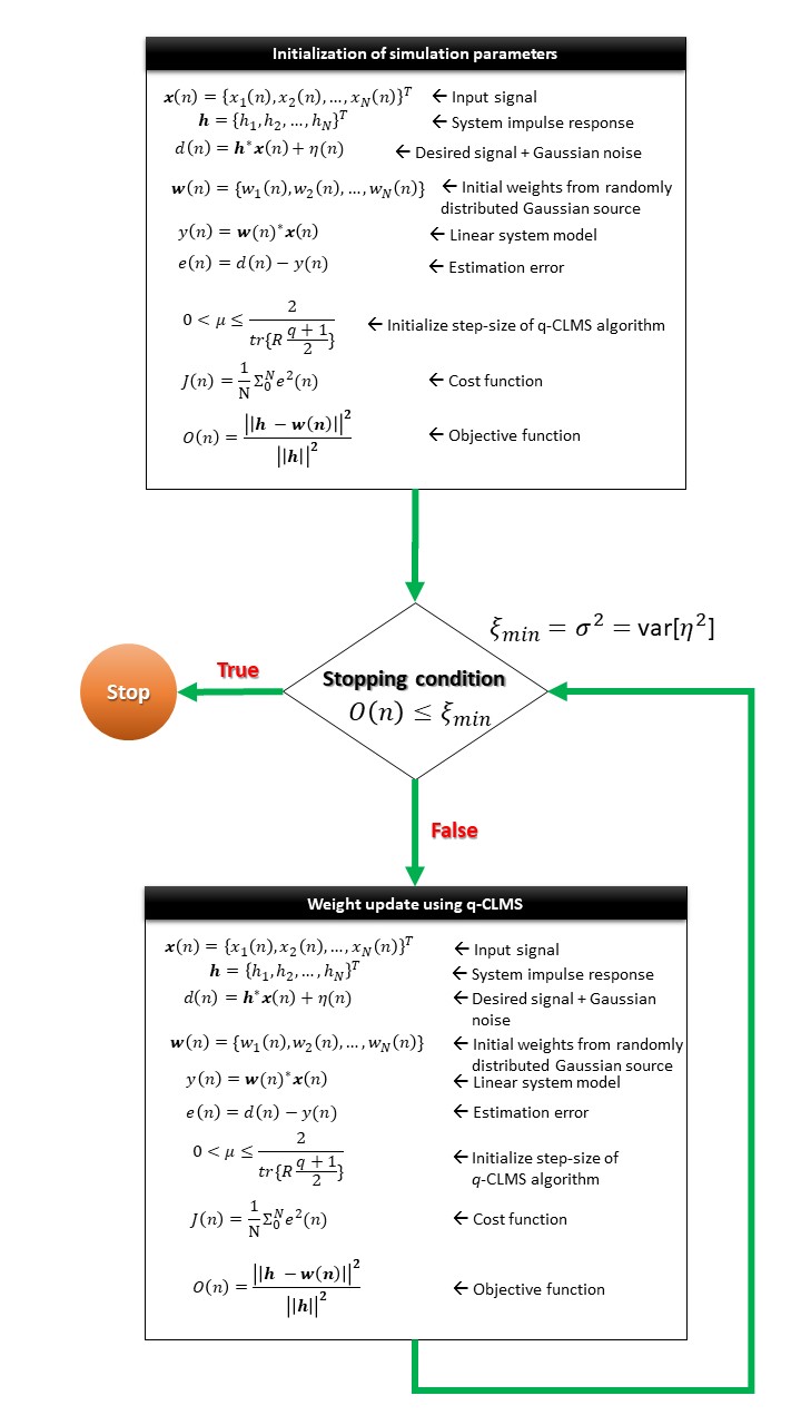
Figure 1: Proposed q-CLMS algorithm-based system identification flowchart

3.1 Optimal Solution of the q-Complex LMS

We explore the optimal solution for $q$-CLMS in this sub-section. As $q$ approaches 1, the $q$-derivative transforms to the standard derivative.
For the optimal solution we replace $\nabla_{q}J(\mathbf{w})(\mathbf{w}^{*}(n))$ in Eq.(33) with zero.

$$-E[(\mathbf{G_{R}}+\mathbf{G_{I}})\mathbf{x}(n)e^{*}(n)]\approx 0$$ (36)

By applying the expectation on Eq.(36) and replacing $e^{*}(n)$ in Eq.(36) we get:

$$(\mathbf{G_{R}}+\mathbf{G_{I}})[\mathbf{P}-\mathbf{R_{x}}\mathbf{w}_{opt}]\approx 0$$ (37)

where $\mathbf{R_{x}}$ is the auto-correlation matrix of the input signal, and $\mathbf{P}$ is defined as the cross-correlation vector of the desired output and input. The optimal weight $\mathbf{w}_{opt}$ is given as:

$$\mathbf{w}_{opt}\approx\mathbf{R_{x}}^{-1}\mathbf{P}$$ (38)

However, the optimal solution is same as the wiener solution.

3.2 Convergence of the Mean

We make the following assumptions for the convenience of analysis:

$1.$

We assume that the real part $\mathbf{x}_{R}(n)$ and the imaginary part $\mathbf{x}_{I}(n)$ are uncorrelated, i.e., $E[\mathbf{x}_{R}(n)\mathbf{x}_{I}(n)]$ = $E[\mathbf{x}_{I}(n)\mathbf{x}_{R}(n)]$ = 0. The input signal auto-correlation matrix is given as: $\mathbf{R_{x}}=E[\mathbf{x}_{R}(n)\mathbf{x}_{R}^{\intercal}(n)]+E[\mathbf{x}_{I}(n)\mathbf{x}_{I}^{\intercal}(n)]$.
For simplicity, we assume that the real and imaginary parts of input signal are identically distributed, therefore, imaginary and real parts of the $\mathbf{G}$ matrix are equal, i.e., $\mathbf{G_{R}}=\mathbf{G_{I}}=\mathbf{G}$

$2.$

The noise sequence $\eta(n)$ is a complex zero-mean process with uncorrelated real and imaginary parts, i.e., $E[\eta(n)]$ = 0, $E[\eta_{R}(n)\eta_{I}(n)]$ = 0.

$3.$

The input vector and noise sequence are also independent $E[\mathbf{x}(n)\eta(n)]=0$ condition

$4.$

The input vector and the weight error vector are independent from each other $E[\mathbf{x}(n)\Delta(n)]$=0

The weight error vector is defined as the difference between the estimated weights and the optimal weights , it is given as:

$$\Delta(n)=\mathbf{w}(n)-\mathbf{w}_{opt}$$ (39)

Under the assumption that the data sequence $\mathbf{x}(n)$ is statistically independent assum1 ; assum4 ; assum5 , the weight and the input vector are statistically independent. The above suppositions are frequently used in the literature ASP . They are used to evaluate the performance analysis of the proposed algorithm.
The quantum calculus based complex form of the LMS algorithm Eq.(35)

$$\mathbf{w}(n+1)=\mathbf{w}(n)+\mu(\mathbf{G_{R}}+\mathbf{G_{I}})\mathbf{x}(n)e^{*}(n)$$ (40)

Now subtracting both sides of Eq.(40) by $\mathbf{w}_{opt}$, the weight-error recursion can be given as $\Delta(n)$

$$\Delta(n+1)=\Delta(n)+\mu(\mathbf{G_{R}}+\mathbf{G_{I}})\mathbf{x}(n)e^{*}(n)$$ (41)

Solving for $\Delta_{R}$, which is the real component of $\Delta(n)$ defined in Eq.(39), substituting the value of $e_{R}(n)$ and $e_{I}(n)$ and applying the expectation results in:

$$\begin{split}&E[\Delta_{R}(n+1)]=\\ &E[\Delta_{R}(n)]-\mu\mathbf{G}_{R}E[\mathbf{x}_{R}(n)\mathbf{x}_{R}^{\intercal}(n)]E[\Delta_{R}(n)]\\ &-\mu\mathbf{G}_{R}E[\mathbf{x}_{I}(n)\mathbf{x}_{I}^{\intercal}(n)]E[\Delta_{R}(n)]\end{split}$$ (42)

$$E[\Delta_{R}(n+1)]=[\mathbf{I}-\mu\mathbf{G}_{R}\mathbf{R_{x}}]E[\Delta_{R}(n)]$$ (43)

and $\mathbf{I}$ is the identity matrix.

$(\mathbf{I}-\mu\mathbf{G}_{R}\mathbf{D})$ is a diagonal matrix

$$\small\mathbf{I}-\mu\mathbf{G}_{R}\mathbf{D}=\begin{bmatrix}1-\mu\frac{(q_{R1}+1)}{2}\lambda_{0}&&\\ &\ddots&\\ &&1-\mu\frac{(q_{RN}+1)}{2}\lambda_{N}\end{bmatrix}$$ (44)

Similarly Eq.(43) can be written as:

$E[\Delta^{{}^{\prime}}_{R}(n+1)]=$

$$\small\begin{bmatrix}(1-\mu\frac{(q_{R1}+1)}{2}\lambda_{0})^{n+1}&&\\ &\ddots&\\ &&(1-\mu\frac{(q_{RN}+1)}{2}\lambda_{N})^{n+1}\end{bmatrix}E[\Delta^{{}^{\prime}}_{R}(0)]$$ (45)

The convergence of the $q$-CLMS algorithm depends on the diagonal elements of Eq.(45) and its absolute value should be less than one.

That is to say

$$\lim_{n\to\infty}|(1-\mu\frac{q_{R}+1}{2}\lambda_{i})^{n+1}|<1,$$

for i=0 …N

$$|(1-\mu\frac{q_{R}+1}{2}\lambda_{Rmax})|<1$$ (46)

where $\lambda_{Rmax}$ is the maximum eigenvalue of the real autocorrelation matrix. The step-size of the $q$-CLMS algorithm must be selected in the range

$$0<\mu<\frac{4}{\lambda_{Rmax}(q_{R}+1)}$$

Similar methodology can be pursued for the imaginary part:

$$E[\Delta_{I}(n+1)]=[\mathbf{I}-\mu\mathbf{G}_{I}\mathbf{R_{x}}]E[\Delta_{I}(n)]$$ (47)

$$0<\mu<\frac{4}{\lambda_{Imax}(q_{I}+1)}$$

Finally, in order for the $q$-CLMS algorithm to converge, it is necessary that both the imaginary parts of its weight error must obey to the condition

$$0<\mu<\frac{4}{max[\lambda_{Rmax}(q_{R}+1),\lambda_{Imax}(q_{I}+1)]}$$ (48)

3.3 Mean Square Analysis

In this section, the mean square analysis of the $q$-CLMS algorithm is carried out. To do so, we take the square of the error and its expectation gives:

$$E[e^{2}(n)]=E[e_{o}(n)-\Delta^{H}(n)\boldsymbol{x}(n)]^{2}$$ (49)

where $H[.]$ is the Hermitian operator and $e_{o}(n)$ is the optimum output error. Upon further simplification, Eq.(49) can be given as

$$E[e^{2}(n)]=e^{2}_{min}+tr[\mathbf{K}^{{}^{\prime}}(n)\mathbf{D}]$$ (50)

where $\mathbf{K}^{{}^{\prime}}(n)$ is the covariance of the weight error vector, $e^{2}_{min}$ is the minimum mean square error and $\mathbf{D}$ is a diagonal matrix.

$$\mathbf{K}^{{}^{\prime}}(n)=\mathbf{T}^{\intercal}cov[\Delta(n)]$$

$$\mathbf{D}=diag\{\lambda_{0},\lambda_{1},\cdots,\lambda_{N}\}$$

where $\mathbf{T}$ is the unitary matrix.
Equation (50) can be expressed as

$$e^{2}(n)=e^{2}_{min}+\sum_{i=1}^{N}\mathbf{K}^{{}^{\prime}}_{ii}(n)\lambda_{i}$$ (51)

where $\lambda_{i}$ represents the eigenvalues of the input signal autocorrelation matrix and $\mathbf{K}^{{}^{\prime}}_{ii}(n)$ shows the diagonal elements of $\mathbf{K}^{{}^{\prime}}(n)$. The $\lambda_{i}$ from the right side of Eq.(51) should be in bound to achieve a minimum error.
For our analysis, the $q$-CLMS algorithm can alternatively be described by:

$$\Delta_{R}(n+1)=\\ \Delta_{R}(n)-\mu\mathbf{G}_{R}\mathbf{x}_{R}(n)\mathbf{x}_{R}^{H}(n)\Delta_{R}(n)+\mu\mathbf{G}_{R}\mathbf{x}_{R}(n)e^{*}_{o}(n)$$ (52)

The covariance of $\Delta_{R}^{{}^{\prime}}(n+1)$ is given as

$$\mathbf{K}_{R}^{{}^{\prime}}(n+1)=E[\Delta_{R}^{{}^{\prime}}(n+1)\Delta_{R}^{{}^{\prime}\intercal}(n+1)]$$ (53)

where $\mathbf{K}_{R}^{{}^{\prime}}(n+1)=cov[\Delta_{R}^{{}^{\prime}}(n+1)]$.
Taking the transpose of Eq.(52)

$$\Delta_{R}^{{}^{\prime}\intercal}(n+1)=\Delta_{R}^{{}^{\prime}\intercal}(n)-\mu\mathbf{G}_{R}\Delta_{R}^{{}^{\prime}\intercal}(n)\mathbf{x}_{R}^{{}^{\prime}*}(n)\mathbf{x}_{R}^{{}^{\prime}\intercal}(n)+\mu\mathbf{G}_{R}e^{H}_{o}(n)\mathbf{x}_{R}^{{}^{\prime}\intercal}(n)$$ (54)

Multiplying Eq.(52) and Eq.(54) to get Eq.(53), we will get 9 terms, and combining all the nine terms results in

$$\mathbf{K}_{R}^{{}^{\prime}}(n+1)=\mathbf{K}_{R}^{{}^{\prime}}(n)-\mu[\mathbf{G}_{R}\mathbf{D}\mathbf{K}_{R}^{{}^{\prime}}(n)\\ +\mathbf{G}_{R}\mathbf{K}_{R}^{{}^{\prime}}(n)\mathbf{D}]+2\mu^{2}\mathbf{G}^{2}_{R}\mathbf{D}\mathbf{K}_{R}^{{}^{\prime}}(n)\boldsymbol{D}\\ +\mu^{2}\mathbf{G}^{2}_{R}\mathbf{D}.tr[\mathbf{D}\mathbf{K}_{R}^{{}^{\prime}}(n)]+\mu^{2}\mathbf{G}^{2}_{R}e^{2}_{min}\mathbf{D}$$ (55)

$\mathbf{D}$ is a diagonal matrix and $e^{2}_{min}$ is the minimum mean square error.

From Eq.(51), it is observable that only the diagonal elements of $\mathbf{K}_{R}^{{}^{\prime}}(n)$ are contributing to the mean square error.

$$\mathbf{K}_{R}^{{}^{\prime}}(n+1)=\mathbf{K}_{R}^{{}^{\prime}}(n)-2\mu\mathbf{G}_{R}\lambda_{i}\mathbf{K}_{R}^{{}^{\prime}}(n)+2\mu^{2}\mathbf{G}^{2}_{R}\lambda_{i}^{2}\mathbf{K}_{R}^{{}^{\prime}}(n)\\ +\mu^{2}\mathbf{G}^{2}_{R}\lambda_{i}\sum\lambda_{i}\mathbf{K}_{R}^{{}^{\prime}}(n)+\mu^{2}\mathbf{G}^{2}_{R}e^{2}_{min}\lambda_{i}$$ (56)

Considering $\lambda$ as a vector having the eigenvalues of $\mathbf{R_{x}}$ and $\mathbf{K}_{R}^{{}^{\prime}}(n+1)$ as a vector having the diagonal elements of $cov[\Delta_{R}(n)]$, the following equation can be formed Eq.(56).

$$\mathbf{K}_{R}^{{}^{\prime}}(n+1)=\Bigg{(}I-2\mu\frac{q_{R}+1}{2}\lambda+2\mu^{2}\Big{(}\frac{q_{R}+1}{2}\Big{)}^{2}\lambda^{2}\\ +\mu^{2}\Big{(}\frac{q_{R}+1}{2}\Big{)}^{2}\lambda\lambda^{\intercal}\Bigg{)}\mathbf{K}_{R}^{{}^{\prime}}(n)+\mu^{2}e^{2}_{min}\Big{(}\frac{q_{R}+1}{2}\Big{)}^{2}\lambda$$ (57)

$$\mathbf{K}_{R}^{{}^{\prime}}(n+1)=\mathbf{B}\mathbf{K}^{{}^{\prime}}_{R}(n)+\mu^{2}e^{2}_{min}\Big{(}\frac{q_{R}+1}{2}\Big{)}^{2}\lambda$$ (58)

here the elements of $\mathbf{B}$ are given by

$$\small b_{ik}=\left\{\begin{array}[]{rcl}\Big{(}1-2\mu\frac{q_{R}+1}{2}\lambda_{i}+2\mu^{2}\big{(}\frac{q_{R}+1}{2}\big{)}^{2}\lambda^{2}_{i}\\ +\mu^{2}\big{(}\frac{q_{R}+1}{2}\big{)}^{2}\lambda^{2}_{i}\Big{)}&for&i=k\\ 2\mu^{2}\big{(}\frac{q_{R}+1}{2}\big{)}^{2}\lambda_{i}\lambda_{k}&for&i\neq k\\ \end{array}\right.$$ (59)

Consequently, a sufficient condition to guarantee convergence is to force the sum of the elements in any row of B to be kept in the range $0<\sum_{k=0}^{N}b_{ik}<1$. Since

$$\sum_{k=0}^{N}b_{ik}=1-2\mu\frac{q_{R}+1}{2}\lambda_{i}+2\mu^{2}\Big{(}\frac{q_{R}+1}{2}\Big{)}^{2}\lambda^{2}_{i}+\mu^{2}\Big{(}\frac{q_{R}+1}{2}\Big{)}^{2}\lambda_{i}\sum_{k=0}^{N}\lambda_{k}$$ (60)

$$0<1-2\mu\frac{q_{R}+1}{2}\lambda_{i}+2\mu^{2}\Big{(}\frac{q_{R}+1}{2}\Big{)}^{2}\lambda^{2}_{i}+\mu^{2}\Big{(}\frac{q_{R}+1}{2}\Big{)}^{2}\lambda_{i}\sum_{k=0}^{N}\lambda_{k}<1$$ (61)

After simplification, the condition of stability is given by:

$$0<\mu<\frac{2}{2\frac{q_{R}+1}{2}\lambda_{i}+\frac{q_{R}+1}{2}\sum_{k=0}^{N}\lambda_{k}}$$

$$0<\mu<\frac{2}{tr[\mathbf{R_{x}}\frac{q_{R}+1}{2}]}$$ (62)

In the same way, the imaginary part can be written as:

$$\mathbf{K}_{I}^{{}^{\prime}}(n+1)=\mathbf{K}_{I}^{{}^{\prime}}(n)-\mu\Big{[}\frac{q_{I}+1}{2}\mathbf{D}\mathbf{K}_{I}^{{}^{\prime}}(n)+\frac{q_{I}+1}{2}\mathbf{K}_{I}^{{}^{\prime}}(n)\mathbf{D}\Big{]}\\ +2\mu^{2}\Big{(}\frac{q_{I}+1}{2}\Big{)}^{2}\mathbf{D}\mathbf{K}_{I}^{{}^{\prime}}(n)\mathbf{D}+\mu^{2}\Big{(}\frac{q_{I}+1}{2}\Big{)}^{2}\boldsymbol{D}.tr[\mathbf{D}\mathbf{K}_{I}^{{}^{\prime}}(n)]\\ +\mu^{2}\Big{(}\frac{q_{I}+1}{2}\Big{)}^{2}e^{2}_{min}\mathbf{D}$$ (63)

$$0<\mu<\frac{2}{tr[\mathbf{R_{x}}\frac{q_{I}+1}{2}]}$$ (64)

where Eq.(62) and (64) are generally used as computation of $tr[\mathbf{R_{x}}]$ is relatively easy to estimate as compared to the estimation of $\lambda_{max}$.

3.4 Excess Mean Square Error (EMSE)

The excess mean square error (EMSE) is the difference between the MSE and minimum MSE. It is considered that the minimal error is reached when the adaptive filter coefficients are frozen at their optimum values. Although the coefficient vector converges to $\mathbf{w}_{opt}$, on average the instantaneous deviation $\Delta(n)=\mathbf{w}(n)-\mathbf{w}_{opt}$, generated by the noisy gradient estimates, causes an excess MSE. From Eq.(49) the square of error is simplified to:

$$\xi(n)=e^{2}_{min}+E[\Delta_{R}^{\intercal}(n)\mathbf{R_{x}}\Delta_{R}(n)]$$ (65)

The excess in MSE is given by

$$\Delta\xi_{exc}(n)\triangleq\xi(n)-e^{2}_{min}=E[\Delta_{R}^{\intercal}(n)\mathbf{R_{x}}\Delta_{R}(n)]$$ (66)

$$=tr\{E[\mathbf{R_{x}}\Delta_{R}(n)\Delta_{R}^{\intercal}(n)]\}$$ (67)

where $tr[\cdot]$ is the trace operator.
Making use of the identity that $\mathbf{TT}^{\intercal}=\mathbf{I}$, the following equation results,

$$\Delta\xi_{exc}(n)=tr\{E[\mathbf{TT}^{\intercal}\mathbf{R_{x}TT}^{\intercal}\Delta_{R}(n)\Delta_{R}^{\intercal}(n)\mathbf{TT}^{\intercal}]\}$$ (68)

$$=tr\{E[\mathbf{TD}\boldsymbol{K}_{R}^{{}^{\prime}}(n)\mathbf{T}^{\intercal}]\}$$ (69)

Therefore,

$$\Delta\xi_{exc}(n)=tr\{E[\mathbf{D}\mathbf{K}_{R}^{{}^{\prime}}(n)]\}$$ (70)

From Eq.(58), it is possible to show that

$$\Delta\xi_{exc}(n)=e^{2}_{min}+\sum_{i=1}^{N}\mathbf{K}^{{}^{\prime}}_{ii}(n)\lambda_{i}$$ (71)

Since,

$$\mathbf{K}_{R,i}^{{}^{\prime}}(n+1)=\\ \Bigg{(}1-2\mu\frac{q_{R}+1}{2}\lambda_{i}+2\mu^{2}\Big{(}\frac{q_{R}+1}{2}\Big{)}^{2}\lambda_{i}^{2}\Bigg{)}\mathbf{K}_{R}^{{}^{\prime}}(n)\\ +\mu^{2}\Big{(}\frac{q_{R}+1}{2}\Big{)}^{2}\lambda_{i}\sum_{k=0}^{N}\lambda_{k}\mathbf{K}_{R,k}^{{}^{\prime}}(n)+\mu^{2}e_{min}^{2}\Big{(}\frac{q_{R}+1}{2}\Big{)}^{2}\lambda_{i}$$ (72)

and $\mathbf{K}_{R,i}^{{}^{\prime}}(n+1)=\mathbf{K}_{R,i}^{{}^{\prime}}(n)$ for large $n$, we can apply a summation operation to Eq.(72) in order to obtain

$$\sum_{k=0}^{N}\lambda_{k}\mathbf{K}_{R,k}^{{}^{\prime}}(n)=\\ \frac{\mu e_{min}^{2}\sum_{i=0}^{N}\frac{q_{R}+1}{2}\lambda_{i}+2\mu\sum_{i=0}^{N}\frac{q_{R}+1}{2}\lambda_{i}^{2}\mathbf{K}_{R,i}^{{}^{\prime}}(n)}{2-\mu\sum_{i=0}^{N}\frac{q_{R}+1}{2}\lambda_{i}}\\ \approx\frac{\mu e_{min}^{2}\sum_{i=0}^{N}\frac{q_{R}+1}{2}\lambda_{i}}{2-\mu\sum_{i=0}^{N}\frac{q_{R}+1}{2}\lambda_{i}}\\ =\frac{\mu e_{min}^{2}tr[\mathbf{R_{x}}\frac{q_{R}+1}{2}]}{2-\mu tr[\mathbf{R_{x}}\frac{q_{R}+1}{2}]}$$ (73)

where the term $2\mu\sum_{i=0}^{N}\frac{q_{R}+1}{2}\lambda_{i}^{2}\mathbf{K}_{R,i}^{{}^{\prime}}(n)$ was considered quite insignificant in comparison to the remaining terms in the numerator. This assumption is difficult to justify, but it holds true for small values of $\mu$. The excess mean-square error can then be expressed as

$$\Delta\xi_{exc}(n)=\lim_{i\to\infty}\frac{\mu\sigma^{2}tr[\mathbf{R_{x}}\frac{q_{R}+1}{2}]}{2-\mu tr[\mathbf{R_{x}}\frac{q_{R}+1}{2}]}$$ (74)

Similarly for imaginary part,

$$\Delta\xi_{exc}(n)=\lim_{i\to\infty}\frac{\mu\sigma^{2}tr[\mathbf{R_{x}}\frac{q_{I}+1}{2}]}{2-\mu tr[\mathbf{R_{x}}\frac{q_{I}+1}{2}]}$$ (75)

In the case where there is a sufficient order of the adaptive filter to model the operation that generated $d(n)$, the minimum MSE attained is equivalent to the variance of the noise added, given by $\sigma^{2}$ .

3.5 Mean Square Deviation (MSD)

The mean square deviation (MSD ) is defined as
$MSD(n)=tr\{E[\mathbf{K}_{R}^{{}^{\prime}}(n+1)]\}$, consequently

$$\small MSD(n+1)=\Bigg{(}I-2\mu\frac{q+1}{2}\lambda+2\mu^{2}\Big{(}\frac{q+1}{2}\Big{)}^{2}\lambda^{2}\\ +\mu^{2}\Big{(}\frac{q+1}{2}\Big{)}^{2}\lambda\lambda^{\intercal}\Bigg{)}MSD(n)+\mu^{2}e^{2}_{min}\Big{(}\frac{q+1}{2}\Big{)}^{2}\lambda$$ (76)

3.6 Misadjustment

The ratio between the excess MSE ($\xi_{exc}$) and the minimum MSE ($\xi_{min}$) is known as the Misadjustment $M$ , the misadjustment is given by

$$M\triangleq\frac{\Delta\xi_{exc}}{e_{min}^{2}}\approx\frac{\mu tr[\mathbf{R_{x}}\frac{q+1}{2}]}{2-\mu tr[\mathbf{R_{x}}\frac{q+1}{2}]}$$ (77)

The analytical results for MSE, EMSE and Misadjustment are summarized in Table.1.

	Analytical Results
	Real	Imaginary
MSE	$0<\mu<\frac{2}{tr[\mathbf{R_{x}}\frac{q_{R}+1}{2}]}$	$0<\mu<\frac{2}{tr[\mathbf{R_{x}}\frac{q_{I}+1}{2}]}$
EMSE	$\frac{\mu\sigma^{2}tr[\mathbf{R_{x}}\frac{q_{R}+1}{2}]}{2-\mu tr[\mathbf{R_{x}}\frac{q_{R}+1}{2}]}$	$\frac{\mu\sigma^{2}tr[\mathbf{R_{x}}\frac{q_{I}+1}{2}]}{2-\mu tr[\mathbf{R_{x}}\frac{q_{I}+1}{2}]}$
Misadjustment	$\frac{\mu tr[\mathbf{R_{x}}\frac{q_{R}+1}{2}]}{2-\mu tr[\mathbf{R_{x}}\frac{q_{R}+1}{2}]}$	$\frac{\mu tr[\mathbf{R_{x}}\frac{q_{I}+1}{2}]}{2-\mu tr[\mathbf{R_{x}}\frac{q_{I}+1}{2}]}$

Table 1: Analytical Results

4 The proposed Enhanced q-CLMS (Eq-CLMS)

The selection of the q-parameter shows greater importance in the performance of $q$-calculus based algorithms. It can be analyzed in sub-section 6.1 of the experimental section. Typically this value is manually chosen. A larger value results in a rapid convergence but yields a larger steady-state error. On the other hand, smaller values of $q$ slow down the convergence while reducing the steady-state error. A trade-off is therefore required by manually choosing a suitable value of the $q$-parameter.

To automate this choice, we modify the proposed $q$-CLMS algorithm by making the $q$-parameter time varying:

$$\mathbf{w}(n+1)=\mathbf{w}(n)+\mu\mathbf{x}(n)e^{*}(n)\odot\mathbf{q}(n)$$ (78)

where $\mathbf{q}(n)$ is the time-varying parameter, which can be calculated by taking the error-correlation energy EqLMS . The proposed algorithm takes large steps for larger error, and decreases the size of the number of steps with a lower error. Highlighting the fact that, the proposed method is absolutely automatic and does not require any other tuning factors as compared to the time-varying $q$-LMS. The proposed update rule for the q-parameter is described below:

• Step1: Initialize by taking any positive random values in vector $\mathbf{q}$ .

• Step2: To update the first entry $q_{1}$ of the vector $\mathbf{q}$, use the instantaneous error related to the weight of the instant input tap, i.e.,

  $$q_{1}(n+1)=\frac{1}{M+1}\{|e(n)|+\sum_{k=1}^{M}\mathbf{q}_{k}(n)\},$$ (79)

  The length of the filter is given by the symbol $M$.

• Step3: In order to maintain fast convergence rate and to avoid divergence, the following conditions will be evaluated:

  $$\mathbf{q}(n+1)=\left\{\begin{array}[]{rcl}\frac{1}{\lambda_{max}}&if&|q_{1}(n+1)|>\frac{1}{\lambda_{max}},\\ q_{1}(n+1)&otherwise,\\ \end{array}\right.$$ (80)

  where $\lambda_{max}$ is the maximum eigenvalue of the input auto-correlation matrix.

• Step4: Except for the first entry, update all entries of the vector $\mathbf{q}$, simply by shifting:

  $$q_{l+1}(n+1)=q_{l}(n),$$ (81)

  where $1<l<M-1$

• Step5: Repeat steps 2 to 5, for next iterations,

Conclusively, the equation for weight-update of the proposed $Eq$-CLMS algorithm can be given as:

$$\mathbf{w}(n+1)=\mathbf{w}(n)+\mu e^{*}(n)\mathbf{x}(n)\odot\mathbf{q}(n),$$ (82)

where $\odot$ indicates the element-wise multiplication.

5 The proposed q-CLMS algorithm as a whitening filter

Due to the spread of eigen values of the input correlation matrix, the convergence speed of LMS algorithm is limited as it shows dependency on eigen values. Explicitly, the time constant $\tau_{a}$ is given as ASP

$$\frac{-1}{ln(1-\mu\lambda_{max})}\leqslant\tau_{a}\leqslant\frac{1}{ln(1-\mu\lambda_{min})}$$ (83)

where $ln$ shows the logarithmic function, and the minimum and maximum eigenvalues of the input correlation matrix are represented by $\lambda_{min}$ and $\lambda_{max}$, respectively.
By taking the above observation into consideration, we established another application of the $q$-gradient. Explicitly, for a faster convergence rate of the LMS algorithm, the $q$ factor can be selected in such a way as to make the LMS filter behaves as a whitening filter (shown in Fig. 10). For evaluation purposes, the transient analyses of the weight error vector of the $q$-CLMS given in Eqs.(43) and (47) is studied. Note that the time constant related with the $m^{th}$ mean weight error tap $\Delta_{R,m}(n)$ is given as

$$\tau_{m}=\frac{-1}{ln(1-\frac{\mu(q_{m}+1)\lambda_{m}}{2})},1\leqslant m\leqslant M$$ (84)

Thus selecting the $q_{m}$ parameter such that

$$\frac{(q_{m}+1)}{2}=\frac{1}{\lambda_{m}}\quad\textrm{or}\quad q_{m}=\frac{2-\lambda_{m}}{\lambda_{m}},1\leqslant m\leqslant M$$ (85)

the time constant $\tau_{m}$ reduces to:

$$\tau_{m}=\frac{-1}{ln(1-\mu)},1\leqslant m\leqslant M$$ (86)

Essentially, by taking the $q$ values as shown in Eq.(85) or by taking $\mathbf{G}$ = $\mathbf{R_{x}}^{-1}$, the $q$-CLMS method vanishes the response of the input correlation matrix. As a result, this will enhance the speed of the proposed method. Eventually, the condition for stability is given by:

$$0<\mu<2\\$$ (87)

5.1 Computational Complexity Analysis

Table 2 shows a comparison of the computational complexity of different variants of CLMS in terms of the number of operations required for the adaptation process.

Method	Operations		Big O
	x	+
CLMS	2M+1	2M	M
NCLMS	3M+2	3M+1	M
CFLMS Shah2017	4M+4	6M	M
FoCLMS Ahmad2021	3M+3	5M	M
q-CLMS	3M+1	2M	M
Eq-CLMS	2M+2	3M+1	M

Table 2: Computational complexities of different algorithms in terms of the number of unknown weights (M)

Let M be the number of unknown filter weights. The CLMS method takes $2M+1$ multiplications and $2M$ additions, while the NCLMS algorithm takes $3M+2$ multiplications and $2M$ additions. Similarly, the CFLMS and FoCLMS, which are fractional variants of LMS, need $4M+4$ and $3M+3$ multiplications and $6M$ and $5M$ additions respectively. Interestingly the proposed quantum calculus based variants of CLMS algorithms, i.e., q-CLMS and Eq-CLMS, require $3M+1$ and $2M+2$ multiplications, and $2M$ and $3M+1$ additions respectively. The proposed Eq-CLMS and q-CLMS require fewer multiplications and additions compared to the NCLMS and fractional variants of the CLMS. In particular, the q-CLMS and Eq-CLMS require $1$ unit and $M$ times fewer multiplications and $M+1$ times fewer additions compared to the NCLMS. Similarly, the q-CLMS and Eq-CLMS require $M+3$ and $2M+2$ fewer multiplications and $4M$ and $3M$ fewer additions compared to the CFLMS. Moreover, FoCLMS requires $2$ units and $M+1$ more multiplications as well as $3M$ and $2M$ times more additions than the proposed q-CLMS and Eq-CLMS algorithm. In an overall sense, the proposed qCLMS and E-qCLMS are shown to be computationally efficient compared to the state-of-the-art relevant approaches.

6 Experimental Setup and Results

The performance of the q-CLMS algorithm is examined in this section for a system identification task. Consider channel estimation shown in Fig. 2.

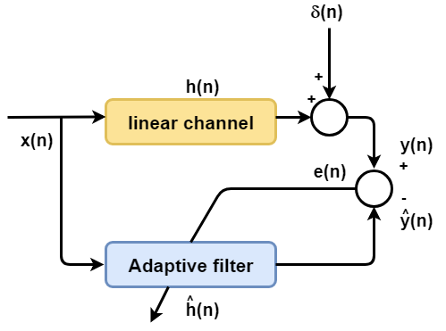
Figure 2: Adaptive learning algorithm based channel estimation.

$$y(n)=h_{1}x(n)+h_{2}x(n-1)+h_{3}x(n-2)+h_{4}x(n-3)+h_{5}x(n-4)$$ (88)

The mathematical model of the system is shown in Eq.(88), it is the FIR filter representation for the adaptive filter block (refer to Fig 2). Where input and output of the system expressed as $\mathbf{x}(n)$ and $y(n)$, respectively. The white Gaussian noise is considered as the disturbance for the system in this case. For experimentation purpose, $\mathbf{x}(n)$ consists of $1\times 10^{3}$ complex randomly generated samples taken from the Gaussian distribution with zero mean and unity variance. The impulse response of the system is given by $\mathbf{h}(n)$ in Eq.(88) while $e(n)$, $\mathbf{\hat{h}}(n)$ and $\hat{y}(n)$ are the estimated error, impulse response and output of the system, respectively. For the performance assessment, the actual and estimated weights are compared by means of the Normalized Weight Deviation (NWD). Explicitly, we define

$$\mbox{NWD}=\frac{\left\|\bf h-\bf w\right\|}{\left\|\bf h\right\|}$$ (89)

where estimated weight-vector is denoted by $\mathbf{w}$ while the actual impulse response of the channel is given by $\mathbf{h}$. For all the simulations, the adaptive filter which is used has the same length as that of the unknown system. The objectives of the simulation are as follows:

$\bullet$

To observe the sensitivity of the proposed method corresponding to the $q$ parameter.

$\bullet$

To validate the derived analytical results for both the steady state and transient analysis.

$\bullet$

To investigate the behavior of the proposed E$q$-CLMS algorithm and compare it with the benchmark algorithms i.e., CLMS, NCLMS and VSS-CLMS.

$\bullet$

To evaluate the performance of the proposed E$q$-CLMS method for correlated imaginary and real components of the system.

$\bullet$

To investigate the behavior of $q$-CLMS as a whitening filter.

$\bullet$

To compare the performance of the proposed Eq-CLMS algorithm with the contemporary approaches i.e., CFLMS and FoCLMS for the channel equalization problem.

6.1 Sensitivity analysis of the q-CLMS algorithm

In this experiment, we observe the sensitivity of the $q$-CLMS algorithm to the $q$ parameter. In particular, we choose a system identification task and study the comparison between the Normalized Weight Difference (NWD) learning curves of the proposed $q$-CLMS algorithm with various $q$ values and compare the results with those obtained via conventional CLMS algorithm (refer to Fig.3). The disturbance which is introduced in the system as a noise is a zero mean i.i.d. sequence with variance 0.01. For convergence the proposed approach took 1000 number of iterations and the mean values are taken for 100 independent runs. We evaluated five different values of $q$ which are $0.5$ , $1$, $2$, $4$, and $8$ for the $q$-CLMS algorithm . Figure 3 clearly shows that for $q=1$ the learning curve exactly matches with the conventional CLMS method showing that for $q=1$ the algorithm shows the conventional CLMS case. It is observable that for greater values of $q$, the proposed $q$-CLMS algorithm exhibits a faster convergence accompanied with a larger steady-state error. Whereas for smaller values of $q$, a comparatively smaller steady-state error is reported but with a slower convergence.

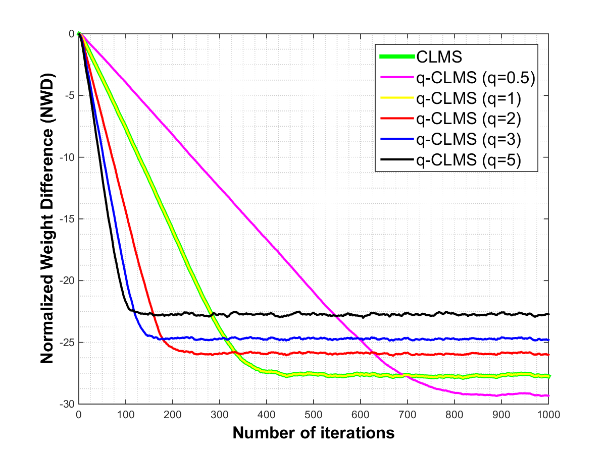
Figure 3: NWD behaviour for the proposed $q$-CLMS and the conventional CLMS algorithm.

6.2 Validation of analytical results of the proposed q-CLMS algorithm

To validate our theoretical findings, we compare the the derived analytical results with the simulation results. The $q$-CLMS algorithm’s transient and steady-state performances are essentially examined. For two choices of the step-size i.e., 0.01 and 0.001, experimental MSE learning curves are compared to those generated using the derived expression in Eq.(57). The algorithm took 10000 iterations to reach convergence, and the mean value was obtained from 1000 independent runs. For both large and small step-size values, Fig.4 indicates an outstanding match between theory and simulation. The step-size values are compared to the simulation findings in the second experiment shown in Fig.5, which are plotted against the analytical values of the steady-state EMSE determined in Eq.(74). The relationship between the theoretical and simulation results is also shown in Fig. 5.

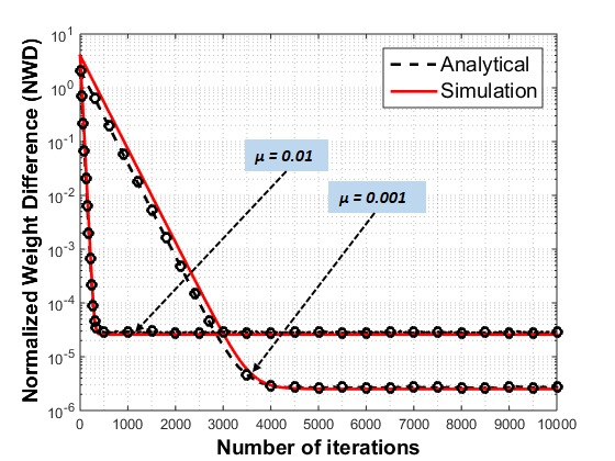
Figure 4: Simulation and analytical MSE behavior of the $q$-CLMS algorithm: For $\mu=0.01$ and $\mu=0.001$.

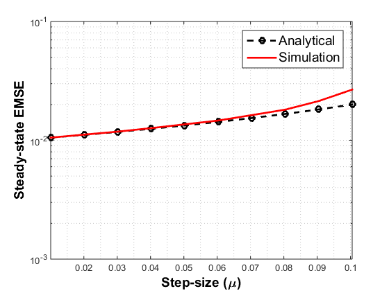
Figure 5: Simulation and analytical EMSE behavior of the $q$-CLMS algorithm: Excess MSE gradually increase with increase in step-size.

6.3 Performance of the proposed Eq-CLMS algorithm

In this set of experiments, we evaluate the performance of the E$q$-CLMS algorithm as derived in Section 4. Essentially the self-regulating technique, proposed in Eqs.(80) and (81), provides an automatic adjustment. The experiment is implemented with five different SNR levels of $2$ dB, $5$ dB, $10$ dB. $20$ dB and $30$ dB. Note that the proposed E$q$-CLMS algorithm is completely automatic and does not require a hard-coded value of the $q$ parameters. By virtue of the recursions proposed in Eqs.(80) and (81), the entries of $\mathbf{q}$ are automatically regularized to attain the best performance. For our experiments, an initialization of $\mathbf{q}=[1\ 1\ 1\ 1\ 1]$ is adopted.
Figure 7 shows the performance of the proposed Eq-CLMS algorithm when operating on five different noise levels. The proposed Eq-CLMS algorithm obtained the lowest steady-state error of $-25.13$ dB when operating on the highest value of SNR i.e., $30$ dB, while the contemporary approaches CLMS, NCLMS and VSS-CLMS achieved higher steady-state values of $-20.82$ dB, $-18.5$ dB and $-20.03$ dB, respectively. For the lowest SNR which is $2$ dB, the proposed Eq-CLMS algorithm outperformed the conventional CLMS and VSS-CLMS algorithm by a margin of $2$ dB and NCLMS by a margin of $3.938$ dB. Similarly for $5$, $10$ and $20$ dB the lowest steady-state error is achieved by the proposed Eq-CLMS algorithm i.e, $-9.912$ dB, $-12.37$ dB and $-17.39$ dB respectively. Steady-state error attained for five different noise levels for CLMS, NCLMS, VSS-CLMS and Eq-CLMS algorithms are summarized in table 3. To show the adaptivity of q parameter, in Figure 6 for 30 dB noise level we showed the values of q for each update iteration.

Table 3: Comparison of steady-state performance

Algorithms	SNR Values (dB)
	2	5	10	20	30
CLMS	-6.87	-8.32	-10.75	-15.79	-20.82
NCLMS	-4.521	-5.929	-8.39	-13.92	-18.5
VSS-CLMS	-6.07	-7.48	-9.949	-15.01	-20.03
Eq-CLMS	-8.459	-9.912	-12.37	-17.39	-25.13

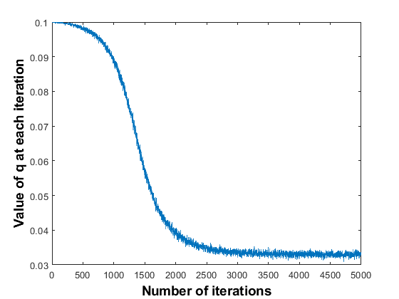
Figure 6: The value of q after each iteration when operating on the SNR value of 30 dB.

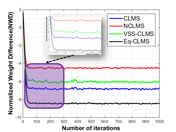
(a)

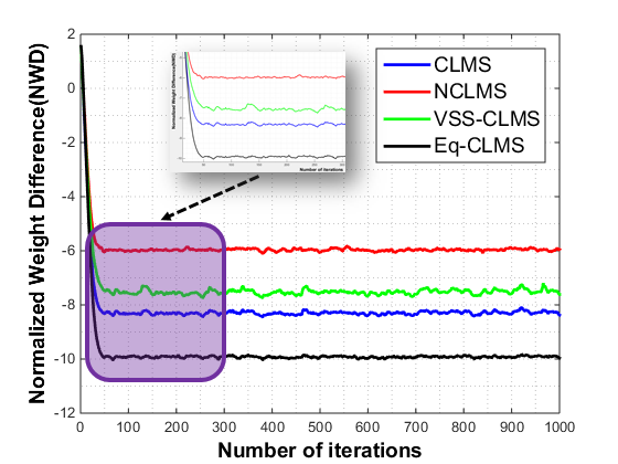
(b)

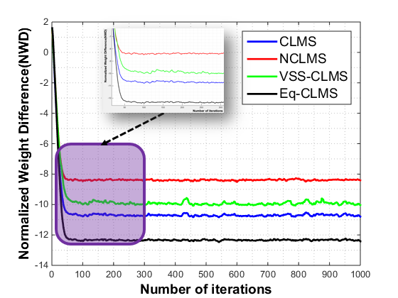
(c)

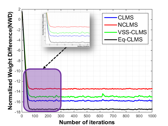
(d)

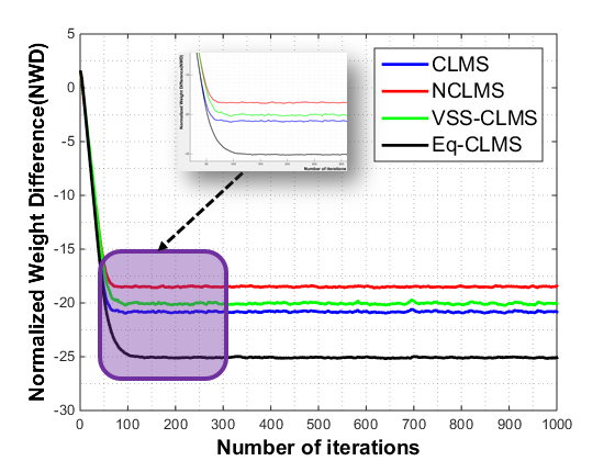
(e)

Figure 7: NWD curves for the CLMS, NCLMS, VSS-CLMS, and the proposed $Eq$-CLMS algorithm with the SNR of (a) $2$ dB, (b) $5$ dB,(c) $10$ dB, (d) $20$ dB, and (e) $30$ dB.

6.4 Complex signal with correlated real and imaginary data

In this experiment, we evaluate the performance of the proposed algorithm for complex data with correlated imaginary and real parts. The complex input signal $\mathbf{x}(n)$ of size $1\times 5000$ was taken from the non-Gaussian distribution with correlated imaginary and real parts and impulse response of the system $\mathbf{h}(n)$ was taken to be complex randomly generated samples of size $1\times 5$. Experiments were performed for both q-CLMS and Eq-CLMS algorithms, simulations were run for $5000$ iterations and the mean results were computed for 1000 independent runs.

To evaluate the proposed q-CLMS algorithm, a fixed value for the G matrix i.e, $\mathbf{q}=[3\ 3\ 3\ 3\ 3]$ is taken. The proposed q-CLMS algorithm attained the lowest steady-state error of $-23.28$ dB whereas the conventional CLMS algorithm attained a larger value of $-21.44$ dB.

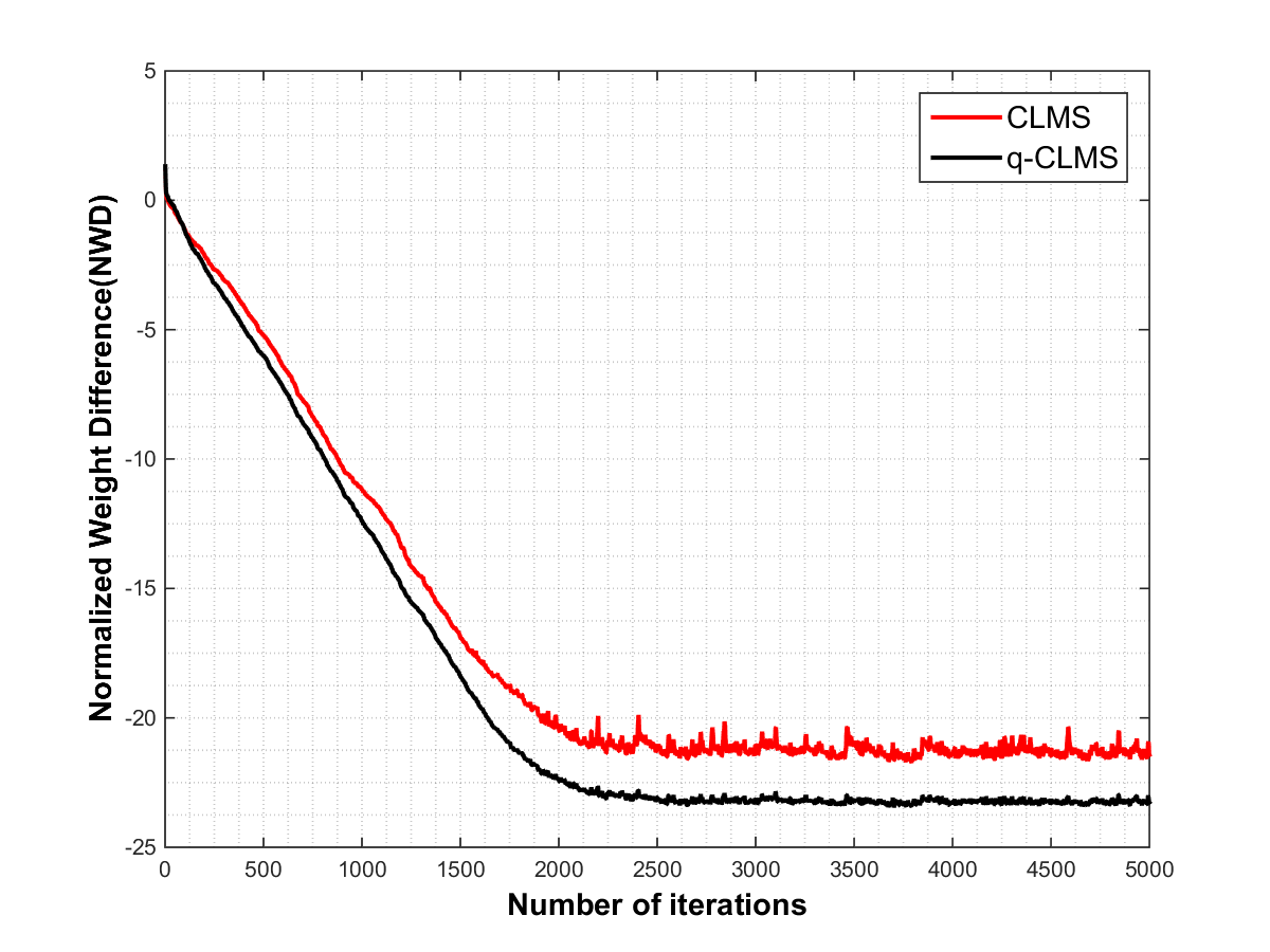
Figure 8: Performance curve for data having correlated real and imaginary parts with a fixed $\mathbf{G}$ matrix.

The second set of experiments was conducted using an adaptive ’q’ parameter, an initial value of $\mathbf{q}=[0.02\ 0.02\ 0.02\ 0.02\ 0.02]$ was adopted. The proposed Eq-CLMS method attained the least steady-state error of $-25$ dB whereas the conventional CLMS algorithm attained a larger value of $-20.8$ dB.

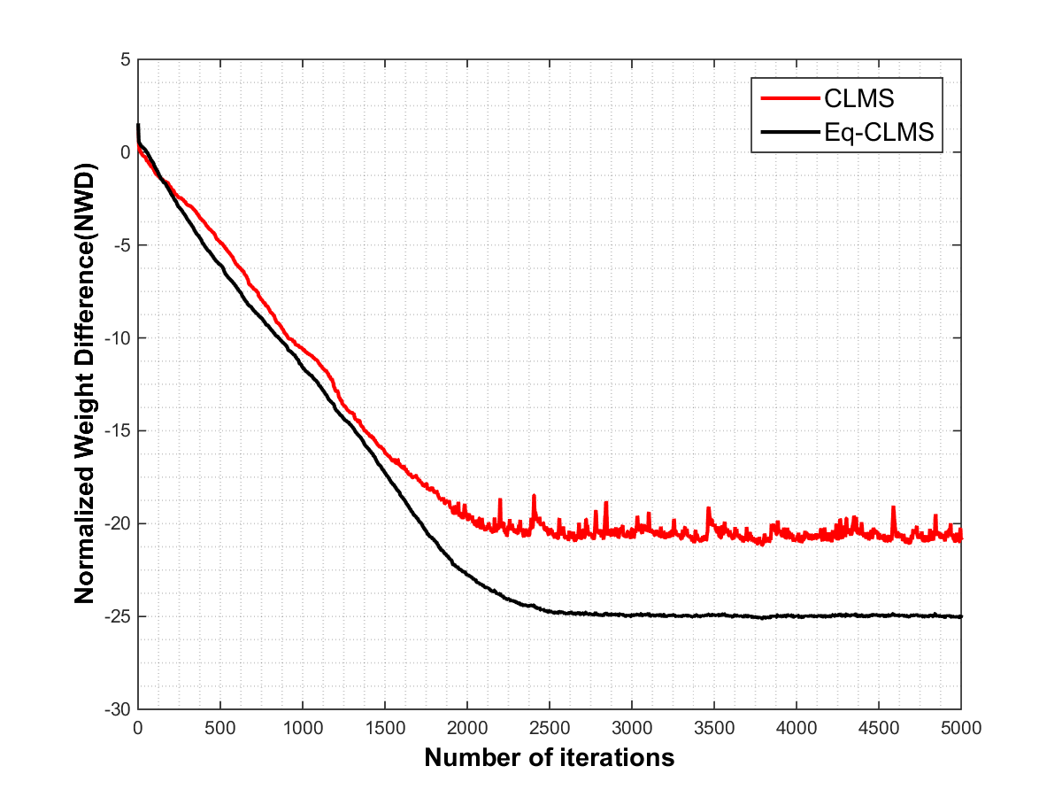
Figure 9: Performance curve for correlated complex signal with varying q-parameter.

6.5 Whitening behavior of the proposed q-CLMS algorithm

Figure 10: System identification and whitening filter.

This section examines the whitening behavior of the $q$-CLMS algorithm. A graphical model of the system identification with adaptive whitening filter is shown in Figure 10. As mentioned in section 5, the q-CLMS algorithm vanished the effect of the input correlation. A non-Gaussian input signal is considered to evaluate the whitening behavior of the proposed $q$-CLMS algorithm. For convergence the algorithm took 10000 iterations and the mean value is taken for 100 independent runs. The NWD learning curve of the q-CLMS method ($\mathbf{G}$ = $\mathbf{R_{x}}^{-1}$) is compared to those of the conventional CLMS and NCLMS methods in Fig.11. From the results, it can be seen that the CLMS and the NCLMS algorithms achieve equal steady-state error of $-29.26$ dB in $2600$ iterations, approximately. The proposed q-CLMS (as a whitening filter) comprehensively outperforms the two competitors, achieving the same steady state error of $-29.26$ dB in $500$ iterations only which is $5.2\times$ faster than the two competitors. The use of Eq.(85) to select the $q$ parameter allows the $q$-CLMS method to converge regardless of the input correlation, as explained in Section 5. Furthermore, the results in Figure 11 supported the claim for two extreme values of the correlation factor, $\sigma xx$ = $0.99$ and $\sigma xx$ = $0.1$, the $q$-CLMS method with whitening $q$ selection is simulated. The whitening $q$ selection ensures that the $q$-CLMS algorithm’s convergence is independent of the input correlation, as shown in Figure 11.

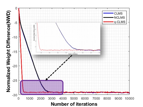
Figure 11: Comparison of the NWD behaviour of the whitening $q$-CLMS and the conventional CLMS algorithm: The proposed approach took $1750$ less number of iterations compared to CLMS and NCLMS.

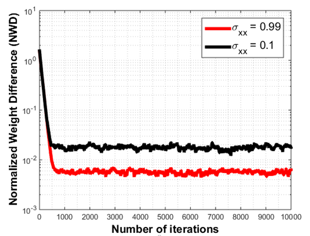
Figure 12: NWD behaviour of the whitening $q$-CLMS for two extreme values of input variances i.e., $\sigma_{xx}=0.99$ and $\sigma_{xx}=0.1$. Note that the rate of convergence of the q-CLMS is same for both input distributions.

6.6 Comparative analysis of the proposed Eq-CLMS algorithm for the problem of channel equalization

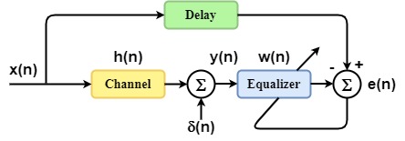
Figure 13: Adaptive channel equalization.

Algorithm	Convergence point (number of iterations x 5000)
	30 dB SNR	40 dB SNR
CLMS	103	110
CFLMS (0.9)	110	111
CFLMS (0.75)	121	127
FoCLMS (0.9)	100	100
FoCLMS (0.75)	149	150
Eq-CLMS	51	52

Table 4: The Convergence point of various approaches including CLMS, CFLMS, FoCLMS (for two distinct values of fractional power i.e., 0.75 and 0.9) and the proposed Eq-CLMS algorithm.

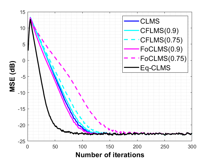
(a)

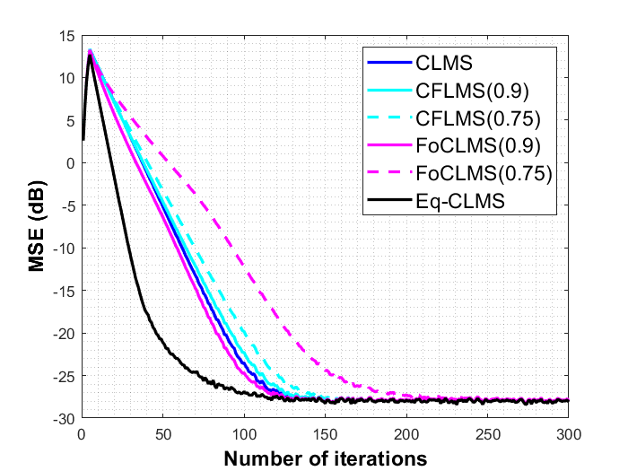
(b)

Figure 14: MSE curves for the CLMS, CFLMS (f = 0.75 and 0.9), FoCLMS (f = 0.75 and 0.9), and the proposed $Eq$-CLMS algorithm with the SNR of (a) $10$ dB and (b) $20$ dB.

The performance of the proposed Eq-CLMS algorithm is evaluated for the problem of channel equalization (refer to Figure 13). The transmitted data $\mathbf{x}(n)$ consisting of $3\times 10^{2}$ complex randomly generated samples drawn from the standard Gaussian distribution, is passed through the channel modeled as a finite impulse response (FIR) filter. The size of the channel is taken to be $1\times 5$ initialized by taking all ones and the weights initialized randomly. Zero-mean additive white Gaussian noise (AWGN) is added to the channel output. To cancel the effects of the channel, the noisy signal is sent to the equalizer and the weights of the equalizer are updated through an adaptive algorithm. For the modulation of input signal binary phase-shift keying (BPSK) is used and the error is calculated by taking the difference between the true output (equalized signal) and the desired response (original input signal). For the performance assessment, mean squared error (MSE) is used given as

$$\text{MSE}=\frac{1}{n}\sum_{i=1}^{n}(e(n))^{2}$$ (90)

where $n$ represents the number of data points and $e$ is the error generated between the true and desired signal.

Performance of the proposed Eq-CLMS approach is compared with three contemporary methods namely: (1) complex LMS (CLMS), (2) fractional CLMS, and (3) fractional order complex LMS (FoCLMS). The experiments are conducted on two different SNR levels of $10$ dB and $20$ dB with step-sizes of $2e^{-3}$, $1e^{-3}$, $2.5e^{-3}$, and $1.5e^{-2}$ for CLMS, CFLMS, FoCLMS, and Eq-CLMS, respectively. The hyper-parameters of all methods are set to achieve similar steady-state-error. For fractional variants, two fractional powers are chosen i.e., $0.9$ and $0.75$ and the simulations are run for $300$ iterations, mean results are reported for $1000$ independent runs. Comprehensive results are tabulated in Table 4. The MSE curves for CLMS, CFLMS, FoCLMS, and the proposed Eq-CLMS algorithms are shown in Figure 14. The proposed Eq-CLMS algorithm is shown to have the fastest convergence rate for both values of SNR. For fractional power of $0.75$ and $0.9$, the CFLMS has the slowest convergence rate at both SNR levels. Furthermore, CLMS and FoCLMS show faster convergence when compared to CFLMS, but slower when compared to the proposed technique. In particular, the proposed Eq-CLMS algorithm achieved the fastest convergence at $51^{th}$ and $52^{th}$ iterations for $10$ dB and $20$ dB SNR respectively. This performance is $2.01$ and $2.11$ times faster compared to the CLMS algorithm for the two SNR levels respectively. In comparison to the fractional variants of CLMS for two different values of fractional power i.e., $0.9$ and $0.75$, the CFLMS requires $59$ and $70$ more iterations for $10$ dB SNR level. For $20$ dB SNR it requires $59$ and $75$ more iteration compared to the proposed Eq-CLMS algorithm. The FoCLMS algorithm requires $49$ and $98$ more iterations (corresponding to fractional powers of 0.9 and 0.75 respectively) for $10$ dB SNR and $48$ and $98$ more iterations (corresponding to fractional powers of 0.9 and 0.75 respectively) for $20$ dB SNR compared to the proposed approach. Results are summarized in Table 4. These results comprehensively demonstrate the superiority of the proposed algorithm in terms of convergence rate.

7 Conclusion

In this work, a novel adaptive algorithm for complex domain has been presented. The proposed algorithm, called the q-CLMS algorithm, is based on q-calculus and makes use of the Wirtinger method. Through the $q$ parameter, the proposed method offers more control over the steady-state and convergence performances compared to the contemporary approaches. The transient and steady-state analyses of the proposed algorithm were carried out and theoretical findings are found to be in agreement with the simulation results. The proposed concept is further automated through an adaptive approach called as enhanced q-CLMS (Eq-CLMS). The enhanced approach automatically selects the best value of the ’q’ parameter without requiring the hit and trial approach. Extensive experiments have been conducted on three significant problems namely: (1) System identification, (2) whitening filter, and (3) channel equalization. The proposed algorithm has shown superior performance compared to the contemporary approaches.

Compliance with ethical standards

Conflict of interest The authors declared that they have no conflict of interest to this work.

References

- [1] Juan Manuel Górriz, Javier Ramírez, S Cruces-Alvarez, Carlos G Puntonet, Elmar W Lang, and Deniz Erdogmus. A novel LMS algorithm applied to adaptive noise cancellation. IEEE Signal Processing Letters, 16(1):34–37, 2009.
- [2] Sandeep Singh, Alaknanda Ashok, Manjeet Kumar, and Tarun Kumar Rawat. Adaptive infinite impulse response system identification using teacher learner based optimization algorithm. Applied Intelligence, 49(5):1785–1802, May 2019.
- [3] Cao Van Kien, Ho Pham Huy Anh, and Nguyen Ngoc Son. Adaptive inverse multilayer fuzzy control for uncertain nonlinear system optimizing with differential evolution algorithm. Applied Intelligence, 51(1):527–548, Jan 2021.
- [4] Bunyodbek Ibrokhimov, Cheonghwan Hur, Hyunseok Kim, and Sanggil Kang. A-dbnf: adaptive deep belief network framework for regression and classification tasks. Applied Intelligence, Jan 2021.
- [5] Xinping Wu, Hongmei Chen, Tianrui Li, and Jihong Wan. Semi-supervised feature selection with minimal redundancy based on local adaptive. Applied Intelligence, Apr 2021.
- [6] Baihua Chen, Yunlong Gao, Shunxiang Wu, Jinyan Pan, Jinghua Liu, and Yuling Fan. Soft adaptive loss based laplacian eigenmaps. Applied Intelligence, Apr 2021.
- [7] Zongyuan Ding, Tao Wang, Quansen Sun, and Hongyuan Wang. Adaptive fusion with multi-scale features for interactive image segmentation. Applied Intelligence, Jan 2021.
- [8] Canlin Li, Jinhua Liu, Qinge Wu, and Lihua Bi. An adaptive enhancement method for low illumination color images. Applied Intelligence, 51(1):202–222, Jan 2021.
- [9] Scott C Douglas. A family of normalized LMS algorithms. IEEE Signal Processing Letters, 1(3):49–51, 1994.
- [10] Rahul Yedida, Snehanshu Saha, and Tejas Prashanth. Lipschitzlr: Using theoretically computed adaptive learning rates for fast convergence. Applied Intelligence, Sep 2020.
- [11] Shujaat Khan, Muhammad Usman, Imran Naseem, Roberto Togneri, and Mohammed Bennamoun. VP-FLMS: a Novel Variable Power Fractional LMS Algorithm. In 2017 Ninth International Conference on Ubiquitous and Future Networks (ICUFN) (ICUFN 2017), Milan, Italy, July 2017.
- [12] Jawwad Ahmad, Muhammad Usman, Shujaat Khan, Imran Naseem, and Hassan Jamil Syed. RVP-FLMS : A Robust Variable Power Fractional LMS Algorithm. In 2016 IEEE International Conference on Control System, Computing and Engineering (ICCSCE). IEEE, 2016.
- [13] Shujaat Khan, Muhammad Usman, Imran Naseem, Roberto Togneri, and Mohammad Bennamoun. A Robust Variable Step Size Fractional Least Mean Square (RVSS-FLMS) Algorithm. In 13th IEEE Colloquium on Signal Processing and its Applications (CSPA 2017). IEEE, 2017.
- [14] R. H. Kwong and E. W. Johnston. A variable step size LMS algorithm. IEEE Transactions on Signal Processing, 40(7):1633–1642, Jul 1992.
- [15] Ubaid M. Al-Saggaf, Muhammad Moinuddin, Muhammad Arif, and Azzedine Zerguine. The q-Least Mean Squares algorithm. Signal Processing, 111(Supplement C):50 – 60, 2015.
- [16] Muhammad Usman, Muhammad Sohail Ibrahim, Jawwad Ahmed, Syed Saiq Hussain, and Muhammad Moinuddin. Quantum calculus-based volterra lms for nonlinear channel estimation. In 2019 Second International Conference on Latest trends in Electrical Engineering and Computing Technologies (INTELLECT), pages 1–4, 2019.
- [17] A. U. Al-Saggaf, M. Arif, U. M. Al-Saggaf, and M. Moinuddin. The q-normalized least mean square algorithm. In 2016 6th International Conference on Intelligent and Advanced Systems (ICIAS), pages 1–6, Aug 2016.
- [18] Shashi Kant Mishra, Suvra Kanti Chakraborty, Mohammad Esmael Samei, and Bhagwat Ram. A q-polak–ribière–polyak conjugate gradient algorithm for unconstrained optimization problems. Journal of Inequalities and Applications, 2021(1):1–29, 2021.
- [19] Syed Saiq Hussain, Muhammad Usman, Taha Hasan Masood Siddique, Imran Naseem, Roberto Togneri, and Mohammed Bennamoun. q-rbfnn: A quantum calculus-based rbf neural network. arXiv preprint arXiv:2106.01370, 2021.
- [20] Alishba Sadiq, Shujaat Khan, Imran Naseem, Roberto Togneri, and Mohammed Bennamoun. Enhanced q-least mean square. Circuits, Systems, and Signal Processing, 38(10):4817–4839, Oct 2019.
- [21] Alishba Sadiq, Muhammad Usman, Shujaat Khan, Imran Naseem, Muhammad Moinuddin, and Ubaid M Al-Saggaf. q-lmf: Quantum calculus-based least mean fourth algorithm. In Fourth International Congress on Information and Communication Technology, pages 303–311. Springer, 2020.
- [22] D. P. Mandic, S. Javidi, G. Souretis, and V. S. L. Goh. Why a complex valued solution for a real domain problem. In 2007 IEEE Workshop on Machine Learning for Signal Processing, pages 384–389, Aug 2007.
- [23] Shujaat Khan, Jaeyoung Huh, and Jong Chul Ye. Adaptive and compressive beamforming using deep learning for medical ultrasound. IEEE Transactions on Ultrasonics, Ferroelectrics, and Frequency Control, pages 1–1, 2020.
- [24] I. Scott. Development of a complete radar system model. In Proceedings of the 2001 IEEE Radar Conference (Cat. No.01CH37200), pages 35–40, 2001.
- [25] R. Falahian, M. M. Dastjerdi, and S. Gharibzadeh. Authentic modeling of complex dynamics of biological systems by the manipulation of artificial intelligence. In 2015 The International Symposium on Artificial Intelligence and Signal Processing (AISP), pages 47–52, March 2015.
- [26] I. Džafić, R. A. Jabr, and T. Hrnjić. High performance distribution network power flow using wirtinger calculus. IEEE Transactions on Smart Grid, pages 1–1, 2018.
- [27] Md. Faijul Amin, Muhammad Ilias Amin, A. Y. H. Al-Nuaimi, and Kazuyuki Murase. Wirtinger calculus based gradient descent and levenberg-marquardt learning algorithms in complex-valued neural networks. In Bao-Liang Lu, Liqing Zhang, and James Kwok, editors, Neural Information Processing, pages 550–559, Berlin, Heidelberg, 2011. Springer Berlin Heidelberg.
- [28] P. Bouboulis and S. Theodoridis. Extension of wirtinger’s calculus to reproducing kernel hilbert spaces and the complex kernel lms. IEEE Transactions on Signal Processing, 59(3):964–978, March 2011.
- [29] Bernard Widrow, John McCool, and Michael Ball. The complex LMS algorithm. Proceedings of the IEEE, 63(4):719–720, April 1975.
- [30] Azam Khalili, Amir Rastegarnia, Wael M Bazzi, and Zhi Yang. Derivation and analysis of incremental augmented complex least mean square algorithm. IET Signal Processing, 9(4):312–319, 2015.
- [31] Azam Khalili, Amir Rastegarnia, and Saeid Sanei. Quantized augmented complex least-mean square algorithm: Derivation and performance analysis. Signal Processing, 121:54–59, 2016.
- [32] J. Ahmad, S. Khan, M. Usman, I. Naseem, M. Moinuddin, and H. J. Syed. Fclms: Fractional complex lms algorithm for complex system identification. In 2017 IEEE 13th International Colloquium on Signal Processing its Applications (CSPA), pages 39–43, March 2017.
- [33] Y. Xia, S. Javidi, and D. P. Mandic. A regularised normalised augmented complex least mean square algorithm. In 2010 7th International Symposium on Wireless Communication Systems, pages 355–359, Sept 2010.
- [34] Syed Muslim Shah, Raza Samar, Noor M. Khan, and Muhammad Asif Zahoor Raja. Design of fractional-order variants of complex lms and nlms algorithms for adaptive channel equalization. Nonlinear Dynamics, 88(2):839–858, Apr 2017.
- [35] Jawwad Ahmad, Muhammad Zubair, Syed Sajjad Hussain Rizvi, and Muhammad Shafique Shaikh. Design and analysis of the fractional-order complex least mean square (foclms) algorithm. Circuits, Systems, and Signal Processing, Apr 2021.
- [36] Tulay Adali Simon S.Haykin. Adaptive Signal Processing: Next Generation Solutions. Wiley, 2010.
- [37] Thomas Ernst. A Comprehensive Treatment of q-Calculus. Springer Science & Business Media, Basel, 1 edition, 2012.
- [38] Gaspard Bangerezako. Variational q-calculus. Journal of Mathematical Analysis and Applications, 289(2):650 – 665, 2004.
- [39] Jessada Tariboon, Sotiris K. Ntouyas, and Praveen Agarwal. New concepts of fractional quantum calculus and applications to impulsive fractional q-difference equations. Advances in Difference Equations, 2015(1):18, Jan 2015.
- [40] Jessada Tariboon and Sotiris K. Ntouyas. Quantum calculus on finite intervals and applications to impulsive difference equations. Advances in Difference Equations, 2013(1):282, Nov 2013.
- [41] Victor Kac and Pokman Cheung. Quantum Calculus. Springer New York, 2012.
- [42] J. Koekoek and R. Koekoek. A note on the q-derivative operator. ArXiv Mathematics e-prints, August 1999.
- [43] Raphael Hunger. An introduction to complex differentials and complex differentiability. Technical report, Technische Universitat¨ Munchen, 2007.
- [44] G. Su, J. Jin, Y. Gu, and J. Wang. Performance analysis of norm constraint least mean square algorithm. IEEE Transactions on Signal Processing, 60(5):2223–2235, May 2012.
- [45] J. Treichler. Transient and convergent behavior of the adaptive line enhancer. IEEE Transactions on Acoustics, Speech, and Signal Processing, 27(1):53–62, February 1979.
- [46] J. Rickard and J. Zeidler. Second-order output statistics of the adaptive line enhancer. IEEE Transactions on Acoustics, Speech, and Signal Processing, 27(1):31–39, February 1979.
- [47] B. Fisher and N. Bershad. The complex lms adaptive algorithm–transient weight mean and covariance with applications to the ale. IEEE Transactions on Acoustics, Speech, and Signal Processing, 31(1):34–44, 1983.