Steady state of overdamped particles in the non-conservative force field of a simple non-linear model of optical trap

Abstract

Optically trapped particles are often subject to a non-conservative scattering force arising from radiation pressure. In this paper we present an exact solution for the steady state statistics of an overdamped Brownian particle subjected to a commonly used force field model for an optical trap. The model is the simplest of its kind that takes into account non-conservative forces. In particular, we present exact results for certain marginals of the full three dimensional steady state probability distribution as well as results for the toroidal probability currents which are present in the steady state, as well as for the circulation of theses currents. Our analytical results are confirmed by numerical solution of the steady state Fokker-Planck equation.

Optical traps and tweezers developed by Ashkin in the 1970s and 1980s ashkin1970 ; ashkin2006 enable the trapping and the manipulation of nano-size particles. These optical set-ups have been used to measure very small forces in a wide range of systems, including living cells ashkin1987 (e.g. virus, bacteria, proteins, and biopolymers), colloids grier1997 ; lukic2007 ; jop2009 , dielectric and metallic nanoparticles dienerowitz2008 ; gieseler2012 ; li2013 ; bateman2014 ; lehmuskero2015 and ultra-cold atoms wildermuth2004 . Optical traps also have many applications, ranging from physics to biology. For instance, they have allowed the characterization of the elasticity of DNA strands chu1991 ; wang1997 ; bustamante2000 ; huguet2010 ; wen2007 ; ritort2006 , the measurement of ultraweak force intensity moore2014 ; ranjit2016 ; liu2017 and have lead to propositions for the detection of gravitational waves arvanitaki2013 and dark energy rider2016 . They have also been useful to experimentally verify some theoretical results in out-of-equilibrium statistical mechanics, such as the fluctuation-dissipation theorem collin2005 ; carberry2004 ; carberry2007 ; berut2016 , as well as in quantum mechanics bassi2013 . In many of these cases, the system is forced out-of equilibrium by moving the trap center.

In the majority of the studies mentioned above, the optical trap is considered to be harmonic. However the trap range is obviously finite and the potential decreases far from the center of the laser beam and is thus generally anharmonic. Another reason for anharmonicity comes from the radiation pressure of the laser which generates a non-conservative component to the force. The importance of this non-conservative component has recently been demonstrated wu2009 . The presence of scattering forces means that even static optical traps acting on Brownian particles lead to an out-of-equilibrium system which is not described by a Gibbs-Boltzmann probability distribution, and notably has non-zero steady state currents. When the particle motion is overdamped, both experimental and theoretical studies roichmann2008 ; sun2009 ; sun2010 ; simpson2010 ; moyses2015 ; demessieres2011 have shown that the current lines take the form of a torus, whose axis is the center of the laser beam. Similar toroidal currents have been uncovered in the underdamped regime via experimental and theoretical analysis amarouchene2019 ; mangeat2019 . In all these cases, analytical expressions for the stationary density and current have, to date, only been derived in a perturbative approach assuming small non-conservative forces moyses2015 ; mangeat2019 . In fact, even in the simplest non-trivial model including scattering forces, the motion in the longitudinal direction is driven by a colored and non-Gaussian noise. This aspect is a major obstacle towards analytical non-perturbative theories which we wish to address in this paper. More generally, our study is an example of a characterization of currents in non-equilibrium steady states, an open problem of non-equilibrium statistical mechanics liver2020 .

In this article, we study the stationary state of overdamped Brownian particles in optical traps, in presence of a non-conservative force component created by the radiation pressure of the laser. In Section I, we first present the basic model for the optical trapping forces and then present the Langevin dynamics for the trapped particle in the overdamped limit. We consider the trapping potential to be composed of a harmonic, conservative, component along with the leading order non-conservative force derived with the paraxial approximation. As well as being of direct relevance to the important field of optical trapping, the model studied constitutes a minimal model of a system which is non-equilibrium due to the presence of non-conservative forces. In particular the non-conservative force is non-Gaussian and this renders the analysis of the steady state more difficult as it cannot be simply characterized in terms of the first two moments. We show how the components of the trapped particle motion can be decomposed into motions subject to conservative forces and motions subject to non-conservative forces. In particular we define an effective two dimensional non-equilibrium process, the steady statistics of which can be used to determine the steady state statistics of the full model. In Section II, we show how the equilibrium distribution of the effective two dimensional process can be extracted from its Fokker-Planck equation. In Section III, we derive the marginal probability density function of the non-equilibrium component of the motion in the $z$ direction. Then we show how the steady state probability density and current for the full process in three dimensions can be obtained via perturbation theory, extending first order perturbative results on this model moyses2015 ; mangeat2019 to third order. Past studies of the model have analyzed the circulation of the steady state current perturbatively, at the end of this section we show that these results are in fact exact to all orders in perturbation theory. In Section IV we conclude with a discussion about the results and an outlook.

I Experimentally motivated model

We consider dielectric Brownian particles trapped in a single a laser beam, via a simplified version of the model expounded in Refs. gieseler2013 ; mangeat2019 . The Brownian particles are assumed to be spherical, dielectric and sufficiently small to be treated within the Rayleigh approximation where their interaction with the laser can be considered solely in terms of their dipole moments ${\bf p}$. In this model, a particle thus experiences a force due to the electric field E of the laser beam and a Lorentz force due to magnetic field B. The total force can thus be written as ${\bf F}=({\bf p}\cdot\nabla){\bf E}+\partial_{t}{\bf p}\times{\bf B}$, where ${\bf p}$ is the induced dipole moment of the particles. The electric field is assumed to be linearly polarized and is written as ${\bf E}({\bf x})=\sqrt{I({\bf x})}\exp(-i\phi({\bf x})){\bf e_{x}}$, where $I({\bf x})$ is the intensity. The force applied by the laser on the particles is then given by

$${\bf F}({\bf x})=\frac{1}{4}\alpha^{\prime}\nabla I({\bf x})+\frac{1}{2}\alpha^{\prime\prime}I({\bf x})\nabla\phi({\bf x}),$$ (1)

with $\alpha^{\prime}$ and $\alpha^{\prime\prime}$ the dispersive and dissipative parts of the polarizability, respectively. This force can then be decomposed into two contributions: ${\bf F}\simeq{\bf F_{\rm grad}}+{\bf F_{\rm scat}}$. The first one is conservative and is responsible for the particle trapping:

$${\bf F_{\rm grad}}({\bf x})=-\nabla V({\bf x})=-\kappa_{x}x{\bf e_{x}}-\kappa_{y}y{\bf e_{y}}-\kappa_{z}z{\bf e_{z}},$$ (2)

where $\kappa_{j}$ is the spring constant in the direction ${\bf e_{j}}$ and is proportional to $\alpha^{\prime}$. Here, anharmonic terms of the conservative force are omitted, since we focus on the effect of non-conservative ones. In the following we assume that the laser beam is rotationally invariant in the $(x,y)$ plane by taking $\kappa_{x}=\kappa_{y}\equiv\kappa$ and $\kappa_{z}=\eta\kappa$. The second component of the force is a scattering non-conservative force, due to the radiation pressure of the laser (and is in particular generated by the magnetic field):

$${\bf F_{\rm scat}}({\bf x})=-\varepsilon\kappa a\left(1-\frac{x^{2}}{a^{2}}-\frac{y^{2}}{a^{2}}\right){\bf e_{z}},$$ (3)

where $w_{x}=w_{y}=\sqrt{2}a$ is the beam waist of the laser in the direction $x,y$ (again equal due to rotational invariance), and $\varepsilon$ is proportional to the ratio $\alpha^{\prime}/\alpha^{\prime\prime}$. Note that we have taken a direction of laser propagation different to that usually used in the literature which changes the sign of the right hand side of Eq. (3) with respect to that usually used gieseler2013 ; mangeat2019 . The expressions of these forces are given at the first order in the paraxial approximation, i.e. for a particle staying close to the optical axis ($x=0$ and $y=0$). The exact expressions of $\kappa$ and $\varepsilon$ are given in Refs. gieseler2013 ; mangeat2019 , and are not necessary to the analysis performed hereinafter. In optical traps, the harmonic restoring force in the direction along which the laser propagates is generically weaker than that in the plane perpendicular to propagation and so in the experimental context one has $\eta<1$.

Within the optical trap, we assume that particle’s position denoted by ${\bf X}=(X,Y,Z)$ obeys the overdamped Langevin equation:

$$\gamma\frac{d{\bf X}}{dt}={\bf F_{\rm grad}}({\bf X})+{\bf F_{\rm scat}}({\bf X})+\sqrt{2k_{B}T\gamma}{\bm{\xi}}(t),$$ (4)

where $\gamma$ is the coefficient of friction, $T$ the temperature and ${\bm{\xi}}$ a standard Gaussian white noise with zero mean and variance $\langle\xi_{i}(t)\xi_{j}(t^{\prime})\rangle=\delta_{ij}\delta(t-t^{\prime})$. Note that through out this paper the variable $\xi(t)$ (with or without subscripts) will be standard Gaussian white noise. This overdamped model is valid for particles trapped in liquids or gases that are not too rarefied, when the mass $m$ of particles satisfies $m\ll\gamma^{2}/\kappa$. From Eqs. (2) and (3), the Langevin equation gives

$$\dot{X}(t)+\lambda X(t)=\sqrt{2D}\xi_{X}(t),$$ (5)

$$\dot{Y}(t)+\lambda Y(t)=\sqrt{2D}\xi_{Y}(t),$$ (6)

$$\dot{Z}(t)+\eta\lambda Z(t)=-\varepsilon\lambda a\left[1-\frac{X(t)^{2}+Y(t)^{2}}{a^{2}}\right]+\sqrt{2D}\xi_{Z}(t),$$ (7)

with the damping rate $\lambda=\kappa/\gamma$ and the microscopic diffusion constant $D=k_{B}T/\gamma$, from the Einstein relation. We thus see that $X(t)$ and $Y(t)$ are then identical and independent Ornstein-Uhlenbeck (OU) processes, while $Z(t)$ is subject to a harmonic plus a non-conservative force.

In Eq. (7), we see that the constant term in the radiation pressure $-\varepsilon\lambda a$ can be removed by an appropriate shift of the $Z$-coordinate. Furthermore, the analysis is simplified by writing the coordinates $X,\ Y,$ and $Z$ in terms of the widths of the harmonic oscillator (in absence of non-conservative force), we thus write:

$$X=\sqrt{\frac{k_{B}T}{\kappa}}x,\quad Y=\sqrt{\frac{k_{B}T}{\kappa}}y,\quad Z=-\frac{\varepsilon a}{\eta}+\sqrt{\frac{k_{B}T}{\eta\kappa}}z.$$ (8)

We also work in terms of the rescaled time $\tau=\lambda t$ and these rescalings lead to

$$\dot{x}(\tau)+x(\tau)=\sqrt{2}\xi_{x}(\tau),$$ (9)

$$\dot{y}(\tau)+y(\tau)=\sqrt{2}\xi_{y}(\tau),$$ (10)

$$\dot{z}(\tau)+\eta z(\tau)=\frac{\eta^{2}\epsilon}{4}\left[x(\tau)^{2}+y(\tau)^{2}\right]+\sqrt{2\eta}\xi_{z}(\tau),$$ (11)

where the intensity of the scattering force in these rescaled variables is given by

$$\epsilon=\frac{4\varepsilon}{a\eta}\sqrt{\frac{k_{B}T}{\eta\kappa}}.$$ (12)

We consider the probability density $p(x,y,z,\tau)$ to observe $x,y,z$ at time $\tau$, this density obeys the Fokker-Planck equation:

$$\frac{\partial p}{\partial\tau}(x,y,z;\tau) =\frac{\partial}{\partial x}\left[\frac{\partial p}{\partial x}(x,y,z;\tau)+xp(x,y,z;\tau)\right]+\frac{\partial}{\partial y}\left[\frac{\partial p}{\partial y}(x,y,z;\tau)+yp(x,y,z;\tau)\right]$$

$$+\eta\frac{\partial}{\partial z}\left\{\frac{\partial p}{\partial z}(x,y,z;\tau)+\left[z-\frac{\eta\epsilon}{4}(x^{2}+y^{2})\right]p(x,y,z;\tau)\right\}.$$ (13)

Due to the linearity of the equation for $z(\tau)$, Eq. (11), we decompose the motion in the $z$ direction into a damped harmonic oscillator type motion plus a term generated by the non-conservative forces: $z(\tau)=z_{o}(\tau)+z_{n}(\tau)$. The OU component $z_{o}(\tau)$ then obeys

$$\dot{z}_{o}(\tau)+\eta z_{o}(\tau)=\sqrt{2\eta}\xi_{z}(\tau),$$ (14)

and the term $z_{n}(\tau)$ generated by the non-conservative forces thus obeys

$$\dot{z}_{n}(\tau)+\eta z_{n}(\tau)=\frac{\eta^{2}\epsilon}{4}[x(\tau)^{2}+y(\tau)^{2}].$$ (15)

This equation can be formally integrated, assuming that $z_{n}(0)=0$ which has no effect on the late time equilibrium distribution we find that

$$z_{n}(\tau)=\frac{\eta^{2}\epsilon}{4}\int_{0}^{\tau}d\tau^{\prime}\exp[-\eta(\tau-\tau^{\prime})][x(\tau^{\prime})^{2}+y(\tau^{\prime})^{2}].$$ (16)

This above representation can be used to derive the equilibrium statistics of $z_{n}(\tau)$ by evaluating its generating function within a path integral formulation. We will not use this method in this paper however as the main result can be derived directly from the corresponding Fokker-Planck equation.

The process $z_{n}$ can in turn be decomposed as $z_{n}(\tau)=z_{nx}(\tau)+z_{ny}(\tau)$ where

$$\dot{z}_{nx}(\tau)+\eta z_{nx}(\tau) = \frac{\eta^{2}\epsilon}{4}x(\tau)^{2}$$ (17)

$$\dot{z}_{ny}(\tau)+\eta z_{ny}(\tau) = \frac{\eta^{2}\epsilon}{4}y(\tau)^{2},$$ (18)

and given the independence, and statistical equivalence, of $x(t)$ and $y(t)$ we see that $z_{nx}$ and $z_{ny}$ are independent and identically distributed. This means we can write the following identities in law of stochastic processes

$$z_{nx}(\tau)\equiv z_{ny}(\tau)\equiv\chi(\tau),$$ (19)

where $\chi(\tau)$ is driven by the OU process

$$\dot{x}(\tau)+x(\tau)=\sqrt{2}\xi(\tau),$$ (20)

via the equation

$$\dot{\chi}(\tau)+\eta\chi(\tau)=\frac{\eta^{2}\epsilon}{4}x(\tau)^{2}.$$ (21)

With $\chi(\tau)$ defined as above, we see that $\chi(\tau)$ must be positive for all times once it crosses $\chi=0$ for the first time due to the driving term being positive. This means that the equilibrium distribution must have as support positive values of $\chi$. The full statistics of the three dimensional model can thus be deduced from the effective two dimensional model given by Eq. (20) and Eq. (21). While Eq. (21) appears relatively simple, the fact that the driving noise $x^{2}(\tau)$ is non-Gaussian and colored significantly complicates the analysis.

II Equilibrium statistics of the effective two dimensional model

Here we analyze Eq. (20) and Eq. (21) which in themselves represent a minimal model for a stochastic process driven by non-conservative forces and is thus interesting in its own right. The Fokker-Planck equation for the pair $(x(\tau),\chi(\tau))$ is given by

$$\frac{\partial p}{\partial\tau}(x,\chi;\tau)=\frac{\partial}{\partial x}\left[\frac{\partial p}{\partial x}(x,\chi;\tau)+xp(x,\chi;\tau)\right]-\eta\frac{\partial}{\partial\chi}\left[\left(\frac{\epsilon\eta}{4}x^{2}-\chi\right)p(x,\chi;\tau)\right],$$ (22)

and the steady state distribution $p_{s}(x,\chi)=p(x,\chi;\tau\to\infty)$ we are interested in satisfies

$$\frac{\partial}{\partial x}\left[\frac{\partial p_{s}}{\partial x}(x,\chi)+xp_{s}(x,\chi)\right]-\eta\frac{\partial}{\partial\chi}\left[\left(\frac{\epsilon\eta}{4}x^{2}-\chi\right)p_{s}(x,\chi)\right]=0.$$ (23)

Noting that $p_{s}(x,\chi)$ vanishes for negative $\chi$, we take the Laplace transform of $p_{s}(x,\chi)$ with respect to $\chi$,

$$\tilde{p}_{s}(x,s)=\int_{0}^{\infty}d\chi\ p_{s}(x,\chi)\exp(-s\chi),$$ (24)

we see that this obeys

$$\frac{\partial}{\partial x}\left[\frac{\partial\tilde{p}_{s}}{\partial x}(x,s)+x\tilde{p}_{s}(x,s)\right]-\eta s\left[\frac{\epsilon\eta}{4}x^{2}\tilde{p}_{s}(x,s)+\frac{\partial\tilde{p}_{s}}{\partial s}(x,s)\right]=0,$$ (25)

where we assumed $p_{s}(x,\chi=0)=0$, which must be the case due to the fact that of the driving term in Eq. (21) is always positive.

We now analyze the problem by adapting the method used in Ref. boyer2011 to study optimal fitting schemes for estimators of the diffusion constant of Brownian motion. We look for a solution of the form

$$\tilde{p}_{s}(x,s)=B(s)\exp\left[-\frac{1}{2}A(s)x^{2}\right].$$ (26)

The fact that this ansatz works is intrinsically related to the quadratic dependence of $\chi$ on $x$ and $y$ in the representation given in Eq. (16). This yields the coupled ordinary differential equations

$$s\eta A^{\prime}(s)=2A(s)(1-A(s))+\frac{s\epsilon\eta^{2}}{2},$$ (27)

$$s\eta B^{\prime}(s)=B(s)(1-A(s)).$$ (28)

When $s=0$ we must recover the marginal distribution of the OU process $x(\tau)$, this tells us that

$$\tilde{p}_{s}(x,0)=\frac{1}{\sqrt{2\pi}}\exp\left(-\frac{x^{2}}{2}\right),$$ (29)

which then gives

$$A(0)=1\quad{\rm and}\quad B(0)=\frac{1}{\sqrt{2\pi}}.$$ (30)

The equation for $A$ can be integrated via the ansatz $A(s)=gsh^{\prime}(s)/h(s)$ which on choosing $g=\eta/2$ renders the resulting differential equation linear:

$$sh^{\prime\prime}(s)+(1-\alpha)h^{\prime}(s)-\epsilon h(s)=0,$$ (31)

with $\alpha=2/\eta$. The linearly independent solutions to this equation are

$$h(s)=s^{\frac{\alpha}{2}}I_{\alpha}(2\sqrt{s\epsilon})\quad{\rm and}\quad h(s)=s^{\frac{\alpha}{2}}I_{-\alpha}(2\sqrt{s\epsilon}),$$ (32)

where $I_{\nu}(y)$ is the modified Bessel function of the first kind with order $\nu$ abram . The small argument behavior of the modified Bessel function is

$$I_{\nu}(y)\simeq\frac{(y/2)^{\nu}}{\Gamma(1+\nu)},$$ (33)

where $\Gamma(y)$ is the Gamma function. Using the boundary condition for $A(s)$ in Eq. (30) we find that

$$h(s)=s^{\frac{\alpha}{2}}I_{\alpha}(2\sqrt{s\epsilon}),$$ (34)

up to an overall unimportant constant. From this we find that $B(s)$ obeys

$$\frac{B^{\prime}(s)}{B(s)}=\frac{\alpha}{2s}-\frac{1}{2}\frac{h^{\prime}(s)}{h(s)},$$ (35)

and then

$$B(s)=\frac{(s\epsilon)^{\frac{\alpha}{4}}}{\sqrt{2\pi\alpha\Gamma(\alpha)I_{\alpha}(2\sqrt{s\epsilon})}}.$$ (36)

We also find that $A(s)$ is given explicitly by

$$A(s)=\frac{\sqrt{s\epsilon}}{\alpha}\frac{I_{\alpha-1}(2\sqrt{s\epsilon})}{I_{\alpha}(2\sqrt{s\epsilon})}.$$ (37)

The function $A(s)$ turns out to be identical, up to a rescaling of $s$, to the Laplace transform (with respect to time) of the rate of creep function of so called Bessel viscoelastic models colo2017 . In summary, in this Section, we have derived an explicit expression [Eqs. (26), (36) and (37)] in Laplace space for the joint probability distribution of $(x,\chi)$ for the effective two-dimensional model. These results will prove useful for the analysis of the three-dimensional trap.

III Probability distribution for the three dimensional trap

Here we use the results of the previous section to analyze the steady state in the three dimensional trap. To start with we analyze the distribution of $(x,y,z_{n})$, in particular concentrating on the marginal distribution of $z_{n}$, and then consider the distribution of $(x,y,z)$. Note that studying the distribution of $(x,y,z_{n})$ only can be viewed as the limit $\varepsilon=\infty$ of the model, since in this case $z$ is driven by scattering forces with negligible thermal noise.

III.1 The distribution of the non-equilibrium component of the displacement

Returning to the full three dimensional problem we find that the Laplace transform of the stationary probability distribution for the variables $x,\ y$ and $z_{n}$, denoted by $p_{ns}(x,y,z_{n})$, given by

$$\tilde{p}_{ns}(x,y,s)=\int_{0}^{\infty}dz_{n}\ p_{ns}(x,y,z_{n})\exp(-sz_{n}),$$ (38)

is given by

$$\tilde{p}_{ns}(x,y,s)=B^{2}(s)\exp\left[-\frac{A(s)}{2}(x^{2}+y^{2})\right]=\frac{(s\epsilon)^{\frac{\alpha}{2}}}{2\pi\alpha\Gamma(\alpha)I_{\alpha}(2\sqrt{s\epsilon})}\exp\left[-\frac{\sqrt{s\epsilon}}{2\alpha}\frac{I_{\alpha-1}(2\sqrt{s\epsilon})}{I_{\alpha}(2\sqrt{s\epsilon})}(x^{2}+y^{2})\right].$$ (39)

The Laplace transform of the marginal probability density function of the displacement $z_{n}$ due to the non-conservative force $\tilde{p}_{ns}(s)$ is given by

$$\tilde{p}_{ns}(s)=\int dxdy\ \tilde{p}_{ns}(x,y,s)=\frac{(\epsilon s)^{\frac{\alpha-1}{2}}}{\Gamma(\alpha)I_{\alpha-1}(2\sqrt{\epsilon s})}.$$ (40)

Remarkably Eq. (40) shows that the equilibrium distribution of $z_{n}$ is the same as that of the first hitting time at $\sqrt{2\epsilon}$ of a Bessel process of index $\nu=\alpha-1$ started at $0$ kent1978 ; geto1979 . The Bessel process of order $\nu$ can be interpreted as the radial part of a Brownian motion in $d=2\nu+2$ dimensions, so here we have $d=2\alpha$. This observation may simply be related to the appearance of Bessel’s equation in our analysis but nonetheless is rather intriguing given the seemingly very different nature of the two stochastic processes involved.

The cumulant generating function for $z_{n}$ is given by

$$M(s)=\sum_{k=1}^{\infty}\frac{(-1)^{k}}{k!}\langle z_{n}^{n}\rangle_{c}\ s^{k}=\ln(\tilde{p}_{ns}(s)),$$ (41)

where $\langle z^{n}\rangle_{c}$ denotes the n^th cumulant, or equivalently the connected part of the n^th moment. Using the series expansion of Bessel functions in Eq. (40), we find

$$M(s)=-\ln\left(\sum_{k=0}^{\infty}\frac{\Gamma(\alpha)}{k!\ \Gamma(k+\alpha)}\epsilon^{k}s^{k}\right),$$ (42)

From this we obtain the first four cumulants as

$$\langle z_{n}\rangle_{c} =\frac{\epsilon}{\alpha},$$

$$\langle z_{n}^{2}\rangle_{c} =\frac{\epsilon^{2}}{\alpha^{2}(1+\alpha)},$$

$$\langle z_{n}^{3}\rangle_{c} =\frac{4\epsilon^{3}}{\alpha^{3}(\alpha+1)(\alpha+2)},$$

$$\langle z_{n}^{4}\rangle_{c} =\frac{6\epsilon^{4}(6+5\alpha)}{\alpha^{4}(1+\alpha)^{2}(\alpha+2)(\alpha+3)}.$$ (43)

Furthermore, as $\tilde{p}_{ns}(s)$ has an expansion in terms of integer powers of $s$, we see that the moments exist at all orders and moreover we see that the function $\tilde{p}_{ns}(s)$ is single valued in the complex plane. With this in mind, we use the Bromwich inversion formula to write the density of $z_{n}$ as

$$p_{ns}(z_{n})=\frac{1}{\epsilon\Gamma(\alpha)}\int_{\gamma}\frac{ds}{2\pi i}\frac{s^{\frac{\alpha-1}{2}}\exp(s\frac{z_{n}}{\epsilon})}{I_{\alpha-1}(2\sqrt{s})}.$$ (44)

The poles of the integrand lie along the negative real axis and the Bromwich inversion contour $\gamma$ lies to the right of these poles. When $z_{n}<0$ this means that $p_{ns}(z_{n})=0$, and for $z_{n}>0$ standard complex analysis shows that

$$p_{ns}(z_{n})=\frac{1}{\epsilon\Gamma(\alpha)}\sum_{k=1}^{\infty}\left(\frac{u_{\alpha k}}{2}\right)^{\alpha}\frac{\exp(-\frac{u^{2}_{\alpha k}}{4\epsilon}z_{n})}{J_{\alpha}(u_{\alpha k})},$$ (45)

where $J_{\nu}$ is the modified Bessel function of the second kind and is related to $I_{\nu}$ via $I_{\nu}(y)=i^{-\nu}J_{\nu}(iy)$. The terms $u_{\alpha k}$ correspond to the $k^{\rm th}$ positive, non zero, root of the equation $J_{\alpha-1}(u)=0$. From this we can immediately see that for large $z_{n}$ one has

$$p_{ns}(z_{n})\simeq\frac{1}{\epsilon\Gamma(\alpha)}\left(\frac{u_{\alpha 1}}{2}\right)^{\alpha}\frac{\exp(-\frac{u^{2}_{\alpha 1}}{4\epsilon}z_{n})}{J_{\alpha}(u_{\alpha 1})}.$$ (46)

The small $z_{n}$ behavior of $p_{ns}(z_{n})$ can be extracted from the large $s$ asymptotic behavior of $\tilde{p}_{ns}(s)$. Using the asymptotic form for the modified Bessel function

$$I_{\nu}(z)\underset{z\to\infty}{\simeq}\frac{\exp(z)}{\sqrt{2\pi z}},$$ (47)

we find

$$\tilde{p}_{ns}(s/\epsilon)\simeq 2\sqrt{\pi}\frac{s^{\frac{2\alpha-1}{4}}\exp(-2\sqrt{s})}{\Gamma(\alpha)}.$$ (48)

Inserting this form into Eq. (44) and making the change of variables $s=\epsilon^{2}u/z_{n}^{2}$ the integral can be evaluated with the saddle-point method, with $1/z_{n}$ the large parameter, to obtain

$$p_{ns}(z_{n})\simeq\frac{2\epsilon^{\alpha}}{\Gamma(\alpha)z_{n}^{\alpha+1}}\exp\left(-\frac{\epsilon}{z_{n}}\right).$$ (49)

To derive the above one may also use the of method of inspection used in boyer2011 where a similar asymptotic behavior arises from the consideration of a quadratic path integral arising in the analysis of fitting procedures to evaluate the diffusion constant of Brownian motion. While in the above we have maintained the dependence on $\epsilon$ to examine the full problem, it is obvious from the beginning that $z_{n}=\epsilon\zeta_{n}$ where $\zeta_{n}$ is independent of $\epsilon$. We can thus consider, without loss of generality, the case where $\epsilon=1$. The sum given in Eq. (45) can be evaluated numerically and as long as $z_{n}$ is not too close to $0$ a finite number of terms give a good approximation to the full result. In Fig. 1(a) we show the form of $p_{ns}(z_{n})$ as a function of $z_{n}$ where we have taken all the positive zeros of the $J_{\alpha-1}(u)$ on $(0,1000]$. We see that these forms of $p_{ns}$ exhibit, as predicted above an exponential decay for large $z_{n}$ and one sees the rapid decay to zero as $z_{n}\to 0$, however more and more terms are required to reproduce the essential singularity at the origin. The distributions are shown for $\alpha=1/2$, $\alpha=1$ and $\alpha=2$. One can check that the numerical form of these distributions away from $z_{n}=0$ does not change on extending the interval over which the zeros of $J_{\alpha-1}(u)$ are taken.

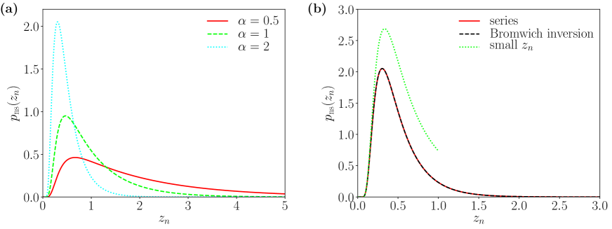
Figure 1: (a) The function $p_{ns}(z_{n})$ for evaluated using the representation Eq. (45) by taking into account the zeros of $J_{\alpha-1}(u)$ on $(0,1000]$. Shown are the function for $\alpha=1/2$ (solid line), $\alpha=1$ (dashed line) and $\alpha=2$ (dotted line). (b) The function $p_{ns}(z_{n})$ for $\alpha=2$, evaluated using the representation Eq. (45) by taking into account the zeros of $J_{\alpha-1}(u)$ on $(0,1000]$ (solid line) compared with numerical computation of the Bromwich inversion formula Eq. (44) (dashed line), the two curves are indistinguishable. Also shown is the analytic prediction for the behavior at small $z_{n}$ given by Eq. (49) (dotted line). Note that $\epsilon=1$, without loss of generality.

The inverse Laplace transform in Eq. (44) can also be evaluated numerically, for instance using the numerical integration option of Mathematica, this turns out to be relatively simple to do and in Fig. 1(b) we show the results for $\alpha=2$ from the infinite series representation Eq. (45) (again using the zeros of $J_{\alpha-1}(u)$ on $(0,1000]$) compared with the numerical inversion of the Laplace transform. We see that the agreement is perfect, however in both cases numerical precision becomes an issue for small $z_{n}$ due to the presence of the essential singularity exhibited in Eq. (49). The asymptotic expression for small $z_{n}$ Eq. (49) is also shown, we see that while it predicts the position of the maximum of the probability density function it over estimates its height. Of course, on approaching $z_{n}=0$ the agreement is perfect.

The joint probability distribution for $(x,y,z_{n})$ is more difficult to analyze. However we may again examine the form of the distribution for small $z_{n}$ using the asymptotic behavior given in Eq. (39) for large $s$ which leads to

$$p_{ns}(x,y,z_{n})=\frac{\epsilon^{\alpha+1}}{\pi\alpha\Gamma(\alpha)z_{n}^{\alpha+2}}\left(1+\frac{\rho^{2}}{4\alpha}\right)^{\alpha+\frac{3}{2}}\exp\left[-\frac{\epsilon}{z_{n}}\left(1+\frac{\rho^{2}}{4\alpha}\right)^{2}\right],$$ (50)

where $\rho=\sqrt{x^{2}+y^{2}}$.

The steady state current corresponding to the processes $x,y$ and $z_{n}$ is given by

$${\bf J}_{ns}(x,y,z_{n})=-\left[\frac{\partial p_{ns}}{\partial x}(x,y,z_{n})+xp_{ns}(x,y,z_{n})\right]{\bf e}_{x}-\left[\frac{\partial p_{ns}}{\partial y}(x,y,z_{n})+yp_{ns}(x,y,z_{n})\right]{\bf e}_{y}$$

$$+\eta\left[\left(\frac{\epsilon\eta}{4}(x^{2}+y^{2})-z_{n}\right)p_{ns}(x,y,z_{n})\right]{\bf e}_{z},$$ (51)

and using the rotational symmetry of the problem we can write this as

$${\bf J}_{ns}(\rho,z_{n})=p_{ns}(\rho,z_{n})\left[-\left(\frac{\partial\ln p_{ns}}{\partial\rho}(\rho,z_{n})+\rho\right){\bf e}_{\rho}+\frac{2}{\alpha}\left(\frac{\epsilon}{2\alpha}\rho^{2}-z_{n}\right){\bf e}_{z}\right]$$ (52)

where ${\bf e}_{\rho}=(x{\bf e}_{x}+y{\bf e}_{y})/\rho$ is the polar basis vector and we recall that $\eta=2/\alpha$. In the region where $z_{n}\ll 1$ we can then use the asymptotic result Eq. (50) to find

$${\bf J}_{ns}(\rho,z_{n}) \simeq \frac{\rho\epsilon^{\alpha+2}}{\pi\alpha^{2}\Gamma(\alpha)z_{n}^{\alpha+2}}\left(1+\frac{\rho^{2}}{4\alpha}\right)^{\alpha+\frac{3}{2}}\exp\left[-\frac{1}{z_{n}}\left(1+\frac{\rho^{2}}{4\alpha}\right)^{2}\right]\left[\frac{1}{z_{n}}\left(1+\frac{\rho^{2}}{4\alpha}\right){\bf e}_{\rho}+\frac{1}{\alpha}\rho{\bf e}_{z}\right].$$ (53)

We will see in what follows that the full steady state distribution for the process $(x,y,z)=(x,y,z_{n}+z_{o})$ as well as the corresponding current is simply related to the corresponding results for $(x,y,z_{n})$. However as we cannot obtain a fully analytical form for the distribution of the latter we must resort to a perturbative analysis.

III.2 Numerical results for the process $(x,y,z_{n})$

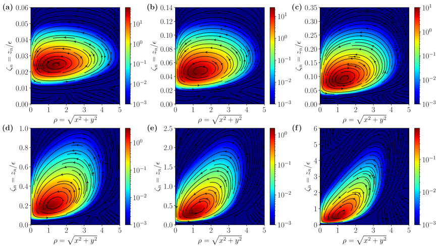
Figure 2: The probability distribution $p_{cns1}(\rho,\zeta_{n})$ for the process $(\rho,\zeta_{n})$ along with the associated current lines for various values of $\eta=2/\alpha$: (a) $\eta=0.05$, (b) $\eta=0.1$, (c) $\eta=0.2$, (d) $\eta=0.5$, (e) $\eta=1$, and (f) $\eta=2$. In all cases there is a single vortex. These results were obtained by integrating numerically the steady state Fokker-Planck equation for $(\rho,\zeta_{n})$ with the finite element method.

The most straightforward way to determine the steady state distribution of the process $(x,y,z_{n})$ is to solve the time independent Fokker-Planck equation for the process in the case where we set $\epsilon=1$ to numerically evaluate what we denote by $p_{ns1}(x,y,z_{n})$. The distribution for general $\epsilon$ is then simply obtained via

$$p_{ns}(x,y,z_{n})=\epsilon p_{ns1}(x,y,\epsilon z_{n}).$$ (54)

We thus solve the steady state diffusion equation using the current given by Eq. (51). Given the essential singularity at $z_{n}=0$ the numerical resolution is difficult in this region, however this problem can be surmounted by adding a small diffusive component to the process $z_{n}$. In our computations a diffusion constant of $10^{-6}$ was taken. This is equivalent to numerically solving the steady state Fokker-Planck equation for $\epsilon=1000$ and then extracting the probability density function for $\zeta_{n}=z_{n}/\epsilon$. In this analysis the only parameter corresponds to $\alpha=2/\eta$. Shown in Fig. 2 is the stationary probability density for the cylindrical coordinate process $(\rho,\zeta_{n})$, denoted by $p_{cns1}$ and which is simply related to $p_{ns1}$ via

$$p_{cns1}(\rho,\zeta_{n})=2\pi\rho p_{ns1}(\rho,\zeta_{n}),$$ (55)

for several values of $\eta$. On the same figure we also the associated current as a function of $\zeta_{n}$ and the radial coordinate $\rho$. We see that in all cases there is a single current vortex which is located close to the maximum of the probability density function $p_{cns1}(\rho,\zeta_{n})$.

III.3 Distribution for the full model

In the previous analysis we did not include the OU contribution to the movement in the $z$ direction. If we denote full distribution $p_{fs}(x,y,z)$ we see that its two sided Laplace transform with respect to $z$ is given by

$$\tilde{p}_{fs}(x,y,s)=\tilde{p}_{ns}(x,y,s)\exp\left(\frac{s^{2}}{2}\right)=\frac{(s\epsilon)^{\frac{\alpha}{2}}}{2\pi\alpha\Gamma(\alpha)I_{\alpha}(2\sqrt{s\epsilon})}\exp\left(\frac{s^{2}}{2}\right)\exp\left[-\frac{\sqrt{s\epsilon}}{2\alpha}\frac{I_{\alpha-1}(2\sqrt{s\epsilon})}{I_{\alpha}(2\sqrt{s\epsilon})}(x^{2}+y^{2})\right].$$ (56)

Note that we take the two sided Laplace transform as the total process $z$ is can now become negative.

The full marginal distribution for $z$ can obviously be derived from the convolution with the pdf of the OU component of the $z$ motion, that is to say

$$p_{fs}(z)=\frac{1}{\sqrt{2\pi}}\int_{0}^{\infty}dz_{n}\exp\left[-\frac{1}{2}(z-z_{n})^{2}\right]p_{ns}(z_{n}).$$ (57)

However, to make the link with previous studies at the perturbative level, of the effect of the non-conservative force on the steady state distribution we now proceed by expanding Eq. (56) in $\epsilon$. We find that the form of this expansion is

$$\tilde{p}_{fs}(\rho,s)=\frac{1}{2\pi}\exp\left(\frac{s^{2}-\rho^{2}}{2}\right)\sum_{k=0}^{\infty}\epsilon^{k}s^{k}C_{k}(\rho,\alpha),$$ (58)

where we again emphasize that $p_{fs}$ is still the probability density function for $(x,y,z)$ but we have written it as a function of $(\rho,z)$ for compactness. Carrying out the above expansion explicitly, we find the first three terms:

$$C_{0}(\rho,\alpha) =1$$ (59)

$$C_{1}(\rho,\alpha) =-\frac{2\alpha+\rho^{2}}{2\alpha(\alpha+1)}$$ (60)

$$C_{2}(\rho,\alpha) =\frac{4\alpha^{2}(3+\alpha)+4\alpha(3+\alpha)\rho^{2}+(2+\alpha)\rho^{4}}{8\alpha^{2}(1+\alpha)^{2}(2+\alpha)}$$ (61)

$$C_{3}(\rho,\alpha) =-\frac{(8\alpha^{3}+12\alpha^{2}\rho^{2})(\alpha^{2}+8\alpha+19)+6\alpha(\alpha+3)(\alpha+4)\rho^{4}+(\alpha+2)(\alpha+3)\rho^{6}}{48\alpha^{3}(\alpha+1)^{3}(\alpha+2)(\alpha+3)}.$$ (62)

We can formally invert the Laplace transform in Eq. (58) to obtain

$$p_{fs}(\rho,z)=\frac{\exp\left(-\frac{\rho^{2}}{2}\right)}{(2\pi)^{\frac{3}{2}}}\sum_{k=0}^{\infty}\epsilon^{k}C_{k}(\rho,\alpha)\frac{\partial^{k}}{\partial z^{k}}\exp\left(-\frac{z^{2}}{2}\right).$$ (63)

We find that to order $\epsilon^{3}$

$$p_{fs}(\rho,z) =\frac{\exp\left(-\frac{\rho^{2}+z^{2}}{2}\right)}{(2\pi)^{\frac{3}{2}}}\left[1+\epsilon z\frac{2\alpha+\rho^{2}}{2\alpha(\alpha+1)}+\epsilon^{2}(z^{2}-1)\frac{4\alpha^{2}(3+\alpha)+4\alpha(3+\alpha)\rho^{2}+(2+\alpha)\rho^{4}}{8\alpha^{2}(1+\alpha)^{2}(2+\alpha)}\right.$$

$$+\left.\epsilon^{3}z(z^{2}-3)\frac{(8\alpha^{3}+12\alpha^{2}\rho^{2})(\alpha^{2}+8\alpha+19)+6\alpha(\alpha+3)(\alpha+4)\rho^{4}+(\alpha+2)(\alpha+3)\rho^{6}}{48\alpha^{3}(\alpha+1)^{3}(\alpha+2)(\alpha+3)}\right].$$ (64)

One can verify that the expansion to first order in $\epsilon$ agrees with the first order perturbation computations of Refs. moyses2015 ; mangeat2019 . It can be extended to arbitrarily higher orders. The first terms $k=1,\ 2$ and $3$ of the series (63) are represented in Fig. 3 (up to a factor $2\pi\rho$ to switch to cylindrical coordinates) for $\alpha=10$ (corresponding to a typical experimental value $\eta=0.2$). The first order correction exhibits a local maximum above $z=0$ and local minimum below. The second order term has a minimum on the axis $z=0$ and two maxima above and below. The third order result exhibits two maxima and two minima. This generation of maxima and minima is due to the generation of nodes in the functions

$$V_{k}(z)=\frac{\partial^{k}}{\partial z^{k}}\exp\left(-\frac{z^{2}}{2}\right).$$ (65)

which are related to the Hermite polynomials associated with the simple Harmonic oscillator.

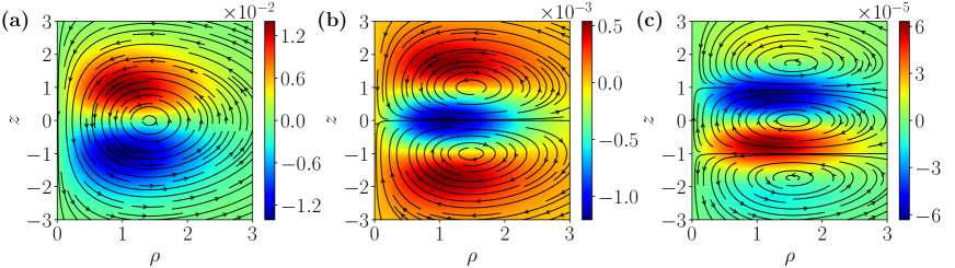
Figure 3: The perturbative corrections to third order in $\epsilon$ of the density in cylindrical coordinates $p_{fsc}=2\pi\rho p_{fs}=\sum_{k}p_{fsc}^{(k)}\epsilon^{k}$ and the associated current lines for the case $\alpha=10$ (corresponding to $\eta=0.2$). (a) $p^{(1)}_{fsc}(\rho,z),\ {\bf J}^{(1)}_{fs}(\rho,z)$. (b) $p^{(2)}_{fsc}(\rho,z),\ {\bf J}^{(2)}_{fs}(\rho,z)$. (c) $p^{(3)}_{fsc}(\rho,z),\ {\bf J}^{(3)}_{fs}(\rho,z)$.

III.4 Steady state currents

One of the key points of interest in the model here is the presence of currents which are the signature of the breaking of time reversal symmetry in the non-equilibrium steady state. The current is explicitly given by

$${\bf J}_{f}(\rho,z)=-\left[\frac{\partial p_{fs}}{\partial\rho}(\rho,z)+\rho p_{fs}(\rho,z)\right]{\bf e}_{\rho}+\frac{2}{\alpha}\left[\left(\frac{\epsilon}{2\alpha}\rho^{2}-z\right)p_{fs}(\rho,z)-\frac{\partial p_{fs}}{\partial z}(\rho,z)\right]{\bf e}_{z}.$$ (66)

To examine the current in the steady state it is again convenient to work with the two sided Laplace transform of the current

$$\tilde{\bf J}_{fs}(x,y,s)=\int dz\exp(-sz)\ {\bf J}_{fs}(x,y,z),$$ (67)

and from this we find

$$\tilde{\bf J}_{fs}(x,y,s) =-\left[\frac{\partial\tilde{p}_{fs}}{\partial x}(x,y,s)+x\tilde{p}_{fs}(x,y,s)\right]{\bf e}_{x}-\left[\frac{\partial\tilde{p}_{fs}}{\partial y}(x,y,s)+y\tilde{p}_{fs}(x,y,s)\right]{\bf e}_{y}$$

$$+\eta\left[\frac{\epsilon\eta}{4}(x^{2}+y^{2})\tilde{p}_{fs}(x,y,z)+\frac{\partial\tilde{p}_{fs}}{\partial s}(x,y,s)-s\tilde{p}_{fs}(x,y,s)\right]{\bf e}_{z}.$$ (68)

It is convenient to write this in terms of the functions $A(s)$ and $B(s)$ in Eq. (27) and (28)

$$\tilde{\bf J}_{fs}(x,y,s)={\tilde{p}_{fs}(x,y,s)}\left\{-[1-A(s)](x{\bf e}_{x}+y{\bf e}_{y})+\eta\left[\left(\frac{\epsilon\eta}{4}-\frac{A^{\prime}(s)}{2}\right)(x^{2}+y^{2})+2\frac{B^{\prime}(s)}{B(s)}\right]{\bf e}_{z}\right\}.$$ (69)

An interesting consequence of this result is that the current for the full system, taking into account the term $z_{o}$, is related to that of the system $(x,y,z_{n})$ by a simple convolution in the same way as the probability density functions are related, that is to say

$${\bf J}_{fs}(x,y,z)=\frac{1}{\sqrt{2\pi}}\int_{0}^{\infty}dz_{n}\exp\left[-\frac{1}{2}(z-z_{n})^{2}\right]{\bf J}_{ns}(x,y,z_{n}).$$ (70)

We thus see that both the steady state distribution and current of the full process $(x,y,z)$ is related to the process $(x,y,z_{n})$ by a simple convolution.

We proceed by using the representation Eq. (63) to express the current as a power series in $\epsilon$

$${\bf J}_{fs}(\rho,z)=\sum_{k=0}^{\infty}\epsilon^{k}{\bf J}^{(k)}_{fs}(\rho,z),$$ (71)

where we have

$${\bf J}^{(k)}_{fs}(\rho,z)=\frac{\exp\left(-\frac{\rho^{2}}{2}\right)}{(2\pi)^{\frac{3}{2}}}\left\{-\frac{\partial C_{k}}{\partial\rho}(\rho,\alpha)V_{k}(z){\bf e}_{\rho}+\left[\frac{\rho^{2}}{\alpha^{2}}C_{k-1}(\rho,\alpha)V_{k-1}(z)-\frac{2}{\alpha}C_{k}(\rho,\alpha)(V^{\prime}_{k}(z)+zV_{k}(z))\right]{\bf e}_{z}\right\}.$$ (72)

It is obvious that $V^{\prime}_{k}(z)=V_{k+1}(z)$ and a straight forward exercise shows that

$$zV_{k}(z)=-V_{k+1}(z)-kV_{k-1}(z).$$ (73)

Using this we find

$${\bf J}^{(k)}_{fs}(\rho,z)=\frac{\exp\left(-\frac{\rho^{2}}{2}\right)}{(2\pi)^{\frac{3}{2}}}\left\{-\frac{\partial C_{k}}{\partial\rho}(\rho,\alpha)V_{k}(z){\bf e}_{\rho}+V_{k-1}(z)\left[\frac{\rho^{2}}{\alpha^{2}}C_{k-1}(\rho,\alpha)+\frac{2k}{\alpha}C_{k}(\rho,\alpha)\right]{\bf e}_{z}\right\}.$$ (74)

The divergence of the steady state current must be zero and this must hold at each order in the expansion in $\epsilon$, we thus obtain $\nabla\cdot{\bf J}^{(k)}_{fs}=0$ for all $k$ which yields differential equations relating the polynomials $C_{k}(\rho,\alpha)$ which can be used to generate them iteratively starting at $C_{0}(\rho,\alpha)=1$.

The first three orders in perturbation theory for the current then give

$${\bf J}^{(1)}_{fs}(\rho,z) =\frac{\exp\left(-\frac{\rho^{2}+z^{2}}{2}\right)}{(2\pi)^{\frac{3}{2}}}\left[-\frac{\rho z}{\alpha(\alpha+1)}{\bf e}_{\rho}+\frac{\rho^{2}-2}{\alpha(\alpha+1)}{\bf e}_{z}\right]$$ (75)

$${\bf J}^{(2)}_{fs}(\rho,z) =\frac{\exp\left(-\frac{\rho^{2}+z^{2}}{2}\right)}{(2\pi)^{\frac{3}{2}}}\left[-\frac{\rho\left(z^{2}-1\right)\left[(\alpha+2)\rho^{2}+2\alpha(\alpha+3)\right]}{2\alpha^{2}(\alpha+1)^{2}(\alpha+2)}{\bf e}_{\rho}\right.$$

$$+\left.\frac{z\left[(\alpha+2)\rho^{4}+2\left(\alpha^{2}+\alpha-4\right)\rho^{2}-4\alpha(\alpha+3)\right]}{2\alpha^{2}(\alpha+1)^{2}(\alpha+2)}{\bf e}_{z}\right]$$ (76)

$${\bf J}^{(3)}_{fs}(\rho,z) =\frac{\exp\left(-\frac{\rho^{2}+z^{2}}{2}\right)}{(2\pi)^{\frac{3}{2}}}\left[-\frac{\rho z\left(z^{2}-3\right)\left[(\alpha+2)(\alpha+3)\rho^{4}+4\alpha(\alpha+3)(\alpha+4)\rho^{2}+4\alpha^{2}(\alpha^{2}+8\alpha+19)\right]}{8\alpha^{3}(\alpha+1)^{3}(\alpha+2)(\alpha+3)}{\bf e}_{\rho}\right.$$

$$+\left.\frac{\left(z^{2}-1\right)\left[(\alpha+2)(\alpha+3)\rho^{6}+2(\alpha+3)(2\alpha^{2}+5\alpha-6)\rho^{4}+4\alpha(\alpha^{3}+4\alpha^{2}-9\alpha-48)\rho^{2}-8\alpha^{2}(\alpha^{2}+8\alpha+19)\right]}{8\alpha^{3}(\alpha+1)^{3}(\alpha+2)(\alpha+3)}{\bf e}_{z}\right]$$ (77)

One can again verify that the expansion to first order in $\epsilon$ agrees with the first order perturbation computations of Refs. moyses2015 ; mangeat2019 .

The first three perturbative corrections to the steady state current are shown in Fig. 3 for the case $\alpha=10$ superimposed on the corresponding corrections to the steady state probability density function of $\rho$ and $z$. We see that the first order correction possesses and single vortex, while the second and third order corrections have two and three vortices respectively. A thorough numerical investigation however rules out the existence of more than one vortex and when fully summed the vortices seen in the individual terms of the perturbation almost certainly vanish. Indeed it seems physically unlikely that a tracer current circulates around more that one central vortex. When $\rho$ is large, particles are pushed upwards by the non-conservative force and when it becomes small enough the harmonic restoring term pulls them down.

III.5 The circulation of the current

Of particular interest is the circulation of the non-equilibrium current defined by

$$\Omega_{fs}=\frac{1}{2\pi}\int d{\bf x}\ \nabla\times{\bf J}_{fs}({\bf x})\cdot{\bf e}_{\phi}$$ (78)

where ${\bf e}_{\phi}=(-y{\bf e}_{x}+x{\bf e}_{y})/\rho$ is the basis vector of the polar angle $\phi$, and by symmetry the local current circulates around this direction. Here is we use Eq. (69) for steady state current written in polar coordinates

$$\tilde{\bf J}_{fs}(\rho,s)={\rho\tilde{p}_{fs}(\rho,s)}\left\{-[1-A(s)]{\bf e}_{\rho}+\eta\left[\left(\frac{\epsilon\eta}{4}-\frac{A^{\prime}(s)}{2}\right)\rho^{2}+2\frac{B^{\prime}(s)}{B(s)}\right]{\bf e}_{z}\right\},$$ (79)

which yields

$$\Omega_{fs}=\int dz\rho d\rho\left[\frac{\partial}{\partial z}J_{fs,\rho}-\frac{\partial}{\partial\rho}J_{fs,z}\right]=\int d\rho\tilde{J}_{fs,z}(\rho,0).$$ (80)

In the above we have used that the first term in the integrand integrates directly giving zero and the second term has been integrated by parts. Using the explicit form of ${\bf J}_{fs}$ in Eq. (79) together with Eqs. (37), (36), (39), we obtain

$$\Omega_{fs}=-\frac{\eta^{2}\epsilon}{4\sqrt{2\pi}(\eta+2)}.$$ (81)

Interestingly this is in agreement, up to a change in sign as we have reversed the direction of propagation of the laser here, with the first order perturbation calculation of the circulation given in Ref. moyses2015 . The first order perturbative result of Ref. moyses2015 thus turns out to be exact for all values of $\epsilon$.

IV Conclusions

In this paper we have analyzed the simplest model used for optical traps that takes into account non-conservative forces generated by the laser interaction with the trapped particle’s dipole moment. Non-conservative forces occur frequently in physics, notably due to the magnetic components of electromagnetic fields, however analytical descriptions of the associated steady states are very rare and no general theory exists. We were able to find exact results for the Laplace transform with respect to the coordinate $z$ (the direction of laser propagation) of the full non-equilibrium steady state probability distribution. In the limit $\varepsilon=\infty$, $z$ can be replaced by the non-conservative part $z_{n}$. We have also computed the Laplace transform of the marginal distribution of the nonconservative part of the displacement in $z$, this can be formally inverted and the full distribution found. The full distribution of $z$ is then simply related to this latter distribution via a convolution with a Gaussian. Interestingly the same convolution relationship is found to hold for the currents. The Laplace transform representation of the full three dimensional probability distribution can be used to develop a systematic perturbation theory of the full steady state probability distribution as a series in the magnitude of the non-equilibrium force, which here is denoted by $\epsilon$. In this paper we have given explicit results to ${\cal O}(\epsilon^{3})$, extending the first order results of moyses2015 ; mangeat2019 , but arbitrary higher orders can be deduced from our formalism. Using our results, we were also able to compute the circulation of the current in the steady states, interestingly this exact results agrees with that of first order perturbation theory found in moyses2015 .

In mangeat2019 the same model but with under damped dynamics was studied. The presence of non-conservative forces means that the steady state depends on the friction in the system and the velocity and spatial degrees of freedom are not independent as is the case with the equilibrium Gibbs-Boltzmann distribution. The results of mangeat2019 were perturbative and it would be interesting to see if the method used here could be used to exactly analyze the underdamped model.

V Acknowledgements

M.M. was partially financially supported by the German Research Foundation (DFG) within the Collaborative Research Center SFB 1027.

References

- (1) A. Ashkin, Acceleration and Trapping of Particles by Radiation Pressure, Phys. Rev. Lett. 24, 156-159 (1970).
- (2) A. Ashkin, Summary of the First Decade’s Work on Optical Trapping and Manipulation of Particles in Optical Trapping and Manipulation of Neutral Particles Using Lasers, World Scientific (2006).
- (3) A. Ashkin and J. M. Dziedzic, Optical trapping and manipulation of viruses and bacteria, Science 235, 1517-1520 (1987).
- (4) D. G. Grier, Optical tweezers in colloid and interface science, Current Opinion in Colloid & Interface Science 2, 264-270 (1997).
- (5) B. Lukic, S. Jeney, Z. Sviben, A. J. Kulik, E.-L. Florin, and L. Forro, Motion of a colloidal particle in an optical trap, Phys. Rev. E 76, 011112 (2007).
- (6) P. Jop, J. R. Gomez-Solano, A. Petrosyan, and S. Ciliberto, Experimental study of out-of-equilibrium fluctuations in a colloidal suspension of Laponite using optical traps, J. Stat. Mech. 2009, P04012 (2009).
- (7) M. Dienerowitz, M. Mazilu, and K. Dholakia, Optical manipulation of nanoparticles: a review, JNP 2, 021875 (2008).
- (8) J. Gieseler, B. Deutsch, R. Quidant, and L. Novotny, Subkelvin Parametric Feedback Cooling of a Laser-Trapped Nanoparticle, Phys. Rev. Lett. 109, 103603 (2012).
- (9) T. Li, M. G. Raizen, Brownian motion at short time scales, Annalen der Physik 525, 281 (2013).
- (10) J. Bateman, S. Nimmrichter, K. Hornberger, and H. Ulbricht, Near-field interferometry of a free-falling nanoparticle from a point-like source, Nat. Comm. 5, 4788 (2014).
- (11) A. Lehmuskero, P. Johansson, H. Rubinsztein-Dunlop, L. Tong, and M. Käll, Laser Trapping of Colloidal Metal Nanoparticles, ACS Nano 9, 3453-3469 (2015).
- (12) S. Wildermuth, P. Krüger, C. Becker, M. Brajdic, S. Haupt, A. Kasper, R. Folman, and J. Schmiedmayer, Optimized magneto-optical trap for experiments with ultracold atoms near surfaces, Phys. Rev. A 69, 030901 (2004).
- (13) S. Chu, Laser Manipulation of Atoms and Particles, Science 253, 861-866 (1991).
- (14) M. D. Wang, H. Yin, R. Landick, J. Gelles, and S. M. Block, Stretching DNA with optical tweezers, Biophysical J. 72, 1335-1346 (1997).
- (15) C. Bustamante, S. B. Smith, J. Liphardt, and D. Smith, Single-molecule studies of DNA mechanics, Current Opinion in Structural Biology 3, 279-285 (2000).
- (16) J. M. Huguet, C. Bizarro, N. Forns, S. B. Smith, C. Bustamante, and F. Ritort, Single-molecule derivation of salt dependent base-pair free energies in DNA, PNAS 107, 15431-15436 (2010).
- (17) J.-D. Wen, M. Manosas, P. T. X. Li, S. B. Smith, C. Bustamante, F. Ritort, and I. Tinoco , Force Unfolding Kinetics of RNA Using Optical Tweezers. I. Effects of Experimental Variables on Measured Results, Biophysical J. 92, 2996-3009 (2007).
- (18) F. Ritort, S. Mihardja, S. B. Smith, and C. Bustamante, Condensation Transition in DNA-Polyaminoamide Dendrimer Fibers Studied Using Optical Tweezers, Phys. Rev. Lett. 96, 118301 (2006).
- (19) D. C. Moore, A. D. Rider, and G. Gratta, Search for Millicharged Particles Using Optically Levitated Microspheres, Phys. Rev. Lett. 113, 251801 (2014).
- (20) G. Ranjit, M. Cunningham, K. Casey, and A. A. Geraci, Zeptonewton force sensing with nanospheres in an optical lattice, Phys. Rev. A 93, 053801 (2016).
- (21) J. Liu and K.-D. Zhu, Nanogravity gradiometer based on a sharp optical nonlinearity in a levitated particle optomechanical system, Phys. Rev. D 95, 044014 (2017).
- (22) A. Arvanitaki and A. A. Geraci, Detecting High-Frequency Gravitational Waves with Optically Levitated Sensors, Phys. Rev. Lett. 110, 071105 (2013).
- (23) A. D. Rider, D. C. Moore, C. P. Blakemore, M. Louis, M. Lu, and G. Gratta, Search for Screened Interactions Associated with Dark Energy below the 100 µm Length Scale, Phys. Rev. Lett. 117, 101101 (2016).
- (24) D. Collin, F. Ritort, C. Jarzynski, S. B. Smith, I. Tinoco Jr, and C. Bustamante, Verification of the Crooks fluctuation theorem and recovery of RNA folding free energies, Nature 437, 7056 (2005).
- (25) D. M. Carberry, J. C. Reid, G. M. Wang, E. M. Sevick, D. J. Searles, and D. J. Evans, Fluctuations and Irreversibility: An Experimental Demonstration of a Second-Law-Like Theorem Using a Colloidal Particle Held in an Optical Trap, Phys. Rev. Lett. 92, 140601 (2004).
- (26) D. M. Carberry, M. A. B Baker, G. M. Wang, E. M. Sevick, and D. J. Evans, An optical trap experiment to demonstrate fluctuation theorems in viscoelastic media, J. Opt. A: Pure Appl. Opt. 9, 5204 (2007).
- (27) A. Bérut, A. Imparato, A. Petrosyan, and S. Ciliberto, Stationary and Transient Fluctuation Theorems for Effective Heat Fluxes between Hydrodynamically Coupled Particles in Optical Traps, Phys. Rev. Lett. 116, 068301 (2016).
- (28) A. Bassi, K. Lochan, S. Satin, T. P. Singh, and H. Ulbricht, Models of wave-function collapse, underlying theories, and experimental tests, Rev. Mod. Phys. 85, 471-527 (2013).
- (29) P. Wu, R. Huang, C. Tischer, A. Jonas, and E.-L. Florin, Direct Measurement of the Nonconservative Force Field Generated by Optical Tweezers, Phys. Rev. Lett. 103, 108101 (2009).
- (30) Y. Roichmann, B. Sun, A. Stolarski, and D. G. Grier, Influence of Nonconservative Optical Forces on the Dynamics of Optically Trapped Colloidal Spheres: The Fountain of Probability, Phys. Rev. Lett. 101, 128301 (2008).
- (31) B. Sun, J. Lin, E. Darby, A. Y. Grosberg, and D. G. Grier, Brownian vortexes, Phys. Rev. E 80, 010401 (2009).
- (32) B. Sun, D. G. Grier, and A. Y. Grosberg, Minimal model for Brownian vortexes, Phys. Rev. E 82, 021123 (2010).
- (33) S. H. Simpson and S. Hanna, First-order nonconservative motion of optically trapped nonspherical particles, Phys. Rev. E 82, 031141 (2010).
- (34) H. W. Moyses, R. O. Bauer, A. Y. Grosberg, and D. G. Grier, Perturbative theory for Brownian vortexes, Phys. Rev. E 91, 062144 (2015).
- (35) M. de Messieres, N. A. Denesyuk, and A. La Porta, Noise associated with nonconservative forces in optical traps, Phys. Rev. E 84, 031108 (2011).
- (36) Y. Amarouchene, M. Mangeat, B. V. Montes, L. Ondic, T. Guérin, D. S. Dean, and Y. Louyer, Nonequilibrium Dynamics Induced by Scattering Forces for Optically Trapped Nanoparticles in Strongly Inertial Regimes, Phys. Rev. Lett. 122, 183901 (2019).
- (37) M. Mangeat, Y. Amarouchene, Y. Louyer, T. Guérin, and D. S. Dean, Role of nonconservative scattering forces and damping on Brownian particles in optical traps, Phys. Rev. E 99, 052107 (2019).
- (38) T. B. Liverpool, Steady-state distributions and nonsteady dynamics in nonequilibrium systems, Phys. Rev. E 101, 042107 (2021).
- (39) J. Gieseler, L. Novotny, and R. Quidant, Thermal nonlinearities in a nanomechanical oscillator, Nat. Phys. 9, 806 (2013).
- (40) D. Boyer and D. S. Dean, On the distribution of estimators of diffusion constants for Brownian motion, J. Phys. A: Math. Theor. 44, 335003 (2011).
- (41) M. Abramowitz and I. A. Stegun, Handbook of Mathematical Tables, (Dover, New York, 1965).
- (42) I. Colombaro, A. Giusti and F. Mainardi, A class of linear viscoelastic models based on Bessel functions, Meccanica 52, 825 (2017).
- (43) J. T. Kent, Some probabilistic properties of Bessel functions, Ann. Probab. 6,760 (1978).
- (44) R. K. Getoor and M. J. Sharpe, Excursions of Brownian motion and Bessel processes, Z. Wahr. Ver. Gebiete 47, 83 (1979).