Late-transition vs smooth deformation models
for the resolution of the Hubble crisis
Abstract
Gravitational transitions at low redshifts () have been recently proposed as a solution to the Hubble and growth tensions. Such transitions would naturally lead to a transition in the absolute magnitude of type Ia supernovae (SnIa) at (Late Transitions - ) and possibly in the dark energy equation of state parameter (Late Transitions - ). Here, we compare the quality of fit of this class of models to cosmological data, with the corresponding quality of fit of the cosmological constant model (CDM) and some of the best smooth deformation models (CDM, CPL, PEDE). We also perform model selection via the Akaike Information Criterion and the Bayes factor. We use the full CMB temperature anisotropy spectrum data, the baryon acoustic oscillations (BAO) data, the Pantheon SnIa data, the SnIa absolute magnitude as determined by Cepheid calibrators and the value of the Hubble constant as determined by local SnIa calibrated using Cepheids. We find that smooth deformation models perform worse than transition models for the following reasons: 1) They have a worse fit to low- geometric probes (BAO and SnIa data); 2) They favor values of the SnIa absolute magnitude that are lower as compared to the value obtained with local Cepheid calibrators at ; 3) They tend to worsen the growth tension. We also find that the transition model () does not provide a better quality of fit to cosmological data than a pure transition model () where is fixed to the CDM value at all redshifts. We conclude that the model has significant statistical advantages over smooth late-time deformation models in addressing the Hubble crisis.
I Introduction
The scenario considered as the standard model in cosmology is the cosmological constant and cold dark matter (CDM) model, hereafter denoted as CDM, as it is remarkably successful in fitting cosmological and astrophysical observations on a vast range of scales. However, this scenario is not a first principles theory, and it is based on unknown quantities (dark matter, dark energy and inflation), therefore can be considered as a low energy and large scales approximation to a physical law, which has yet to be discovered. In this context, the observational problems in the estimates of the main cosmological parameters, see Refs. Di Valentino et al. (2021a, b, c, d), can hint towards the presence of deviations from the CDM scenario Perivolaropoulos and Skara (2021a); Saridakis et al. (2021).
In particular, the most statistically significant inconsistency is the well known Hubble constant tension, currently above the level (see Verde et al. (2019); Riess (2019); Di Valentino (2021); Di Valentino et al. (2021e); Perivolaropoulos and Skara (2021a); Shah et al. (2021) and references therein). This tension refers to the disagreement between the value of estimated from the Planck satellite data Aghanim et al. (2020a), assuming a CDM model, and the measured by the SH0ES collaboration Riess et al. (2021a). However, there are many ways to obtain the Hubble constant value, and most of the early indirect estimates agree with Planck, as the Cosmic Microwave Background (CMB) ground telescopes Aiola et al. (2020); Dutcher et al. (2021) or the Baryon Acoustic Oscillations (BAO) measurements Alam et al. (2021), while most of the late time measurements agree with SH0ES, even if obtained with different teams, methods or geometric calibrators Soltis et al. (2021); Pesce et al. (2020); Kourkchi et al. (2020); Schombert et al. (2020); Blakeslee et al. (2021). Finally, there are a few measurements that are in agreement with both sides, as the Tip of the Red Giant Branch Freedman (2021), even if the re-analysis of Anand et al. (2021) shows a better consistency with the SH0ES value, or those based on the time delay Birrer et al. (2020).
An additional challenge for the standard model is the growth tension. Dynamical cosmological probes favor weaker growth of perturbations than geometric probes in the context of general relativity and the Planck18/CDM standard model at a level of about Hildebrandt et al. (2017); Nesseris et al. (2017); Macaulay et al. (2013); Kazantzidis and Perivolaropoulos (2018); Skara and Perivolaropoulos (2020); Kazantzidis and Perivolaropoulos (2019); Perivolaropoulos and Kazantzidis (2019). It would therefore be of particular interest to construct theoretical models that have the potential to simultaneously address both the and growth tensions.
A wide range of theoretical models have been proposed as possible resolutions of the Hubble tension (Di Valentino et al., 2021e; Kazantzidis and Perivolaropoulos, 2019). They can be divided in three broad classes:
-
•
“Early time” models that recalibrate the scale of the sound horizon at recombination by modifying physics during the pre-recombination epoch. These models deform the Hubble expansion rate before recombination at by introducing early dark energy (Karwal and Kamionkowski, 2016; Poulin et al., 2019; Sakstein and Trodden, 2020; Niedermann and Sloth, 2021; Hill et al., 2020; Murgia et al., 2021; D’Amico et al., 2021; Gogoi et al., 2021; Chudaykin et al., 2021, 2020; Agrawal et al., 2019; Niedermann and Sloth, 2020; Ye and Piao, 2020; Lin et al., 2019; Braglia et al., 2020; Hill et al., 2021; Chang, 2021; Ye et al., 2021; Gómez-Valent et al., 2021; Jiang and Piao, 2021; Karwal et al., 2021; Poulin et al., 2021), extra neutrinos or relativistic species at recombination (Vagnozzi, 2020; Seto and Toda, 2021; Carneiro et al., 2019; Gelmini et al., 2021, 2020; D’Eramo et al., 2018; Pandey et al., 2020; Xiao et al., 2020; Nygaard et al., 2021; Blinov et al., 2020; Binder et al., 2018; Choi et al., 2020; Di Valentino et al., 2018; Escudero and Witte, 2020; Arias-Aragon et al., 2021; Blinov and Marques-Tavares, 2020; Flambaum and Samsonov, 2019; Anchordoqui et al., 2021; Das, 2021; Fernandez-Martinez et al., 2021; Feng et al., 2021; Ghosh et al., 2021), features in the primordial power spectrum Hazra et al. (2019); Keeley et al. (2020), or evaporatig primordial black holes Nesseris et al. (2020) etc. These models however, can alleviate but not fully solve the Hubble tension Arendse et al. (2020); Lin et al. (2021); Schöneberg et al. (2021), and they tend to predict stronger growth of perturbations than implied by dynamical probes like redshift space distortion (RSD) and weak lensing (WL) data and thus they worsen the growth tension (Jedamzik et al., 2020). This issue however is still under debate (Smith et al., 2020).
-
•
Late time deformations of the Hubble expansion rate that assume a deformation of the best fit Planck18/CDM at late times. With the term “deformation” we refer to a modification of the Planck/CDM best fit form of such that the new form of not only tends to satisfy the local measurements of instead of the CMB best fit value, but also leads to an angular scale of the sound horizon that is consistent with the observed CMB peaks. The analytical method for the construction of such “deformed” is described in Ref. Alestas et al. (2021a). In this context, retains its consistency with the observed CMB anisotropy spectrum while reaching the locally measured value of . In this class of models we can find both interacting dark matter (Hryczuk and Jodłowski, 2020; Vattis et al., 2019; Haridasu and Viel, 2020; Clark et al., 2021; Mawas et al., 2021; Liu et al., 2021) or dark energy cosmologies (Di Valentino et al., 2020a, b; Yang et al., 2020a; Di Valentino, 2021; Di Valentino et al., 2021f; Yang et al., 2021a; Anchordoqui et al., 2021; Kumar and Nunes, 2017; Kumar et al., 2019; Lucca and Hooper, 2020; Yang et al., 2020b; Martinelli et al., 2019; Gómez-Valent et al., 2020; Di Valentino et al., 2017; Kumar and Nunes, 2016; Yang et al., 2018; Pan et al., 2020a; Yao and Meng, 2020, 2021; Pan et al., 2019a; Yang et al., 2019a; Pan et al., 2019b; Amirhashchi and Yadav, 2020; Gao et al., 2021; Lucca, 2021), or extended and exotic dark energy models (Bertacca et al., 2011; Vagnozzi, 2020; Haridasu et al., 2021; Menci et al., 2020; Yang et al., 2019b; Di Valentino et al., 2020c, d, e; Yang et al., 2021b; Benaoum et al., 2020; Yang et al., 2021c; Di Valentino et al., 2021g; Yang et al., 2021d; Li and Shafieloo, 2019; Pan et al., 2020b; Rezaei et al., 2020; Li and Shafieloo, 2020; Hernández-Almada et al., 2020; Banihashemi et al., 2020; Li et al., 2019; Yang et al., 2020c; Banihashemi et al., 2021; Solà et al., 2017; Keeley et al., 2019; Dutta et al., 2020; da Silva and Silva, 2021a; Guo et al., 2019; da Silva and Silva, 2021b; Di Valentino et al., 2019; Adler, 2019; Akarsu et al., 2021; Benisty and Staicova, 2021; Mazumdar et al., 2021; Shrivastava et al., 2021; Zhou et al., 2021; Geng et al., 2021). While the interacting dark energy models need further investigations,111See, for example, Ref. (Nunes and Di Valentino, 2021) for a study of the IDE models with SnIa data. smooth deformations due to the extended dark energy cosmologies have difficulty in fitting low cosmological distance measurements obtained by BAO and SnIa data Banerjee et al. (2021). In addition, this class of models tends to imply a lower value of SnIa absolute magnitude than the value implied by Cepheid calibrators Alestas and Perivolaropoulos (2021). Thus, this class of models cannot fully resolve the Hubble problem (Benevento et al., 2020; Alestas et al., 2020; Yang et al., 2021c; Theodoropoulos and Perivolaropoulos, 2021), as demonstrated also in the present analysis for a few extended dark energy cosmologies.
-
•
Late time transitions at a redshift of the SnIa absolute magnitude have also been proposed as possible models that have the potential to resolve the Hubble tension (Alestas et al., 2021a; Marra and Perivolaropoulos, 2021). These models assume an abrupt transition of to a lower value (brighter SnIa at ) by mag. Such a reduction of could have been induced by a fundamental physics transition of the effective gravitational constant . This type of transition222A possible evolution of the absolute magnitude has also been recently investigated in Refs. (Kazantzidis and Perivolaropoulos, 2020; Sapone et al., 2020; Kazantzidis et al., 2021; Dainotti et al., 2021) could coexist with a transition of the dark energy equation of state from at to a lower value at (phantom transition). This class of models could fully resolve the Hubble problem while at the same time address the growth tension by reducing the growth rate of cosmological perturbation due to the lower value of at (Marra and Perivolaropoulos, 2021). Such models are highly predictive and have been challenged by existing, see Ref. Sapone et al. (2020), and upcoming (e.g. Gravitational Waves Standard Sirens and Tully-Fisher data Alestas et al. (2021b)) cosmological and astrophysical Alestas et al. (2022) data. Observationally, viable theoretical models that can support this transition include scalar-tensor theories with potentials where a first order late phase transition takes place Esposito-Farese and Polarski (2001); Ashoorioon et al. (2014); Dainotti et al. (2021).
Most previous studies usually marginalize over the SnIa absolute magnitude, treating it as a nuisance parameter Verde (2010); Conley et al. (2011); Betoule et al. (2014); Scolnic et al. (2018a). In particular, they consider the -independent function instead of the full function which explicitly depends on . In our analysis the parameter is not marginalized over and is included in the MCMC exploration along with the cosmological parameters. This allows us to compare our results with the corresponding inverse distance ladder constraints of Feeney et al. (2018); Macaulay et al. (2019), even though in the context of SnIa data its degeneracy with is acknowledged. However, in Refs. Feeney et al. (2018); Macaulay et al. (2019) the case of a transition in is not considered and this is one important difference from our approach along with the types of data considered in the fit. Thus, in view of the latter class of models, the designation tension/crisis might be more suitable to describe the problem Camarena and Marra (2021); Efstathiou (2021). At its core, the issue is due to the fact that the supernova absolute magnitude used to derive the local constraint by the SH0ES collaboration is at a mismatch with the value of that is necessary to fit SnIa, CMB and BAO data.
Note that the local distance ladder methodology of SH0ES considers SnIa data in the redshift range of . This makes the overall method oblivious to any transitions in the value of at very low redshifts Alestas et al. (2021a). In particular, the distance ladder methodology makes the crucial assumption that is the same at all redshifts. If this assumption is withdrawn and a transition is allowed at then the inferred value of may change significantly. For example if the transition occurs at then the calibrated value of correctly obtained at will not be the same as the value of at even though the value is assumed to be the same in the distance ladder methodology. Also, if the transition takes place at and the calibration analysis does not allow for such a transition then an incorrect value for will be obtained by the calibration analysisPerivolaropoulos and Skara (2021b). Since in the Hubble flow (), the SnIa absolute magnitude is degenerate with through the observable , where , it becomes clear that if the true value of in the Hubble flow was lower than the value of for then correspondingly the true value of would also be lower and would become consistent with the CMB inferred value. If the transition occurs at , SnIa in the Hubble flow will naturally follow the calibration provided by CMB+BAO leading to a lower value on the Hubble constant.
Hints for such a late time transition may be seen in a recent re-analysis of the Cepheid SnIa calibration data where the Cepheid color-luminosity parameter is allowed to vary among galaxies Mortsell et al. (2021); Perivolaropoulos and Skara (2021b). More specifically, in Refs. Mortsell et al. (2021); Perivolaropoulos and Skara (2021b) hints were found for a transition of this parameter or at least for it having a different value for the anchor galaxies compared to the SnIa host galaxies. Even though the errors of the individual parameters for each host are consistent with the corresponding anchor (low distance) values (see Figs. 4 and 5 of Ref. Mortsell et al. (2021)), when binning is implemented, the hints for a consistently different value (transition) becomes statistically more significant as shown in Ref. Perivolaropoulos and Skara (2021b). It is important to note here that the binning performed in Ref. Perivolaropoulos and Skara (2021b) is not an anchor-calibrator binning, but one based on distance (low distance bin vs high distance bin separated by a critical distance ). The latter type of binning is justified and in this case led to a difference regarding the best fit values of and between the low distance bin and the high distance bin, at . This level of mismatch is clearly not statistically significant enough, but it is of interest to consider that if this degree of freedom is allowed (different values of and/or between high and low distance bins) the favored value of the best fit Hubble parameter becomes consistent with the CMB inferred value. This issue however is currently under debate and needs to be carefully interpreted.
In the present analysis we focus on late time transition models (), possibly featuring also a transition in the dark energy equation of state parameter (), and compare their quality of fit to cosmological data with deformation models. In particular, we address the following questions:
-
•
How much does the quality of fit to low- cosmological data improve for models as compared to smooth deformation models?
-
•
What is the level of transition favored by data?
-
•
What is the value of favored by smooth deformation models and how does it compare with the value of favored by Cepheid calibrators?
-
•
Does the addition of a transition on top of the transition significantly improve the quality of fit to the data?
Previous studies Marra and Perivolaropoulos (2021); Alestas et al. (2021a); Alestas and Perivolaropoulos (2021) have indicated that models have improved quality of fit to cosmological data. However, those studies did not make use of the full CMB anisotropy spectrum but only effective parameters (shift parameter). The present analysis improves on those studies by implementing a more complete and accurate approach using the full Planck18 CMB anisotropy spectrum in the context of a Boltzmann code and a Monte Carlo Markov Chain (MCMC) analysis.
The structure of our paper is the following: in the next Section II we focus on transition models ( and ) and present the constraints on their parameters using up-to-date cosmological data. In Section III we compare the quality of fit to cosmological data of transition models with the corresponding quality of fit of deformation models; we also perform model selection. Finally, in Section IV we summarize our results, discuss possible interpretations and present possible extensions of the present analysis.
II Transition models confronted by Observational Data
The model includes a sharp transition in the SnIa absolute magnitude of the form
| (1) |
where is the transition redshift, mag is the local Cepheid-calibrated value from SH0ES as reconstructed in Refs. Camarena and Marra (2020a, 2021) (in this Section we neglect uncertainties on ), is the parameter that quantifies the shift from the value, and is the Heaviside step function. The was first introduced in Ref. Alestas et al. (2021a) and has, in addition to the transition, a dark energy equation of state transition of the form
| (2) |
where describes the shift from the CDM value for . Both and are parameters to be determined by the data.
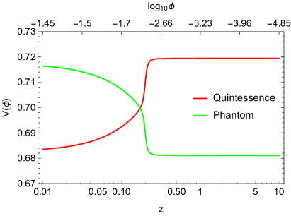
Such transitions in the dark energy equation of state are in principle well-motivated and can easily happen within the context of a minimally coupled scalar field in general relativity (GR), either of the quintessence or phantom type. For example, in Fig. 1 we show a transition in the dark energy equation of state (left panel) and how it can be caused by a sharp transition in a quintessence (red line) or phantom (green line) potential (right panel), with the scalar field running down/up the potential respectively. For this plot we assumed, as an example, a smooth transition and reconstructed the potentials following the procedure of Ref. Sahni and Starobinsky (2006), assuming , , for quintessence and phantom fields. By adjusting the aforementioned parameters, one may tune both the steepness and the redshift of the transition.
In order to constrain these transition models we use the following data combination:
- •
- •
-
•
The latest SnIa dataset (Pantheon) presented in Ref. Scolnic et al. (2018b).
- •
To analyze the data and obtain the best fit parameters we modify the publicly available CLASS code333For a step-by-step guide for the modifications implemented in CLASS, see this file. and perform the Monte Carlo Markov Chain (MCMC) analysis using the publicly available MontePython code Brinckmann and Lesgourgues (2019); Audren et al. (2013); Blas et al. (2011).
These models by construction provide a great amount of flexibility in fitting the observational data since they can mimic CDM for , while being fully consistent with local measurements of . In the case of the transition occurring at very low redshifts where there are almost no available data, i.e. at , we would normally anticipate a fit even better to that of CDM due to the extra parameter in the context of . However, then there would be no tension, since the local measurement of should coincide with the measurement of Planck if the transition is taken into account (a shift of implies a shift of since the two parameters are degenerate).
Interestingly there are some works that use data with , such as the extended Pantheon dataset of the latest SH0ES analysis (Panteon+) Riess et al. (2021b) as well as the analyses of Refs. Dhawan et al. (2020); Perivolaropoulos and Skara (2021b), that can be used to search self-consistently for a transition in at using the combined Cepheid and SnIa data. Regarding the Pantheon+ dataset however, not only the data are not publicly available yet but also in our analysis we are simultaneously marginalizing over and . We also stress that we are not including the full covariance between calibrators and supernovae as in the latest SH0ES analysis. Regarding Ref. Dhawan et al. (2020), the analysis makes no attempt to investigate an transition or to constrain variations of for since this redshift region is not in the Hubble flow and thus it can not be reliably constrained. In contrast, it demonstrates that variations of the parametrization in the Hubble flow (for ) do not affect the best fit value of . This result could have been anticipated by the fact that (almost) all parametrizations reduce to a cosmographic expansion in the range where the fit for is performed.
In addition, a separate analysis of Ref. Perivolaropoulos and Skara (2021b), focusing on the Cepheid+SnIa data for , has found hints for a transition in the Cepheid absolute magnitude and in the color luminosity parameter which, if taken into account, make the value of absolute magnitude of SnIa consistent with its inverse distance ladder value, thus resolving the Hubble tension.
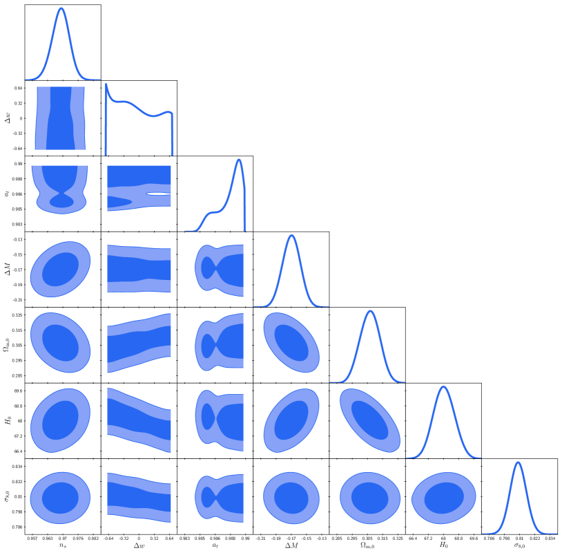
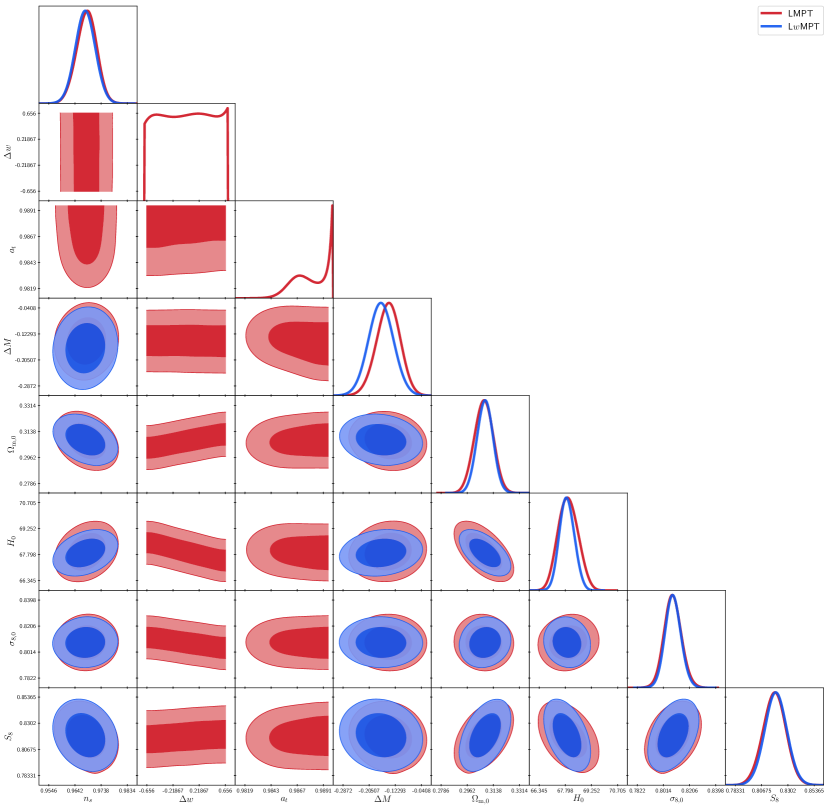
Hence, in what follows we impose a prior of that corresponds to , since any lower value of cannot be probed via the considered Hubble flow data. Moreover, we use a prior of . The best fit values of the model with are shown in Table 1, while the corresponding contours are shown in Fig. 2. In Table 1 we also include the parameter that arises for with corresponding to the Cepheid-calibrated value of the SnIa absolute magnitude.
| Parameter | best-fit | mean | 95.5% lower | 95.5% upper |
|---|---|---|---|---|
| unconstrained | unconstrained | unconstrained | unconstrained | |
| Parameter | best-fit | mean | 95.5% lower | 95.5% upper |
|---|---|---|---|---|
From Table 1, we see that the parameter (or equivalently ) approaches the highest (lowest) value imposed by the data in order to achieve the best possible quality of fit favoring a transition at very low redshifts. Moreover, the posterior probability of appears to be bimodal. The reason for this behavior may be seen e.g. in Fig. 9 of Ref. Alestas et al. (2021a) or in Fig. 3 of Ref. Camarena and Marra (2021) where the lowest bin for the SnIa absolute magnitude shows a rise that may be interpreted as a hint for a transition at (this is expressed by the first plato-peak for the likelihood of at ). The higher peak however occurs at indicating that the minimum for the transition redshift is at or below (no clear hint for a transition in the Hubble flow). However, given that the data do not extend to more recent times than , the best fit is at as it is explicitly written in Table 1 and the higher peak at can only be interpreted as a lower bound for the value if the transition occurs at more recent times. We thus chose to neglect this second peak.
The timing of the transition is not particularly fine-tuned due to the fact that at very low redshifts dark energy has started to dominate in the Universe. Since at that time , new physics could possibly emerge. Furthermore, in previous analyses by some of the authors of the current work Kazantzidis and Perivolaropoulos (2020); Kazantzidis et al. (2021) a tomographic analysis of the Pantheon dataset has been performed. In both of these references, it has been shown that for the redshift binned best fit CDM parameter values for the parameter (as well as ) vary around the full dataset fit value (assumed constant) by up to . This variation is significantly smaller than the variation required for the resolution of the Hubble tension (see e.g. the left panel of Fig. 1 of Kazantzidis et al. (2021)). Most importantly, however, we observe that despite allowing for an extra degree of freedom induced by having , this parameter seems to be ignored by the data.
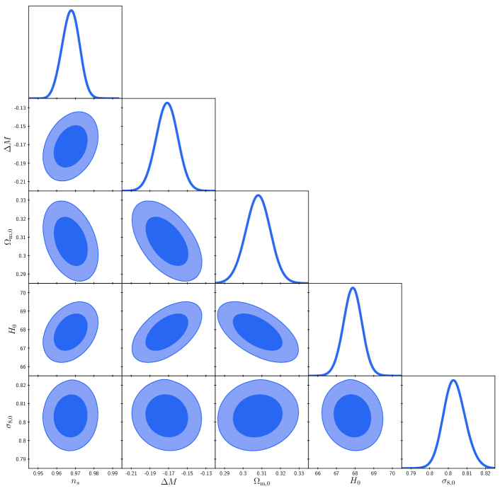
Since is favored by the data, the parameter becomes irrelevant due to the fact that for , would modify the expansion rate only in a region where there are no data available (). This carries the implication that a transition is perhaps not needed in order to obtain the best quality of fit to the data444The transition however may be required for theoretical reasons. In scalar tensor theories a gravitational transition to weaker gravity at early times may require a simultaneous transition to at late times.. We thus repeat the analysis considering only an transition (“Late Transition” - ), setting and (or equivalently ), which is basically the maximum of the posterior of for the model. We obtain the best fit and mean values as indicated in Table 2; the contours are shown in Fig. 3.
As we can see comparing Tables 1, 2 and Figs. 2, 3 the introduction of has practically no effect on the quality of fit, i.e. on the value. Moreover, the mismatch between the local calibration of the SnIa absolute magnitude and the value inferred from the other probes is very significant, suggesting that the designation tension/crisis is suitable to describe the crisis Camarena and Marra (2021); Efstathiou (2021). Finally, it is interesting to note that the inferred value of mag agrees well with the constraint mag that was obtained using the parametric-free inverse distance ladder of Ref. Camarena and Marra (2020b).
So, some natural questions that arise are the following: “How do the transition models and compare to some other popular dark energy models in the literature that also try to address the Hubble tension?” and “Can these models provide an value that is consistent with the Cepheid measurement as the transition models that we discussed?” These questions will be addressed in the following section, where we perform a comparison between some popular dark energy parametrizations (smooth deformation dark energy models) with the transition models and .
| Parameters | CDM | CDM | CPL | PEDE | ||
| - | - | - | - | |||
| - | - | - | - | |||
| - | - | - | unconstrained | - | - | |
| - | - | - | - | - | ||
| - | - | - | - | |||
| - | - | - | - | - | ||
| - |
III Comparison of Dark Energy Models
In order to truly resolve the tension, a dark energy model should not only provide a consistent measurement for , but also maintain a quality of fit comparable (or even better) to CDM with low- data (BAO and SnIa), as discussed earlier. In this section, we consider some popular dark energy models, that have been suggested as being capable of addressing the tension, following three different methods:
- 1.
-
2.
Analyze all models including the local Cepheid-calibrated prior by SH0ES (Camarena and Marra, 2021):
(3) - 3.
The deformation dark energy models that we consider in this work include the CDM model, i.e. a model with a constant equation of state , assuming a flat Universe and cold dark matter, that is described by a Hubble parameter of the form (neglecting radiation and neutrinos at late times)
| (4) |
which for reduces to the usual Hubble parameter for the CDM model. Moreover, we consider the Chevallier-Polarski-Linder (CPL) parametrization, with a dark energy equation of state Chevallier and Polarski (2001); Linder (2003)
| (5) |
where and are free parameters. The corresponding Hubble parameter for the CPL model is the following
| (6) |
Furthermore, we consider the phenomenologically emergent dark energy (PEDE) model which shows significant promise in resolving the problem. This model was introduced in Ref. Li and Shafieloo (2019) and has an equation of state of the form
| (7) |
with a corresponding Hubble parameter of the form
| (8) |
The main advantage of the aforementioned parametrization is that it has the same number of degrees of freedom as CDM. Finally, we consider the transition models with and with described in Sec. II, as well as the CDM model itself, thus having a total of six different models.
| Parameters | CDM | CDM | CPL | PEDE | ||
| - | - | - | - | |||
| - | - | - | - | |||
| - | - | - | unconstrained | - | - | |
| - | - | - | - | - | ||
| - | - | - | - | |||
| - | - | - | - | - | ||
| - |

| Gaussian Prior Case | |||
|---|---|---|---|
| CDM | |||
| CDM | |||
| CPL | |||
| PEDE |
III.1 Dark energy models comparison using a narrow flat prior on mag
We perform the MCMC analysis using the likelihoods described in Section II and imposing a narrow flat prior on the SnIa absolute magnitude mag, that is, forcing all models to be consistent with the Cepheid measurement . Rigorously, this prior is artificial as the correct prior is the Gaussian one of Eq. (3). However, the use of this narrow prior will be useful to understand the impact of the local calibration on the quality of fit of the various models.
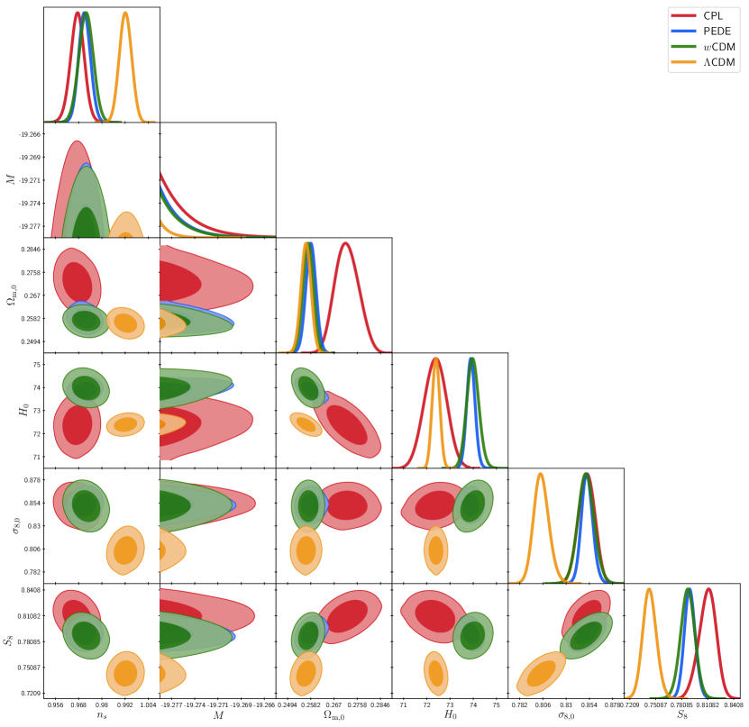
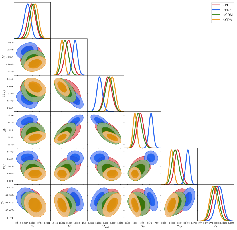
For the transition models and , we use Eq. (1) for the SnIa absolute magnitude and leave as a free variable. Thus, these are the only models that can, by construction, escape from the imposed prior. The constraints on the cosmological parameters as well as the – confidence contours of the corresponding parameters of the models are shown in Table 3 and Fig. 4 respectively. For the sake of clarity, contour plots for the and models are displayed separately. In this case, the analysis with a narrow flat prior on produces same constraints as those showed as Fig. 3 and Fig. 2 for the and models, respectively. A wider flat prior would lead (as in the case of a Gaussian prior of Table 4 that follows) the best fit value of for most models to be very close to the CMB inferred value of with an error bar which makes it inconsistent with the Cepheid inferred vale . In view of the degeneracy of with , this tension is closely related with the tension. A similar (but milder) tension occurs also in the case of a Gaussian prior on as indicated in Table 4.
All models, except the with and with , give an value that is consistent with the SH0ES determination of Riess et al. (2021a) and , i.e. the lowest eligible value of the prior that we imposed, displaying their tendency to provide a significantly lower value for . On the other hand, the transition models provide a value close (within the level) to the typical Planck18/CDM value, providing at the same time as expected.
Note that the CDM model has a very bad fit to the data as compared to CDM, CPL and PEDE. This is due to the fact that, having fixed to the local value, supernova data constrain the CDM model’s luminosity distance to values that are at odds with CMB and BAO. This clearly shows how the CDM model cannot possibly solve the crisis Camarena and Marra (2021); Efstathiou (2021). The more flexible CDM, CPL and PEDE models fare much better but still much worse than the and models which can fit all observables well.
All the models are forced to be consistent with the local Cepheid-calibrated value at the 1 level. As a result, in order to achieve consistency with the values of the other parameters differ significantly from the relevant CDM values. Also, the imposed significantly higher () than the best fit inverse distance ladder value () forces the MCMC process to restrict the rest of the parameters, thus explaining the extremely low uncertainties in order to achieve the best possible quality of fit to the data. We also stress that the peak structure of the CMB in the damping tail constrains very well the combination . Therefore, once we force - to be in agreement with SH0ES, we need a lower value of different from CDM to compensate for the higher value and keep the peak structure unaltered. Once we relax the prior (Table 4) can go back to the CDM value.
III.2 Dark energy models comparison using the local Cepheid prior on
Here, we adopt the local Gaussian prior of Eq. (3). The constraints on cosmological parameters are given in Table 4, while the corresponding – confidence contours are shown in Fig. 5. The transition / models fare significantly better than the other models, providing an absolute magnitude that is consistent with the Cepheid calibration of Eq. (3). The CDM and CPL models achieve a slightly better fit to data as compared to CDM, while the PEDE model has a significantly worse fit to data, in agreement with previous findings Pan et al. (2020b). Note that constraints for the and models have been not included in Fig. 5 for the sake of clarity. Constraints for these model are instead showed in Fig. 8 of the Appendix B.
III.3 Model selection
To select the best model one cannot just look at the quality of fit but it is essential to include the information on the number of parameters and their priors. Here, we only consider the case of Section III.2 as it uses the actual Cepheid prior of Eq. (3) from SH0ES. We adopt two approaches. First, we consider the Akaike Information Criterion (AIC) Akaike (1974); Nesseris and Garcia-Bellido (2013), defined as
| (9) |
where corresponds to the total number of free parameters of the considered model and corresponds to the maximum likelihood. This criterion penalizes a model for any extra parameters. Using Eq. (9) we calculate the AIC values for all the models of Table 4 and construct the corresponding differences , see Table 5. If , then the compared models can be interpreted as consistent with each other, while if it is an indication that the model with the larger AIC value is disfavored Nesseris and Garcia-Bellido (2013). We can see that the / models are strongly favored over CDM, and that the PEDE model is strongly disfavored.
We also use the MCEvidence package Heavens et al. (2017) in order to compute the Bayesian evidences (marginal likelihoods) of each model of Table 4 using their respective MCMC chains. This algorithm obtains the posterior for the marginal likelihood, using the -th nearest-neighbour Mahalanobis distances Mahalanobis (1936) in the parameter space. In our analysis we have adopted the case to minimize the effects of the inaccuracies associated with larger dimensions of the parameter space and smaller sample sizes. The strength of the evidence presented in favor or against a model in a comparison, can be found using the revised Jeffreys’ scale Trotta (2008). Specifically, in a comparison between two models via the Bayes factor (ratio of evidences), if the models are comparable with none of them being favored, for one model shows weak evidence in its favor, if the model in question has moderate evidence on its side, and lastly in the case of one model is strongly favored over the other. From Table 5 one can see that PEDE is strongly disfavored, CDM and CPL weakly favored and disfavored, respectively, and that the / models are strongly favored over CDM.
IV Discussion and conclusions
We have investigated the quality of fit to cosmological data of five models that attempt to solve the crisis. Besides the standard CDM model, we considered three smooth deformation models (CDM, CPL and PEDE) and two models that allow for a sudden transition of the SnIa absolute magnitude at a recent cosmological redshift . We performed model selection via the Akaike Information Criterion and the Bayes factor. This is a more detailed and extended fit to the data that includes the full CMB angular power spectrum, instead of just the peak locations, discussed in the previous studies Alestas et al. (2021a); Marra and Perivolaropoulos (2021) that introduced the ultra-late transition idea. We have also included additional cosmological models to compare the fit with the transition models and implemented different priors and model selection criteria.
We found that the transition models are strongly favored with respect to the CDM model. We also found that PEDE is strongly disfavored and that CDM and CPL are weakly favored and disfavored, respectively. Specifically, only -transition models are able to maintain consistency with the SnIa absolute magnitude measured by Cepheid calibrators while at the same time maintaining a quality of fit to the cosmological data at that is identical with that of CDM.
| Parameters | CDM | CDM | CPL | PEDE | ||
| - | - | - | - | |||
| - | - | - | - | |||
| - | - | - | - | - | ||
| - | - | - | - | - | ||
| - | - | - | - | |||
| - | - | - | - | - | ||
| - |
The required transition with magnitude can be induced by a corresponding transition of the effective gravitational constant which determines the strength of the gravitational interactions Marra and Perivolaropoulos (2021). The corresponding magnitude of the transition depends on the power value of the expression that connects the evolving Newton’s constant with the absolute luminosity of a SnIa:
| (10) |
In the case of the and transition models the transition in implies a transition in . In particular, for , it is:
| (11) |
while for we have . Since, , we can assume without loss of generality that , so it is straightforward to show that Eq. (10) corresponds to
| (12) |
Using the definition (11), for , we have
| (13) |
Therefore, substituting (13) in (12) and solving with respect to , we derive
| (14) |
We can constrain based on Eq. (14) and the fact that it obeys the general bounds (the corresponds to the CDM /GR case where ). Taking the absolute value of Eq. (14) and setting from Table 2 the 2- upper bound mag and Alvey et al. (2020), a measurement obtained using up to date primitive element abundances, cosmic microwave background as well as nuclear and weak reaction rates, assumes the following range
| (15) |
Similarly, if we consider the constraint from the Hubble diagram SnIa Gaztanaga et al. (2009), a measurement derived using luminous red galaxies, as well as from Paleontology Uzan (2003), a measurement obtained using the age of bacteria and algae, that indicate , we derive
| (16) |
This range includes the simple expectation that emerges if we assume that the SnIa absolute luminosity is proportional to the Chandrasekhar mass which leads to .
If the transition is due to a gravitational transition with a lower value of at then this class of models also has the potential to address the growth tension as discussed in previous studies Marra and Perivolaropoulos (2021). It should also be stressed that such a gravitational transition would be consistent with solar system tests of modified gravities without the need for screening since the value of is predicted to be constant at and therefore no modification of the planetary orbits is expected since the time these orbits have been monitored. However, at the time of the gravitational transition (about ago) a disruption of the planetary orbits and comets is expected Perivolaropoulos (2022). Such a prediction may be consistent with the observational fact that the rate of comets that hit the Earth and the Moon has increased by a factor of 2-3 during the past Shoemaker (1998); Gehrels (1995); McEwen et al. (1997); Grier et al. (2001); Ward and Day (2007).
As discussed in, e.g., Refs. Livio and Mazzali (2018); Jha et al. (2019); Flörs et al. (2020), SnIa progenitors are not necessarily Chandrasekhar-mass white dwarfs and a significant fraction can arise from sub-Chandrasekhar explosions. While this surely calls for a more detailed analysis of the dependence of the SnIa luminosity on , one must note that the Chandrasekhar mass scale is a fundamental reference scale that plays an important role in all SnIa explosions. However, a nontrivial relation between progenitors and SnIa could again imply that the relation of Eq. (10) could feature a value of different from corresponding to the simplest case where .
Therefore, interesting extensions of our analysis include the following:
-
•
The search for traces or constraints of a gravitational transition in geological, solar system and astrophysical data.
-
•
The construction of simple theoretical modified gravity models that can naturally induce the required transition of the effective Newton’s at low redshifts () perhaps avoiding fine tuning issues.
-
•
The possible identification of alternative non-gravitational physical mechanisms that could induce the transition of SnIa at low redshifts.
-
•
The search for systematic effects in the Cepheid data and parameters that could mimic such a transition and/or induce a higher value of for SnIa than the one currently accepted.
In conclusion the -transition class of models is an interesting new approach to the Hubble and possibly to the growth tension that deserves further investigation.
Numerical Analysis Files: The numerical files for the reproduction of the figures can be found in the GitHub repository H0_Model_Comparison under the MIT license.
Acknowledgements
The MCMC chains were produced in the Hydra cluster at the Instituto de Física Teórica (IFT) in Madrid and in the CHE cluster, managed and funded by COSMO/CBPF/MCTI, with financial support from FINEP and FAPERJ, and operating at the Javier Magnin Computing Center/CBPF, using MontePython/CLASS Brinckmann and Lesgourgues (2019); Audren et al. (2013); Blas et al. (2011). GA’s research was supported by the project “Dioni: Computing Infrastructure for Big-Data Processing and Analysis” (MIS No. 5047222) co-funded by European Union (ERDF) and Greece through Operational Program “Competitiveness, Entrepreneurship and Innovation”, NSRF 2014-2020. DC thanks CAPES for financial support. EDV is supported by a Royal Society Dorothy Hodgkin Research Fellowship. LK is co-financed by Greece and the European Union (European Social Fund- ESF) through the Operational Programme “Human Resources Development, Education and Lifelong Learning” in the context of the project “Strengthening Human Resources Research Potential via Doctorate Research – 2nd Cycle” (MIS-5000432), implemented by the State Scholarships Foundation (IKY). VM thanks CNPq (Brazil) and FAPES (Brazil) for partial financial support. This project has received funding from the European Union’s Horizon 2020 research and innovation programme under the Marie Skłodowska-Curie grant agreement No 888258. SN acknowledges support from the Research Project PGC2018-094773-B-C32, the Centro de Excelencia Severo Ochoa Program SEV-2016-0597 and the Ramón y Cajal program through Grant No. RYC-2014-15843.
Appendix A Analysis of the Dark Energy Models including the Local Measurement
We repeat the analysis for the models in question including the latest SH0ES measurement, Riess et al. (2021a), instead of the local prior on of Eq. (3) that was adopted in Section III.2. This is done in order to show that, despite the strong constraining nature of the SH0ES measurement, the obtained absolute magnitude for smooth deformation models are inconsistent with the measured Cepheid absolute magnitude of Eq. (3). It is worth stressing that it is preferable to adopt the local prior on for the following reasons (Camarena and Marra, 2021): i) one avoids double counting low- supernova, ii) the statistical information on is included in the analysis, iii) one avoids adopting a low- cosmography, with possibly wrong parameters, in the analysis.
Repeating the MCMC analysis and using the same likelihoods described in Section II, we obtain the constraints on cosmological parameters for all the models as shown in Table 6. The corresponding – confidence contours of the common parameters of the models are illustrated in Fig. 6. Constraints for the and models have been not included in Fig. 6, instead we show those constraints in Fig. 9.
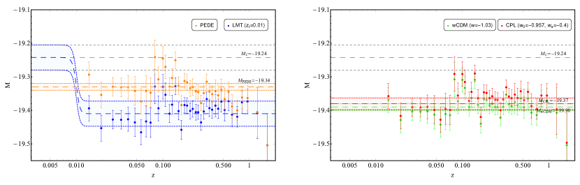
Clearly, all of the considered models (except the models with transitions) tend to prefer a significantly lower value for (which is considered to be constant) compared to . This is also evident in Fig. 7, where the best fit absolute magnitude of the binned Pantheon data is shown. In particular, in the case where no prior on is imposed, two of the considered models, i.e. CDM and CPL, produce a best fit value that is inconsistent with the SH0ES measurement Riess et al. (2021a) at more than . Regarding the with , even with the SH0ES measurement, the best fit value of parameter remains unaffected, continuing to favor a transition at very low redshifts. Conclusively, even though the majority of dark energy models discussed in this work (except PEDE and ) display a better quality of fit to the data than that of CDM (cyan row of Table 6), they fail to give an value consistent with the measurement (except the and models) despite the fact that some of them (such as PEDE) provide a measurement, that is consistent with the SH0ES measurement at the level.
Appendix B Contours plots for the and models
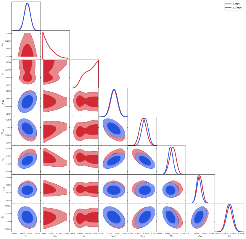
Here, we show contours plots relative to analyses with the models and . Fig. 8 shows the – confidence contours of cosmological parameters of models and for the analysis with the Gaussian prior on . On the other hand, Fig. 9 shows the – confidence contours of cosmological parameters of models and for the analysis that includes a Gaussian prior on .
References
- Di Valentino et al. (2021a) Eleonora Di Valentino et al., “Snowmass2021 - Letter of interest cosmology intertwined I: Perspectives for the next decade,” Astropart. Phys. 131, 102606 (2021a), arXiv:2008.11283 [astro-ph.CO] .
- Di Valentino et al. (2021b) Eleonora Di Valentino et al., “Snowmass2021 - Letter of interest cosmology intertwined II: The hubble constant tension,” Astropart. Phys. 131, 102605 (2021b), arXiv:2008.11284 [astro-ph.CO] .
- Di Valentino et al. (2021c) Eleonora Di Valentino et al., “Cosmology intertwined III: and ,” Astropart. Phys. 131, 102604 (2021c), arXiv:2008.11285 [astro-ph.CO] .
- Di Valentino et al. (2021d) Eleonora Di Valentino et al., “Snowmass2021 - Letter of interest cosmology intertwined IV: The age of the universe and its curvature,” Astropart. Phys. 131, 102607 (2021d), arXiv:2008.11286 [astro-ph.CO] .
- Perivolaropoulos and Skara (2021a) Leandros Perivolaropoulos and Foteini Skara, “Challenges for CDM: An update,” (2021a), arXiv:2105.05208 [astro-ph.CO] .
- Saridakis et al. (2021) Emmanuel N. Saridakis et al. (CANTATA), “Modified Gravity and Cosmology: An Update by the CANTATA Network,” (2021), arXiv:2105.12582 [gr-qc] .
- Verde et al. (2019) L. Verde, T. Treu, and A. G. Riess, “Tensions between the Early and the Late Universe,” Nature Astron. 3, 891 (2019), arXiv:1907.10625 [astro-ph.CO] .
- Riess (2019) Adam G. Riess, “The Expansion of the Universe is Faster than Expected,” Nature Rev. Phys. 2, 10–12 (2019), arXiv:2001.03624 [astro-ph.CO] .
- Di Valentino (2021) Eleonora Di Valentino, “A combined analysis of the late time direct measurements and the impact on the Dark Energy sector,” Mon. Not. Roy. Astron. Soc. 502, 2065–2073 (2021), arXiv:2011.00246 [astro-ph.CO] .
- Di Valentino et al. (2021e) Eleonora Di Valentino, Olga Mena, Supriya Pan, Luca Visinelli, Weiqiang Yang, Alessandro Melchiorri, David F. Mota, Adam G. Riess, and Joseph Silk, “In the Realm of the Hubble tension a Review of Solutions,” (2021e), 10.1088/1361-6382/ac086d, arXiv:2103.01183 [astro-ph.CO] .
- Shah et al. (2021) Paul Shah, Pablo Lemos, and Ofer Lahav, “A buyer’s guide to the Hubble Constant,” (2021), arXiv:2109.01161 [astro-ph.CO] .
- Aghanim et al. (2020a) N. Aghanim et al. (Planck), “Planck 2018 results. VI. Cosmological parameters,” Astron. Astrophys. 641, A6 (2020a), arXiv:1807.06209 [astro-ph.CO] .
- Riess et al. (2021a) Adam G. Riess, Stefano Casertano, Wenlong Yuan, J. Bradley Bowers, Lucas Macri, Joel C. Zinn, and Dan Scolnic, “Cosmic Distances Calibrated to 1% Precision with Gaia EDR3 Parallaxes and Hubble Space Telescope Photometry of 75 Milky Way Cepheids Confirm Tension with CDM,” Astrophys. J. Lett. 908, L6 (2021a), arXiv:2012.08534 [astro-ph.CO] .
- Aiola et al. (2020) Simone Aiola et al. (ACT), “The Atacama Cosmology Telescope: DR4 Maps and Cosmological Parameters,” JCAP 12, 047 (2020), arXiv:2007.07288 [astro-ph.CO] .
- Dutcher et al. (2021) D. Dutcher et al. (SPT-3G), “Measurements of the E-Mode Polarization and Temperature-E-Mode Correlation of the CMB from SPT-3G 2018 Data,” (2021), arXiv:2101.01684 [astro-ph.CO] .
- Alam et al. (2021) Shadab Alam et al. (eBOSS), “Completed SDSS-IV extended Baryon Oscillation Spectroscopic Survey: Cosmological implications from two decades of spectroscopic surveys at the Apache Point Observatory,” Phys. Rev. D 103, 083533 (2021), arXiv:2007.08991 [astro-ph.CO] .
- Soltis et al. (2021) John Soltis, Stefano Casertano, and Adam G. Riess, “The Parallax of Centauri Measured from Gaia EDR3 and a Direct, Geometric Calibration of the Tip of the Red Giant Branch and the Hubble Constant,” Astrophys. J. Lett. 908, L5 (2021), arXiv:2012.09196 [astro-ph.GA] .
- Pesce et al. (2020) D. W. Pesce et al., “The Megamaser Cosmology Project. XIII. Combined Hubble constant constraints,” Astrophys. J. Lett. 891, L1 (2020), arXiv:2001.09213 [astro-ph.CO] .
- Kourkchi et al. (2020) Ehsan Kourkchi, R. Brent Tully, Gagandeep S. Anand, Helene M. Courtois, Alexandra Dupuy, James D. Neill, Luca Rizzi, and Mark Seibert, “Cosmicflows-4: The Calibration of Optical and Infrared Tully–Fisher Relations,” Astrophys. J. 896, 3 (2020), arXiv:2004.14499 [astro-ph.GA] .
- Schombert et al. (2020) James Schombert, Stacy McGaugh, and Federico Lelli, “Using the Baryonic Tully–Fisher Relation to Measure H o,” Astron. J. 160, 71 (2020), arXiv:2006.08615 [astro-ph.CO] .
- Blakeslee et al. (2021) John P. Blakeslee, Joseph B. Jensen, Chung-Pei Ma, Peter A. Milne, and Jenny E. Greene, “The Hubble Constant from Infrared Surface Brightness Fluctuation Distances,” Astrophys. J. 911, 65 (2021), arXiv:2101.02221 [astro-ph.CO] .
- Freedman (2021) Wendy L. Freedman, “Measurements of the Hubble Constant: Tensions in Perspective,” (2021), arXiv:2106.15656 [astro-ph.CO] .
- Anand et al. (2021) Gagandeep S. Anand, R. Brent Tully, Luca Rizzi, Adam G. Riess, and Wenlong Yuan, “Comparing Tip of the Red Giant Branch Distance Scales: An Independent Reduction of the Carnegie-Chicago Hubble Program and the Value of the Hubble Constant,” (2021), arXiv:2108.00007 [astro-ph.CO] .
- Birrer et al. (2020) S. Birrer et al., “TDCOSMO - IV. Hierarchical time-delay cosmography – joint inference of the Hubble constant and galaxy density profiles,” Astron. Astrophys. 643, A165 (2020), arXiv:2007.02941 [astro-ph.CO] .
- Hildebrandt et al. (2017) H. Hildebrandt et al., “KiDS-450: Cosmological parameter constraints from tomographic weak gravitational lensing,” Mon. Not. Roy. Astron. Soc. 465, 1454 (2017), arXiv:1606.05338 [astro-ph.CO] .
- Nesseris et al. (2017) Savvas Nesseris, George Pantazis, and Leandros Perivolaropoulos, “Tension and constraints on modified gravity parametrizations of from growth rate and Planck data,” Phys. Rev. D 96, 023542 (2017), arXiv:1703.10538 [astro-ph.CO] .
- Macaulay et al. (2013) Edward Macaulay, Ingunn Kathrine Wehus, and Hans Kristian Eriksen, “Lower Growth Rate from Recent Redshift Space Distortion Measurements than Expected from Planck,” Phys. Rev. Lett. 111, 161301 (2013), arXiv:1303.6583 [astro-ph.CO] .
- Kazantzidis and Perivolaropoulos (2018) Lavrentios Kazantzidis and Leandros Perivolaropoulos, “Evolution of the tension with the Planck15/CDM determination and implications for modified gravity theories,” Phys. Rev. D 97, 103503 (2018), arXiv:1803.01337 [astro-ph.CO] .
- Skara and Perivolaropoulos (2020) F. Skara and L. Perivolaropoulos, “Tension of the statistic and redshift space distortion data with the Planck - model and implications for weakening gravity,” Phys. Rev. D 101, 063521 (2020), arXiv:1911.10609 [astro-ph.CO] .
- Kazantzidis and Perivolaropoulos (2019) Lavrentios Kazantzidis and Leandros Perivolaropoulos, “Is gravity getting weaker at low z? Observational evidence and theoretical implications,” preprint (arXiv:1907.03176) (2019), arXiv:1907.03176 [astro-ph.CO] .
- Perivolaropoulos and Kazantzidis (2019) Leandros Perivolaropoulos and Lavrentios Kazantzidis, “Hints of modified gravity in cosmos and in the lab?” Int. J. Mod. Phys. D 28, 1942001 (2019), arXiv:1904.09462 [gr-qc] .
- Karwal and Kamionkowski (2016) Tanvi Karwal and Marc Kamionkowski, “Dark energy at early times, the Hubble parameter, and the string axiverse,” Phys. Rev. D 94, 103523 (2016), arXiv:1608.01309 [astro-ph.CO] .
- Poulin et al. (2019) Vivian Poulin, Tristan L. Smith, Tanvi Karwal, and Marc Kamionkowski, “Early Dark Energy Can Resolve The Hubble Tension,” Phys. Rev. Lett. 122, 221301 (2019), arXiv:1811.04083 [astro-ph.CO] .
- Sakstein and Trodden (2020) Jeremy Sakstein and Mark Trodden, “Early Dark Energy from Massive Neutrinos as a Natural Resolution of the Hubble Tension,” Phys. Rev. Lett. 124, 161301 (2020), arXiv:1911.11760 [astro-ph.CO] .
- Niedermann and Sloth (2021) Florian Niedermann and Martin S. Sloth, “New early dark energy,” Phys. Rev. D 103, L041303 (2021), arXiv:1910.10739 [astro-ph.CO] .
- Hill et al. (2020) J. Colin Hill, Evan McDonough, Michael W. Toomey, and Stephon Alexander, “Early dark energy does not restore cosmological concordance,” Phys. Rev. D 102, 043507 (2020), arXiv:2003.07355 [astro-ph.CO] .
- Murgia et al. (2021) Riccardo Murgia, Guillermo F. Abellán, and Vivian Poulin, “Early dark energy resolution to the Hubble tension in light of weak lensing surveys and lensing anomalies,” Phys. Rev. D 103, 063502 (2021), arXiv:2009.10733 [astro-ph.CO] .
- D’Amico et al. (2021) Guido D’Amico, Leonardo Senatore, Pierre Zhang, and Henry Zheng, “The Hubble Tension in Light of the Full-Shape Analysis of Large-Scale Structure Data,” JCAP 05, 072 (2021), arXiv:2006.12420 [astro-ph.CO] .
- Gogoi et al. (2021) Antareep Gogoi, Ravi Kumar Sharma, Prolay Chanda, and Subinoy Das, “Early Mass-varying Neutrino Dark Energy: Nugget Formation and Hubble Anomaly,” Astrophys. J. 915, 132 (2021), arXiv:2005.11889 [astro-ph.CO] .
- Chudaykin et al. (2021) Anton Chudaykin, Dmitry Gorbunov, and Nikita Nedelko, “Exploring an early dark energy solution to the Hubble tension with Planck and SPTPol data,” Phys. Rev. D 103, 043529 (2021), arXiv:2011.04682 [astro-ph.CO] .
- Chudaykin et al. (2020) Anton Chudaykin, Dmitry Gorbunov, and Nikita Nedelko, “Combined analysis of Planck and SPTPol data favors the early dark energy models,” JCAP 08, 013 (2020), arXiv:2004.13046 [astro-ph.CO] .
- Agrawal et al. (2019) Prateek Agrawal, Francis-Yan Cyr-Racine, David Pinner, and Lisa Randall, “Rock ’n’ Roll Solutions to the Hubble Tension,” (2019), arXiv:1904.01016 [astro-ph.CO] .
- Niedermann and Sloth (2020) Florian Niedermann and Martin S. Sloth, “Resolving the Hubble Tension with New Early Dark Energy,” Phys. Rev. D 102, 063527 (2020), arXiv:2006.06686 [astro-ph.CO] .
- Ye and Piao (2020) Gen Ye and Yun-Song Piao, “Is the Hubble tension a hint of AdS phase around recombination?” Phys. Rev. D 101, 083507 (2020), arXiv:2001.02451 [astro-ph.CO] .
- Lin et al. (2019) Meng-Xiang Lin, Giampaolo Benevento, Wayne Hu, and Marco Raveri, “Acoustic Dark Energy: Potential Conversion of the Hubble Tension,” Phys. Rev. D 100, 063542 (2019), arXiv:1905.12618 [astro-ph.CO] .
- Braglia et al. (2020) Matteo Braglia, William T. Emond, Fabio Finelli, A. Emir Gumrukcuoglu, and Kazuya Koyama, “Unified framework for Early Dark Energy from -attractors,” (2020), arXiv:2005.14053 [astro-ph.CO] .
- Hill et al. (2021) J. Colin Hill et al., “The Atacama Cosmology Telescope: Constraints on Pre-Recombination Early Dark Energy,” (2021), arXiv:2109.04451 [astro-ph.CO] .
- Chang (2021) Chia-Feng Chang, “Imprint of Early Dark Energy in Stochastic Gravitational Wave Background,” (2021), arXiv:2107.14258 [astro-ph.CO] .
- Ye et al. (2021) Gen Ye, Jun Zhang, and Yun-Song Piao, “Resolving both and tensions with AdS early dark energy and ultralight axion,” (2021), arXiv:2107.13391 [astro-ph.CO] .
- Gómez-Valent et al. (2021) Adrià Gómez-Valent, Ziyang Zheng, Luca Amendola, Valeria Pettorino, and Christof Wetterich, “Early dark energy in the pre- and post-recombination epochs,” (2021), arXiv:2107.11065 [astro-ph.CO] .
- Jiang and Piao (2021) Jun-Qian Jiang and Yun-Song Piao, “Testing AdS early dark energy with Planck, SPTpol and LSS data,” (2021), arXiv:2107.07128 [astro-ph.CO] .
- Karwal et al. (2021) Tanvi Karwal, Marco Raveri, Bhuvnesh Jain, Justin Khoury, and Mark Trodden, “Chameleon Early Dark Energy and the Hubble Tension,” (2021), arXiv:2106.13290 [astro-ph.CO] .
- Poulin et al. (2021) Vivian Poulin, Tristan L. Smith, and Alexa Bartlett, “Dark Energy at early times and ACT: a larger Hubble constant without late-time priors,” (2021), arXiv:2109.06229 [astro-ph.CO] .
- Vagnozzi (2020) Sunny Vagnozzi, “New physics in light of the tension: An alternative view,” Phys. Rev. D 102, 023518 (2020), arXiv:1907.07569 [astro-ph.CO] .
- Seto and Toda (2021) Osamu Seto and Yo Toda, “Comparing early dark energy and extra radiation solutions to the Hubble tension with BBN,” Phys. Rev. D 103, 123501 (2021), arXiv:2101.03740 [astro-ph.CO] .
- Carneiro et al. (2019) S. Carneiro, P. C. de Holanda, C. Pigozzo, and F. Sobreira, “Is the tension suggesting a fourth neutrino generation?” Phys. Rev. D 100, 023505 (2019), arXiv:1812.06064 [astro-ph.CO] .
- Gelmini et al. (2021) Graciela B. Gelmini, Alexander Kusenko, and Volodymyr Takhistov, “Possible Hints of Sterile Neutrinos in Recent Measurements of the Hubble Parameter,” JCAP 06, 002 (2021), arXiv:1906.10136 [astro-ph.CO] .
- Gelmini et al. (2020) Graciela B. Gelmini, Masahiro Kawasaki, Alexander Kusenko, Kai Murai, and Volodymyr Takhistov, “Big Bang Nucleosynthesis constraints on sterile neutrino and lepton asymmetry of the Universe,” JCAP 09, 051 (2020), arXiv:2005.06721 [hep-ph] .
- D’Eramo et al. (2018) Francesco D’Eramo, Ricardo Z. Ferreira, Alessio Notari, and José Luis Bernal, “Hot Axions and the tension,” JCAP 11, 014 (2018), arXiv:1808.07430 [hep-ph] .
- Pandey et al. (2020) Kanhaiya L. Pandey, Tanvi Karwal, and Subinoy Das, “Alleviating the and anomalies with a decaying dark matter model,” JCAP 07, 026 (2020), arXiv:1902.10636 [astro-ph.CO] .
- Xiao et al. (2020) Linfeng Xiao, Le Zhang, Rui An, Chang Feng, and Bin Wang, “Fractional Dark Matter decay: cosmological imprints and observational constraints,” JCAP 01, 045 (2020), arXiv:1908.02668 [astro-ph.CO] .
- Nygaard et al. (2021) Andreas Nygaard, Thomas Tram, and Steen Hannestad, “Updated constraints on decaying cold dark matter,” JCAP 05, 017 (2021), arXiv:2011.01632 [astro-ph.CO] .
- Blinov et al. (2020) Nikita Blinov, Celeste Keith, and Dan Hooper, “Warm Decaying Dark Matter and the Hubble Tension,” JCAP 06, 005 (2020), arXiv:2004.06114 [astro-ph.CO] .
- Binder et al. (2018) Tobias Binder, Michael Gustafsson, Ayuki Kamada, Stefan Marinus Rodrigues Sandner, and Max Wiesner, “Reannihilation of self-interacting dark matter,” Phys. Rev. D 97, 123004 (2018), arXiv:1712.01246 [astro-ph.CO] .
- Choi et al. (2020) Gongjun Choi, Motoo Suzuki, and Tsutomu T. Yanagida, “Quintessence axion dark energy and a solution to the hubble tension,” Phys. Lett. B 805, 135408 (2020), arXiv:1910.00459 [hep-ph] .
- Di Valentino et al. (2018) Eleonora Di Valentino, Céline Bøehm, Eric Hivon, and François R. Bouchet, “Reducing the and tensions with Dark Matter-neutrino interactions,” Phys. Rev. D 97, 043513 (2018), arXiv:1710.02559 [astro-ph.CO] .
- Escudero and Witte (2020) Miguel Escudero and Samuel J. Witte, “A CMB search for the neutrino mass mechanism and its relation to the Hubble tension,” Eur. Phys. J. C 80, 294 (2020), arXiv:1909.04044 [astro-ph.CO] .
- Arias-Aragon et al. (2021) Fernando Arias-Aragon, Enrique Fernandez-Martinez, Manuel Gonzalez-Lopez, and Luca Merlo, “Neutrino Masses and Hubble Tension via a Majoron in MFV,” Eur. Phys. J. C 81, 28 (2021), arXiv:2009.01848 [hep-ph] .
- Blinov and Marques-Tavares (2020) Nikita Blinov and Gustavo Marques-Tavares, “Interacting radiation after Planck and its implications for the Hubble Tension,” JCAP 09, 029 (2020), arXiv:2003.08387 [astro-ph.CO] .
- Flambaum and Samsonov (2019) V. V. Flambaum and I. B. Samsonov, “Ultralight dark photon as a model for early universe dark matter,” Phys. Rev. D 100, 063541 (2019), arXiv:1908.09432 [astro-ph.CO] .
- Anchordoqui et al. (2021) Luis A. Anchordoqui, Eleonora Di Valentino, Supriya Pan, and Weiqiang Yang, “Dissecting the H0 and S8 tensions with Planck + BAO + supernova type Ia in multi-parameter cosmologies,” JHEAp 32, 121 (2021), arXiv:2107.13932 [astro-ph.CO] .
- Das (2021) Anirban Das, “Self-interacting neutrinos as a solution to the hubble tension?” in EPS Conference on High Energy Physics 2021 (2021) arXiv:2109.03263 [hep-ph] .
- Fernandez-Martinez et al. (2021) Enrique Fernandez-Martinez, Mathias Pierre, E. Pinsard, and Salvador Rosauro-Alcaraz, “Inverse Seesaw, dark matter and the Hubble tension,” (2021), arXiv:2106.05298 [hep-ph] .
- Feng et al. (2021) Lu Feng, Rui-Yun Guo, Jing-Fei Zhang, and Xin Zhang, “Cosmological search for sterile neutrinos after Planck 2018,” (2021), arXiv:2109.06111 [astro-ph.CO] .
- Ghosh et al. (2021) Subhajit Ghosh, Soubhik Kumar, and Yuhsin Tsai, “Free-streaming and Coupled Dark Radiation Isocurvature Perturbations: Constraints and Application to the Hubble Tension,” (2021), arXiv:2107.09076 [astro-ph.CO] .
- Hazra et al. (2019) Dhiraj Kumar Hazra, Arman Shafieloo, and Tarun Souradeep, “Parameter discordance in Planck CMB and low-redshift measurements: projection in the primordial power spectrum,” JCAP 04, 036 (2019), arXiv:1810.08101 [astro-ph.CO] .
- Keeley et al. (2020) Ryan E. Keeley, Arman Shafieloo, Dhiraj Kumar Hazra, and Tarun Souradeep, “Inflation Wars: A New Hope,” JCAP 09, 055 (2020), arXiv:2006.12710 [astro-ph.CO] .
- Nesseris et al. (2020) Savvas Nesseris, Domenico Sapone, and Spyros Sypsas, “Evaporating primordial black holes as varying dark energy,” Phys. Dark Univ. 27, 100413 (2020), arXiv:1907.05608 [astro-ph.CO] .
- Arendse et al. (2020) Nikki Arendse et al., “Cosmic dissonance: are new physics or systematics behind a short sound horizon?” Astron. Astrophys. 639, A57 (2020), arXiv:1909.07986 [astro-ph.CO] .
- Lin et al. (2021) Weikang Lin, Xingang Chen, and Katherine J. Mack, “Early-Universe-Physics Insensitive and Uncalibrated Cosmic Standards: Constraints on and Implications for the Hubble Tension,” (2021), arXiv:2102.05701 [astro-ph.CO] .
- Schöneberg et al. (2021) Nils Schöneberg, Guillermo Franco Abellán, Andrea Pérez Sánchez, Samuel J. Witte, Vivian Poulin, and Julien Lesgourgues, “The Olympics: A fair ranking of proposed models,” (2021), arXiv:2107.10291 [astro-ph.CO] .
- Jedamzik et al. (2020) Karsten Jedamzik, Levon Pogosian, and Gong-Bo Zhao, “Why reducing the cosmic sound horizon can not fully resolve the Hubble tension,” preprint (arXiv:2010.04158) (2020), arXiv:2010.04158 [astro-ph.CO] .
- Smith et al. (2020) Tristan L. Smith, Vivian Poulin, José Luis Bernal, Kimberly K. Boddy, Marc Kamionkowski, and Riccardo Murgia, “Early dark energy is not excluded by current large-scale structure data,” preprint (arXiv:2009.10740) (2020), arXiv:2009.10740 [astro-ph.CO] .
- Alestas et al. (2021a) George Alestas, Lavrentios Kazantzidis, and Leandros Perivolaropoulos, “ phantom transition at 0.1 as a resolution of the Hubble tension,” Phys. Rev. D 103, 083517 (2021a), arXiv:2012.13932 [astro-ph.CO] .
- Hryczuk and Jodłowski (2020) Andrzej Hryczuk and Krzysztof Jodłowski, “Self-interacting dark matter from late decays and the tension,” Phys. Rev. D 102, 043024 (2020), arXiv:2006.16139 [hep-ph] .
- Vattis et al. (2019) Kyriakos Vattis, Savvas M. Koushiappas, and Abraham Loeb, “Dark matter decaying in the late Universe can relieve the H0 tension,” Phys. Rev. D 99, 121302 (2019), arXiv:1903.06220 [astro-ph.CO] .
- Haridasu and Viel (2020) Balakrishna S. Haridasu and Matteo Viel, “Late-time decaying dark matter: constraints and implications for the -tension,” Mon. Not. Roy. Astron. Soc. 497, 1757–1764 (2020), arXiv:2004.07709 [astro-ph.CO] .
- Clark et al. (2021) Steven J. Clark, Kyriakos Vattis, and Savvas M. Koushiappas, “Cosmological constraints on late-Universe decaying dark matter as a solution to the tension,” Phys. Rev. D 103, 043014 (2021), arXiv:2006.03678 [astro-ph.CO] .
- Mawas et al. (2021) Ennis Mawas, Lauren Street, Richard Gass, and L. C. R. Wijewardhana, “Interacting dark energy axions in light of the Hubble tension,” (2021), arXiv:2108.13317 [astro-ph.CO] .
- Liu et al. (2021) Wenzhong Liu, Luis A. Anchordoqui, Eleonora Di Valentino, Supriya Pan, Yabo Wu, and Weiqiang Yang, “Constraints from High-Precision Measurements of the Cosmic Microwave Background: The Case of Disintegrating Dark Matter with or Dynamical Dark Energy,” (2021), arXiv:2108.04188 [astro-ph.CO] .
- Di Valentino et al. (2020a) Eleonora Di Valentino, Alessandro Melchiorri, Olga Mena, and Sunny Vagnozzi, “Interacting dark energy in the early 2020s: A promising solution to the and cosmic shear tensions,” Phys. Dark Univ. 30, 100666 (2020a), arXiv:1908.04281 [astro-ph.CO] .
- Di Valentino et al. (2020b) Eleonora Di Valentino, Alessandro Melchiorri, Olga Mena, and Sunny Vagnozzi, “Nonminimal dark sector physics and cosmological tensions,” Phys. Rev. D 101, 063502 (2020b), arXiv:1910.09853 [astro-ph.CO] .
- Yang et al. (2020a) Weiqiang Yang, Eleonora Di Valentino, Olga Mena, Supriya Pan, and Rafael C. Nunes, “All-inclusive interacting dark sector cosmologies,” Phys. Rev. D 101, 083509 (2020a), arXiv:2001.10852 [astro-ph.CO] .
- Di Valentino et al. (2021f) Eleonora Di Valentino, Alessandro Melchiorri, Olga Mena, Supriya Pan, and Weiqiang Yang, “Interacting Dark Energy in a closed universe,” Mon. Not. Roy. Astron. Soc. 502, L23–L28 (2021f), arXiv:2011.00283 [astro-ph.CO] .
- Yang et al. (2021a) Weiqiang Yang, Supriya Pan, Eleonora Di Valentino, Olga Mena, and Alessandro Melchiorri, “2021- Odyssey: Closed, Phantom and Interacting Dark Energy Cosmologies,” (2021a), arXiv:2101.03129 [astro-ph.CO] .
- Kumar and Nunes (2017) Suresh Kumar and Rafael C. Nunes, “Echo of interactions in the dark sector,” Phys. Rev. D 96, 103511 (2017), arXiv:1702.02143 [astro-ph.CO] .
- Kumar et al. (2019) Suresh Kumar, Rafael C. Nunes, and Santosh Kumar Yadav, “Dark sector interaction: a remedy of the tensions between CMB and LSS data,” Eur. Phys. J. C 79, 576 (2019), arXiv:1903.04865 [astro-ph.CO] .
- Lucca and Hooper (2020) Matteo Lucca and Deanna C. Hooper, “Shedding light on dark matter-dark energy interactions,” Phys. Rev. D 102, 123502 (2020), arXiv:2002.06127 [astro-ph.CO] .
- Yang et al. (2020b) Weiqiang Yang, Supriya Pan, Rafael C. Nunes, and David F. Mota, “Dark calling Dark: Interaction in the dark sector in presence of neutrino properties after Planck CMB final release,” JCAP 04, 008 (2020b), arXiv:1910.08821 [astro-ph.CO] .
- Martinelli et al. (2019) Matteo Martinelli, Natalie B. Hogg, Simone Peirone, Marco Bruni, and David Wands, “Constraints on the interacting vacuum–geodesic CDM scenario,” Mon. Not. Roy. Astron. Soc. 488, 3423–3438 (2019), arXiv:1902.10694 [astro-ph.CO] .
- Gómez-Valent et al. (2020) Adrià Gómez-Valent, Valeria Pettorino, and Luca Amendola, “Update on coupled dark energy and the tension,” Phys. Rev. D 101, 123513 (2020), arXiv:2004.00610 [astro-ph.CO] .
- Di Valentino et al. (2017) Eleonora Di Valentino, Alessandro Melchiorri, and Olga Mena, “Can interacting dark energy solve the tension?” Phys. Rev. D 96, 043503 (2017), arXiv:1704.08342 [astro-ph.CO] .
- Kumar and Nunes (2016) Suresh Kumar and Rafael C. Nunes, “Probing the interaction between dark matter and dark energy in the presence of massive neutrinos,” Phys. Rev. D 94, 123511 (2016), arXiv:1608.02454 [astro-ph.CO] .
- Yang et al. (2018) Weiqiang Yang, Supriya Pan, Eleonora Di Valentino, Rafael C. Nunes, Sunny Vagnozzi, and David F. Mota, “Tale of stable interacting dark energy, observational signatures, and the tension,” JCAP 09, 019 (2018), arXiv:1805.08252 [astro-ph.CO] .
- Pan et al. (2020a) Supriya Pan, Weiqiang Yang, and Andronikos Paliathanasis, “Non-linear interacting cosmological models after Planck 2018 legacy release and the tension,” Mon. Not. Roy. Astron. Soc. 493, 3114–3131 (2020a), arXiv:2002.03408 [astro-ph.CO] .
- Yao and Meng (2020) Yan-Hong Yao and Xin-He Meng, “A new coupled three-form dark energy model and implications for the tension,” Phys. Dark Univ. 30, 100729 (2020).
- Yao and Meng (2021) Yanhong Yao and Xin-He Meng, “Relieve the H0 tension with a new coupled generalized three-form dark energy model,” Phys. Dark Univ. 33, 100852 (2021), arXiv:2011.09160 [astro-ph.CO] .
- Pan et al. (2019a) Supriya Pan, Weiqiang Yang, Eleonora Di Valentino, Emmanuel N. Saridakis, and Subenoy Chakraborty, “Interacting scenarios with dynamical dark energy: Observational constraints and alleviation of the tension,” Phys. Rev. D 100, 103520 (2019a), arXiv:1907.07540 [astro-ph.CO] .
- Yang et al. (2019a) Weiqiang Yang, Olga Mena, Supriya Pan, and Eleonora Di Valentino, “Dark sectors with dynamical coupling,” Phys. Rev. D 100, 083509 (2019a), arXiv:1906.11697 [astro-ph.CO] .
- Pan et al. (2019b) Supriya Pan, Weiqiang Yang, Chiranjeeb Singha, and Emmanuel N. Saridakis, “Observational constraints on sign-changeable interaction models and alleviation of the tension,” Phys. Rev. D 100, 083539 (2019b), arXiv:1903.10969 [astro-ph.CO] .
- Amirhashchi and Yadav (2020) Hassan Amirhashchi and Anil Kumar Yadav, “Interacting Dark Sectors in Anisotropic Universe: Observational Constraints and Tension,” (2020), arXiv:2001.03775 [astro-ph.CO] .
- Gao et al. (2021) Li-Yang Gao, Ze-Wei Zhao, She-Sheng Xue, and Xin Zhang, “Relieving the H 0 tension with a new interacting dark energy model,” JCAP 07, 005 (2021), arXiv:2101.10714 [astro-ph.CO] .
- Lucca (2021) Matteo Lucca, “Multi-interacting dark energy and its cosmological implications,” (2021), arXiv:2106.15196 [astro-ph.CO] .
- Bertacca et al. (2011) Daniele Bertacca, Marco Bruni, Oliver F. Piattella, and Davide Pietrobon, “Unified Dark Matter scalar field models with fast transition,” JCAP 02, 018 (2011), arXiv:1011.6669 [astro-ph.CO] .
- Haridasu et al. (2021) Balakrishna S. Haridasu, Matteo Viel, and Nicola Vittorio, “Sources of -tension in dark energy scenarios,” Phys. Rev. D 103, 063539 (2021), arXiv:2012.10324 [astro-ph.CO] .
- Menci et al. (2020) N. Menci et al., “Constraints on Dynamical Dark Energy Models from the Abundance of Massive Galaxies at High Redshifts,” Astrophys. J. 900, 108 (2020), arXiv:2007.12453 [astro-ph.CO] .
- Yang et al. (2019b) Weiqiang Yang, Supriya Pan, Eleonora Di Valentino, Emmanuel N. Saridakis, and Subenoy Chakraborty, “Observational constraints on one-parameter dynamical dark-energy parametrizations and the tension,” Phys. Rev. D 99, 043543 (2019b), arXiv:1810.05141 [astro-ph.CO] .
- Di Valentino et al. (2020c) Eleonora Di Valentino, Alessandro Melchiorri, and Joseph Silk, “Cosmological constraints in extended parameter space from the Planck 2018 Legacy release,” JCAP 01, 013 (2020c), arXiv:1908.01391 [astro-ph.CO] .
- Di Valentino et al. (2020d) Eleonora Di Valentino, Ankan Mukherjee, and Anjan A. Sen, “Dark Energy with Phantom Crossing and the tension,” preprint (arXiv:2005.12587) (2020d), arXiv:2005.12587 [astro-ph.CO] .
- Di Valentino et al. (2020e) Eleonora Di Valentino, Eric V. Linder, and Alessandro Melchiorri, “ ex machina: Vacuum metamorphosis and beyond ,” Phys. Dark Univ. 30, 100733 (2020e), arXiv:2006.16291 [astro-ph.CO] .
- Yang et al. (2021b) Weiqiang Yang, Eleonora Di Valentino, Supriya Pan, and Olga Mena, “Emergent Dark Energy, neutrinos and cosmological tensions,” Phys. Dark Univ. 31, 100762 (2021b), arXiv:2007.02927 [astro-ph.CO] .
- Benaoum et al. (2020) H. B. Benaoum, Weiqiang Yang, Supriya Pan, and Eleonora Di Valentino, “Modified Emergent Dark Energy and its Astronomical Constraints,” (2020), arXiv:2008.09098 [gr-qc] .
- Yang et al. (2021c) Weiqiang Yang, Eleonora Di Valentino, Supriya Pan, Yabo Wu, and Jianbo Lu, “Dynamical dark energy after Planck CMB final release and tension,” Mon. Not. Roy. Astron. Soc. 501, 5845–5858 (2021c), arXiv:2101.02168 [astro-ph.CO] .
- Di Valentino et al. (2021g) Eleonora Di Valentino, Supriya Pan, Weiqiang Yang, and Luis A. Anchordoqui, “Touch of neutrinos on the vacuum metamorphosis: Is the solution back?” Phys. Rev. D 103, 123527 (2021g), arXiv:2102.05641 [astro-ph.CO] .
- Yang et al. (2021d) Weiqiang Yang, Eleonora Di Valentino, Supriya Pan, Arman Shafieloo, and Xiaolei Li, “Generalized emergent dark energy model and the Hubble constant tension,” Phys. Rev. D 104, 063521 (2021d), arXiv:2103.03815 [astro-ph.CO] .
- Li and Shafieloo (2019) Xiaolei Li and Arman Shafieloo, “A Simple Phenomenological Emergent Dark Energy Model can Resolve the Hubble Tension,” Astrophys. J. Lett. 883, L3 (2019), arXiv:1906.08275 [astro-ph.CO] .
- Pan et al. (2020b) Supriya Pan, Weiqiang Yang, Eleonora Di Valentino, Arman Shafieloo, and Subenoy Chakraborty, “Reconciling tension in a six parameter space?” JCAP 06, 062 (2020b), arXiv:1907.12551 [astro-ph.CO] .
- Rezaei et al. (2020) M. Rezaei, T. Naderi, M. Malekjani, and A. Mehrabi, “A Bayesian comparison between CDM and phenomenologically emergent dark energy models,” Eur. Phys. J. C 80, 374 (2020), arXiv:2004.08168 [astro-ph.CO] .
- Li and Shafieloo (2020) Xiaolei Li and Arman Shafieloo, “Evidence for Emergent Dark Energy,” (2020), arXiv:2001.05103 [astro-ph.CO] .
- Hernández-Almada et al. (2020) A. Hernández-Almada, Genly Leon, Juan Magaña, Miguel A. García-Aspeitia, and V. Motta, “Generalized Emergent Dark Energy: observational Hubble data constraints and stability analysis,” Mon. Not. Roy. Astron. Soc. 497, 1590–1602 (2020), arXiv:2002.12881 [astro-ph.CO] .
- Banihashemi et al. (2020) Abdolali Banihashemi, Nima Khosravi, and Amir H. Shirazi, “Phase transition in the dark sector as a proposal to lessen cosmological tensions,” Phys. Rev. D 101, 123521 (2020), arXiv:1808.02472 [astro-ph.CO] .
- Li et al. (2019) Xiaolei Li, Arman Shafieloo, Varun Sahni, and Alexei A. Starobinsky, “Revisiting Metastable Dark Energy and Tensions in the Estimation of Cosmological Parameters,” Astrophys. J. 887, 153 (2019), arXiv:1904.03790 [astro-ph.CO] .
- Yang et al. (2020c) Weiqiang Yang, Eleonora Di Valentino, Supriya Pan, Spyros Basilakos, and Andronikos Paliathanasis, “Metastable dark energy models in light of 2018 data: Alleviating the tension,” Phys. Rev. D 102, 063503 (2020c), arXiv:2001.04307 [astro-ph.CO] .
- Banihashemi et al. (2021) Abdolali Banihashemi, Nima Khosravi, and Arman Shafieloo, “Dark energy as a critical phenomenon: a hint from Hubble tension,” JCAP 06, 003 (2021), arXiv:2012.01407 [astro-ph.CO] .
- Solà et al. (2017) Joan Solà, Adrià Gómez-Valent, and Javier de Cruz Pérez, “The tension in light of vacuum dynamics in the Universe,” Phys. Lett. B 774, 317–324 (2017), arXiv:1705.06723 [astro-ph.CO] .
- Keeley et al. (2019) Ryan E. Keeley, Shahab Joudaki, Manoj Kaplinghat, and David Kirkby, “Implications of a transition in the dark energy equation of state for the and tensions,” JCAP 12, 035 (2019), arXiv:1905.10198 [astro-ph.CO] .
- Dutta et al. (2020) Koushik Dutta, Ruchika, Anirban Roy, Anjan A. Sen, and M. M. Sheikh-Jabbari, “Beyond CDM with low and high redshift data: implications for dark energy,” Gen. Rel. Grav. 52, 15 (2020), arXiv:1808.06623 [astro-ph.CO] .
- da Silva and Silva (2021a) W. J. C. da Silva and R. Silva, “Growth of matter perturbations in the extended viscous dark energy models,” Eur. Phys. J. C 81, 403 (2021a), arXiv:2011.09516 [astro-ph.CO] .
- Guo et al. (2019) Rui-Yun Guo, Jing-Fei Zhang, and Xin Zhang, “Can the tension be resolved in extensions to CDM cosmology?” JCAP 02, 054 (2019), arXiv:1809.02340 [astro-ph.CO] .
- da Silva and Silva (2021b) W. J. C. da Silva and R. Silva, “Cosmological Perturbations in the Tsallis Holographic Dark Energy Scenarios,” Eur. Phys. J. Plus 136, 543 (2021b), arXiv:2011.09520 [astro-ph.CO] .
- Di Valentino et al. (2019) Eleonora Di Valentino, Ricardo Z. Ferreira, Luca Visinelli, and Ulf Danielsson, “Late time transitions in the quintessence field and the tension,” Phys. Dark Univ. 26, 100385 (2019), arXiv:1906.11255 [astro-ph.CO] .
- Adler (2019) Stephen L. Adler, “Implications of a frame dependent dark energy for the spacetime metric, cosmography, and effective Hubble constant,” Phys. Rev. D 100, 123503 (2019), arXiv:1905.08228 [astro-ph.CO] .
- Akarsu et al. (2021) Özgür Akarsu, Suresh Kumar, Emre Özülker, and J. Alberto Vazquez, “CDM model: CDM model with a sign switching cosmological ‘constant’,” (2021), arXiv:2108.09239 [astro-ph.CO] .
- Benisty and Staicova (2021) David Benisty and Denitsa Staicova, “A preference for Dynamical Dark Energy?” (2021), arXiv:2107.14129 [astro-ph.CO] .
- Mazumdar et al. (2021) Arindam Mazumdar, Subhendra Mohanty, and Priyank Parashari, “Evidence of dark energy in different cosmological observations,” (2021), arXiv:2107.02838 [astro-ph.CO] .
- Shrivastava et al. (2021) Preeti Shrivastava, A. J. Khan, G. K. Goswami, Anil Kumar Yadav, and J. K. Singh, “The simplest parametrization of equation of state parameter in the scalar field Universe,” (2021), arXiv:2107.05044 [astro-ph.CO] .
- Zhou et al. (2021) Zhihuan Zhou, Gang Liu, and Lixin Xu, “Can late dark energy restore the Cosmic concordance?” (2021), arXiv:2105.04258 [astro-ph.CO] .
- Geng et al. (2021) Chao-Qiang Geng, Yan-Ting Hsu, Jhih-Rong Lu, and Lu Yin, “A Dark Energy model from Generalized Proca Theory,” Phys. Dark Univ. 32, 100819 (2021), arXiv:2104.06577 [gr-qc] .
- Nunes and Di Valentino (2021) Rafael C. Nunes and Eleonora Di Valentino, “Dark sector interaction and the supernova absolute magnitude tension,” (2021), arXiv:2107.09151 [astro-ph.CO] .
- Banerjee et al. (2021) Aritra Banerjee, Haiying Cai, Lavinia Heisenberg, Eoin Ó. Colgáin, M. M. Sheikh-Jabbari, and Tao Yang, “Hubble sinks in the low-redshift swampland,” Phys. Rev. D 103, L081305 (2021), arXiv:2006.00244 [astro-ph.CO] .
- Alestas and Perivolaropoulos (2021) George Alestas and Leandros Perivolaropoulos, “Late-time approaches to the Hubble tension deforming H(z), worsen the growth tension,” Mon. Not. Roy. Astron. Soc. 504, 3956 (2021), arXiv:2103.04045 [astro-ph.CO] .
- Benevento et al. (2020) Giampaolo Benevento, Wayne Hu, and Marco Raveri, “Can Late Dark Energy Transitions Raise the Hubble constant?” Phys. Rev. D 101, 103517 (2020), arXiv:2002.11707 [astro-ph.CO] .
- Alestas et al. (2020) G. Alestas, L. Kazantzidis, and L. Perivolaropoulos, “ tension, phantom dark energy, and cosmological parameter degeneracies,” Phys. Rev. D 101, 123516 (2020), arXiv:2004.08363 [astro-ph.CO] .
- Theodoropoulos and Perivolaropoulos (2021) Anastasios Theodoropoulos and Leandros Perivolaropoulos, “The Hubble Tension, the M Crisis of Late Time H(z) Deformation Models and the Reconstruction of Quintessence Lagrangians,” Universe 7, 300 (2021), arXiv:2109.06256 [astro-ph.CO] .
- Marra and Perivolaropoulos (2021) Valerio Marra and Leandros Perivolaropoulos, “A rapid transition of at as a solution of the Hubble and growth tensions,” (2021), arXiv:2102.06012 [astro-ph.CO] .
- Kazantzidis and Perivolaropoulos (2020) L. Kazantzidis and L. Perivolaropoulos, “Hints of a Local Matter Underdensity or Modified Gravity in the Low Pantheon data,” Phys. Rev. D 102, 023520 (2020), arXiv:2004.02155 [astro-ph.CO] .
- Sapone et al. (2020) Domenico Sapone, Savvas Nesseris, and Carlos A.P. Bengaly, “Is there any measurable redshift dependence on the SN Ia absolute magnitude?” (2020), arXiv:2006.05461 [astro-ph.CO] .
- Kazantzidis et al. (2021) L. Kazantzidis, H. Koo, S. Nesseris, L. Perivolaropoulos, and A. Shafieloo, “Hints for possible low redshift oscillation around the best-fitting CDM model in the expansion history of the Universe,” Mon. Not. Roy. Astron. Soc. 501, 3421–3426 (2021), arXiv:2010.03491 [astro-ph.CO] .
- Dainotti et al. (2021) Maria Giovanna Dainotti, Biagio De Simone, Tiziano Schiavone, Giovanni Montani, Enrico Rinaldi, and Gaetano Lambiase, “On the Hubble constant tension in the SNe Ia Pantheon sample,” Astrophys. J. 912, 150 (2021), arXiv:2103.02117 [astro-ph.CO] .
- Alestas et al. (2021b) George Alestas, Ioannis Antoniou, and Leandros Perivolaropoulos, “Hints for a gravitational constant transition in Tully-Fisher data,” (2021b), arXiv:2104.14481 [astro-ph.CO] .
- Alestas et al. (2022) G. Alestas, L. Perivolaropoulos, and K. Tanidis, “Constraining a late time transition of using low-z galaxy survey data,” (2022), arXiv:2201.05846 [astro-ph.CO] .
- Esposito-Farese and Polarski (2001) Gilles Esposito-Farese and D. Polarski, “Scalar tensor gravity in an accelerating universe,” Phys. Rev. D 63, 063504 (2001), arXiv:gr-qc/0009034 .
- Ashoorioon et al. (2014) Amjad Ashoorioon, Carsten van de Bruck, Peter Millington, and Susan Vu, “Effect of transitions in the Planck mass during inflation on primordial power spectra,” Phys. Rev. D 90, 103515 (2014), arXiv:1406.5466 [astro-ph.CO] .
- Verde (2010) Licia Verde, “Statistical methods in cosmology,” Lect. Notes Phys. 800, 147–177 (2010), arXiv:0911.3105 [astro-ph.CO] .
- Conley et al. (2011) A. Conley et al. (SNLS), “Supernova Constraints and Systematic Uncertainties from the First 3 Years of the Supernova Legacy Survey,” Astrophys. J. Suppl. 192, 1 (2011), arXiv:1104.1443 [astro-ph.CO] .
- Betoule et al. (2014) M. Betoule et al. (SDSS), “Improved cosmological constraints from a joint analysis of the SDSS-II and SNLS supernova samples,” Astron. Astrophys. 568, A22 (2014), arXiv:1401.4064 [astro-ph.CO] .
- Scolnic et al. (2018a) D. M. Scolnic et al. (Pan-STARRS1), “The Complete Light-curve Sample of Spectroscopically Confirmed SNe Ia from Pan-STARRS1 and Cosmological Constraints from the Combined Pantheon Sample,” Astrophys. J. 859, 101 (2018a), arXiv:1710.00845 [astro-ph.CO] .
- Feeney et al. (2018) Stephen M. Feeney, Daniel J. Mortlock, and Niccolò Dalmasso, “Clarifying the Hubble constant tension with a Bayesian hierarchical model of the local distance ladder,” Mon. Not. Roy. Astron. Soc. 476, 3861–3882 (2018), arXiv:1707.00007 [astro-ph.CO] .
- Macaulay et al. (2019) E. Macaulay et al. (DES), “First Cosmological Results using Type Ia Supernovae from the Dark Energy Survey: Measurement of the Hubble Constant,” Mon. Not. Roy. Astron. Soc. 486, 2184–2196 (2019), arXiv:1811.02376 [astro-ph.CO] .
- Camarena and Marra (2021) David Camarena and Valerio Marra, “On the use of the local prior on the absolute magnitude of Type Ia supernovae in cosmological inference,” (2021), 10.1093/mnras/stab1200, arXiv:2101.08641 [astro-ph.CO] .
- Efstathiou (2021) George Efstathiou, “To H0 or not to H0?” Mon. Not. Roy. Astron. Soc. 505, 3866–3872 (2021), arXiv:2103.08723 [astro-ph.CO] .
- Perivolaropoulos and Skara (2021b) Leandros Perivolaropoulos and Foteini Skara, “Hubble tension or a transition of the Cepheid SnIa calibrator parameters?” (2021b), arXiv:2109.04406 [astro-ph.CO] .
- Mortsell et al. (2021) Edvard Mortsell, Ariel Goobar, Joel Johansson, and Suhail Dhawan, “The Hubble Tension Bites the Dust: Sensitivity of the Hubble Constant Determination to Cepheid Color Calibration,” preprint (arXiv:2105.11461) (2021), arXiv:2105.11461 [astro-ph.CO] .
- Sahni and Starobinsky (2006) Varun Sahni and Alexei Starobinsky, “Reconstructing Dark Energy,” Int. J. Mod. Phys. D 15, 2105–2132 (2006), arXiv:astro-ph/0610026 .
- Camarena and Marra (2020a) David Camarena and Valerio Marra, “Local determination of the Hubble constant and the deceleration parameter,” Phys. Rev. Res. 2, 013028 (2020a), arXiv:1906.11814 [astro-ph.CO] .
- Aghanim et al. (2020b) N. Aghanim et al. (Planck), “Planck 2018 results. VI. Cosmological parameters,” Astron. Astrophys. 641, A6 (2020b), arXiv:1807.06209 [astro-ph.CO] .
- Aghanim et al. (2020c) N. Aghanim et al. (Planck), “Planck 2018 results. V. CMB power spectra and likelihoods,” Astron. Astrophys. 641, A5 (2020c), arXiv:1907.12875 [astro-ph.CO] .
- Aghanim et al. (2020d) N. Aghanim et al. (Planck), “Planck 2018 results. VIII. Gravitational lensing,” Astron. Astrophys. 641, A8 (2020d), arXiv:1807.06210 [astro-ph.CO] .
- Alam et al. (2017) Shadab Alam et al. (BOSS), “The clustering of galaxies in the completed SDSS-III Baryon Oscillation Spectroscopic Survey: cosmological analysis of the DR12 galaxy sample,” Mon. Not. Roy. Astron. Soc. 470, 2617–2652 (2017), arXiv:1607.03155 [astro-ph.CO] .
- Beutler et al. (2011) Florian Beutler, Chris Blake, Matthew Colless, D.Heath Jones, Lister Staveley-Smith, Lachlan Campbell, Quentin Parker, Will Saunders, and Fred Watson, “The 6dF Galaxy Survey: Baryon Acoustic Oscillations and the Local Hubble Constant,” Mon. Not. Roy. Astron. Soc. 416, 3017–3032 (2011), arXiv:1106.3366 [astro-ph.CO] .
- Ross et al. (2015) Ashley J. Ross, Lado Samushia, Cullan Howlett, Will J. Percival, Angela Burden, and Marc Manera, “The clustering of the SDSS DR7 main Galaxy sample – I. A 4 per cent distance measure at ,” Mon. Not. Roy. Astron. Soc. 449, 835–847 (2015), arXiv:1409.3242 [astro-ph.CO] .
- Blomqvist et al. (2019) Michael Blomqvist et al., “Baryon acoustic oscillations from the cross-correlation of Ly absorption and quasars in eBOSS DR14,” Astron. Astrophys. 629, A86 (2019), arXiv:1904.03430 [astro-ph.CO] .
- de Sainte Agathe et al. (2019) Victoria de Sainte Agathe et al., “Baryon acoustic oscillations at z = 2.34 from the correlations of Ly absorption in eBOSS DR14,” Astron. Astrophys. 629, A85 (2019), arXiv:1904.03400 [astro-ph.CO] .
- Scolnic et al. (2018b) D.M. Scolnic et al., “The Complete Light-curve Sample of Spectroscopically Confirmed SNe Ia from Pan-STARRS1 and Cosmological Constraints from the Combined Pantheon Sample,” Astrophys. J. 859, 101 (2018b), arXiv:1710.00845 [astro-ph.CO] .
- Sagredo et al. (2018) Bryan Sagredo, Savvas Nesseris, and Domenico Sapone, “Internal Robustness of Growth Rate data,” Phys. Rev. D 98, 083543 (2018), arXiv:1806.10822 [astro-ph.CO] .
- Arjona et al. (2020) Rubén Arjona, Juan García-Bellido, and Savvas Nesseris, “Cosmological constraints on nonadiabatic dark energy perturbations,” Phys. Rev. D 102, 103526 (2020), arXiv:2006.01762 [astro-ph.CO] .
- Brinckmann and Lesgourgues (2019) Thejs Brinckmann and Julien Lesgourgues, “MontePython 3: boosted MCMC sampler and other features,” Phys. Dark Univ. 24, 100260 (2019), arXiv:1804.07261 [astro-ph.CO] .
- Audren et al. (2013) Benjamin Audren, Julien Lesgourgues, Karim Benabed, and Simon Prunet, “Conservative Constraints on Early Cosmology: an illustration of the Monte Python cosmological parameter inference code,” JCAP 1302, 001 (2013), arXiv:1210.7183 [astro-ph.CO] .
- Blas et al. (2011) Diego Blas, Julien Lesgourgues, and Thomas Tram, “The cosmic linear anisotropy solving system (class). part ii: Approximation schemes,” Journal of Cosmology and Astroparticle Physics 2011, 034–034 (2011).
- Riess et al. (2021b) Adam G. Riess et al., “A Comprehensive Measurement of the Local Value of the Hubble Constant with 1 km/s/Mpc Uncertainty from the Hubble Space Telescope and the SH0ES Team,” (2021b), arXiv:2112.04510 [astro-ph.CO] .
- Dhawan et al. (2020) S. Dhawan, D. Brout, D. Scolnic, A. Goobar, A.G. Riess, and V. Miranda, “Cosmological Model Insensitivity of Local from the Cepheid Distance Ladder,” Astrophys. J. 894, 54 (2020), arXiv:2001.09260 [astro-ph.CO] .
- Camarena and Marra (2020b) David Camarena and Valerio Marra, “A new method to build the (inverse) distance ladder,” Mon. Not. Roy. Astron. Soc. 495, 2630–2644 (2020b), arXiv:1910.14125 [astro-ph.CO] .
- Chevallier and Polarski (2001) Michel Chevallier and David Polarski, “Accelerating universes with scaling dark matter,” Int. J. Mod. Phys. D 10, 213–224 (2001), arXiv:gr-qc/0009008 .
- Linder (2003) Eric V. Linder, “Exploring the expansion history of the universe,” Phys. Rev. Lett. 90, 091301 (2003), arXiv:astro-ph/0208512 .
- Akaike (1974) H. Akaike, “A New Look at the Statistical Model Identification,” IEEE Transactions on Automatic Control 19, 716–723 (1974).
- Nesseris and Garcia-Bellido (2013) Savvas Nesseris and Juan Garcia-Bellido, “Is the Jeffreys’ scale a reliable tool for Bayesian model comparison in cosmology?” JCAP 08, 036 (2013), arXiv:1210.7652 [astro-ph.CO] .
- Heavens et al. (2017) Alan Heavens, Yabebal Fantaye, Arrykrishna Mootoovaloo, Hans Eggers, Zafiirah Hosenie, Steve Kroon, and Elena Sellentin, “Marginal Likelihoods from Monte Carlo Markov Chains,” (2017), arXiv:1704.03472 [stat.CO] .
- Mahalanobis (1936) Prasanta Chandra Mahalanobis, “On the generalized distance in statistics,” (National Institute of Science of India, 1936).
- Trotta (2008) Roberto Trotta, “Bayes in the sky: Bayesian inference and model selection in cosmology,” Contemp. Phys. 49, 71–104 (2008), arXiv:0803.4089 [astro-ph] .
- Alvey et al. (2020) James Alvey, Nashwan Sabti, Miguel Escudero, and Malcolm Fairbairn, “Improved BBN Constraints on the Variation of the Gravitational Constant,” Eur. Phys. J. C 80, 148 (2020), arXiv:1910.10730 [astro-ph.CO] .
- Gaztanaga et al. (2009) Enrique Gaztanaga, Anna Cabre, and Lam Hui, “Clustering of Luminous Red Galaxies IV: Baryon Acoustic Peak in the Line-of-Sight Direction and a Direct Measurement of H(z),” Mon. Not. Roy. Astron. Soc. 399, 1663–1680 (2009), arXiv:0807.3551 [astro-ph] .
- Uzan (2003) Jean-Philippe Uzan, “The Fundamental Constants and Their Variation: Observational Status and Theoretical Motivations,” Rev. Mod. Phys. 75, 403 (2003), arXiv:hep-ph/0205340 .
- Perivolaropoulos (2022) Leandros Perivolaropoulos, “Is the Hubble crisis connected with the extinction of dinosaurs?” (2022), arXiv:2201.08997 [astro-ph.EP] .
- Shoemaker (1998) Eugene M. Shoemaker, “Impact Cratering Through Geologic Time,” J. R. Astron. Soc. Can. 92, 297 (1998).
- Gehrels (1995) T. Gehrels, Hazards Due to Comets and Asteroids (1995).
- McEwen et al. (1997) Alfred S. McEwen, Jeffrey M. Moore, and Eugene M. Shoemaker, “The phanerozoic impact cratering rate: Evidence from the farside of the moon,” Journal of Geophysical Research: Planets 102, 9231–9242 (1997).
- Grier et al. (2001) Jennifer A. Grier, Alfred S. McEwen, Paul G. Lucey, Moses Milazzo, and Robert G. Strom, “Optical maturity of ejecta from large rayed lunar craters,” Journal of Geophysical Research: Planets 106, 32847–32862 (2001).
- Ward and Day (2007) S. Ward and S. Day, “Terrestrial crater counts : Evidence of a two to four-fold increase in bolide flux at 125 ma,” (2007).
- Livio and Mazzali (2018) Mario Livio and Paolo Mazzali, “On the Progenitors of Type Ia Supernovae,” Phys. Rept. 736, 1–23 (2018), arXiv:1802.03125 [astro-ph.SR] .
- Jha et al. (2019) Saurabh W. Jha, Kate Maguire, and Mark Sullivan, “Observational Properties of Thermonuclear Supernovae,” Nature Astron. 3, 706–716 (2019), arXiv:1908.02303 [astro-ph.HE] .
- Flörs et al. (2020) A. Flörs, J. Spyromilio, S. Taubenberger, S. Blondin, R. Cartier, B. Leibundgut, L. Dessart, S. Dhawan, and W. Hillebrandt, “Sub-Chandrasekhar progenitors favoured for type Ia supernovae: Evidence from late-time spectroscopy,” Mon. Not. Roy. Astron. Soc. 491, 2902–2918 (2020), arXiv:1909.11055 [astro-ph.HE] .