DPUV3INT8: A Compiler View to programmable FPGA Inference Engines

Abstract

We have a FPGA design, we make it fast, efficient, and tested for a few important examples. Now we must infer a general solution to deploy in the data center. Here, we describe the FPGA DPUV3INT8 design and our compiler effort. The hand-tuned SW-HW solution for Resnet50_v1 has (close to) 2 times better images per second (throughput) than our best FPGA implementation; the compiler generalizes the hand written techniques achieving about 1.5 times better performance for the same example, the compiler generalizes the optimizations to a model zoo of networks, and it achieves 80+% HW efficiency.

I Introduction

We shall present technical and common-practice arguments in the compiler field: for example, loop tiling, software pipelining, and code generations. In the literature, there are very few examples about compilers and their role in facilitating acceleration by custom hardware. However, accelerators are ubiquitous and custom hardware are becoming common in AI. TVM is an example where compiler approaches are applied towards such ends [1]. Also the research in the field present a plethora of optimizations at different level of the code generation stack: from formula manipulation (like FFT [2, 3]), to thread allocation (MAGMA and Cilk [4, 5]) to scheduling [6]. The application of accelerators is not new and OpenCL [7, 8], SYCL [9] provided heterogenous solutions and more proprietary solution such as CUDA [10] and ROCM [11] are dominating GPUs use, where the compiler magic is done per GPU. More often than not they are based on general solutions [12] and their applications. Often, the application has to be rewritten not just re-compiled (like we could [13]), or at least we need to tailor kernels, so that a general-purpose compiler will not do. So where are we?

Our HW is simple, fast, and tailor made by combining low latency and higher throughput. The HW simplicity requires the compiler working harder. FPGA based architectures are designed to do a few instructions extremely well (i.e., correlation) and no attention is given to any other (i.e., softmax). Foremost, this creates partitioning hurdles to their deployments. Also, in this work such operations are basically custom instructions and they are not closed: for example, one convolution HW instruction cannot compute and cannot describe a wholesome convolution layer. The number and complexity of these instructions are a function of the I/O sizes, weight size, and often the context. In practice, compilers are harder to write and inevitable development tools.

Code optimizations and generation is context dependent: A few important considerations and examples follow.

• For example tiling: here, not every tile size is valid because of HW constraints, a cost function is not often available, the size of the tile is based on memory foot print more than data dependency and operation costs, the size of the loop polyhedron can be very large, we have hundreds of them, optimal solutions are easily written by hand only if the network is simple and the size is fixed, the steady computation is often different from the prologue and epilogue thanks to padding and strides or by fusing layers together into a single operation.

  For emphasis, a convolution is a single layer, its execution is a composition of elementary operations (HW instructions), and they depend on the context. Convolution and pooling can be merged into a super layer; the partitioning of the super computation may not be better than the two separately. In practice, data dependency tools for the computation using distance vectors can be a little hard to apply and the loops themselves may not look so well defined.

• We are in a scenario where parallelism is more like thread parallelism, memory allocation is per thread but it is a function of the computation schedule and there is no hardware support for any thing than a few computational instructions. The least understood problem is that tensors (variables or activations) do not have neither standard layout and they have different layouts in different memory levels. The ability to represent tensors as a single memory space is a property we appreciate fully only when it is missing.

• We deploy two types of loop tiling, two-layer fusion, and software pipelining in a scenario where the loop sizes would not be practical (because of inherent complexity) for such advanced compiler optimizations. Here these optimizations are necessary to exploit the HW potential.

In the following, we show how a compiler code generation exploits near peak efficiency 80+% for a new generation of FPGA based custom architectures.

II Directed Acyclic Graph: computational model

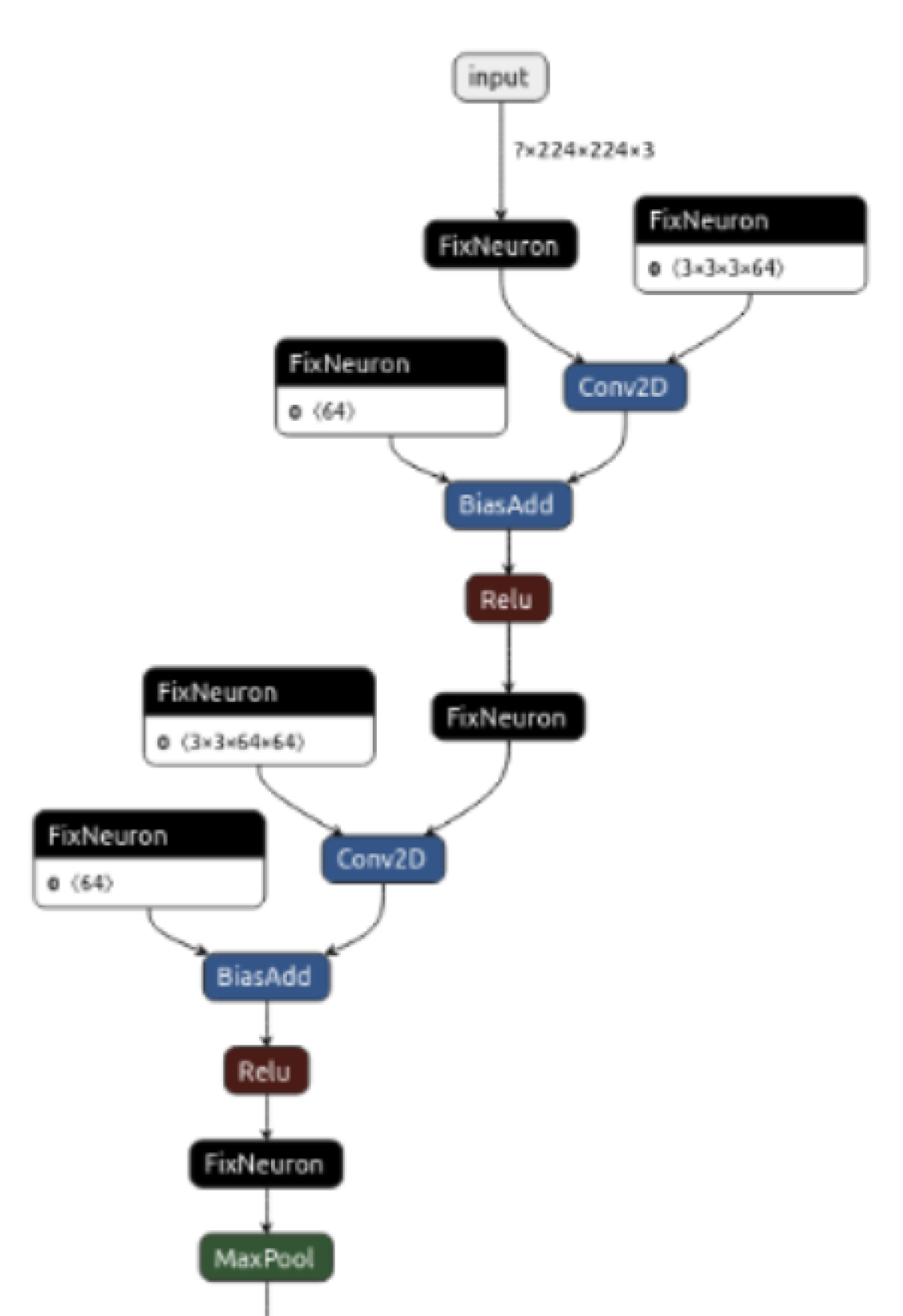
Figure 1: VGG 16 first three layers: Conv1+Relu + Conv2+Relu + MaxPool

In general, we have a tensor as input, say an image. We have multiple outputs: an image and annotations. We represent the computation by a direct acyclic graph (DAG). A node represents a computation with multiple inputs and a single output. We separate inputs and parameters. Parameters are constants and not computed: they are read (once) and from a dedicated memory space. Each node has a single output tensor and each node is connected by a path to both an input and an output node. Tensors are up to four dimensional vectors and they represent data and a memory space. A node is associated with a single output tensor (e.g., written once and read by many nodes) and at least one input tensor (e.g., written by a single node, unless the node is an input itself). The DAG and a topological ordered sequence of nodes, a schedule, represent a valid computation and a computation is a sequence of Static Single Assignment statements (SSA). A graph may have multiple inputs and multiple outputs, a graph node has at least one input and only one output.

In Figure 1, we present the netron graphical representation [14] of a enhanced and quantized tensorflow graph. We represent two convolutions and one maxpool. There are custom FixNeuron layers as quantization transformation layers for weights, biases, and for activation tensors so that to transform the original float arithmetic into 8 bits. Weight and bias are parameters and read only once. FixNeurons contain the information about range and precision of the result tensors and it is a quantization solution used within the Vitis framework [15]. Such a graph structure is integral part of the front end (i.e., quantization and it may involves re-training or fine tuning) it will assure that the computation can be carried on using 8bit arithmetic. Parameters and neurons are assimilated by the compiler into the corresponding node (i.e., convolution) in order to reduce the size of the graph and its complexity. Eventually, we reduce the 15 nodes to 4: 1 input, 2 convolutions, and 1 maxpool (and optimized to 3 by fusing convolution and maxpool). The schedule is shorter. These graph optimizations are standard nowadays and we do not dwell on them. Also, we assume that the DAG has operations we can reduce to basic FPGA operations (e.g., no softmax no tensor reshapes).

We present a recursive approach that divides/tiles the node operations in custom and optimized elementary instructions. The memory hierarchy and the schedule specify when and where tensors are computed and stored; this summarizes the memory foot print and memory pressure; in turn, the available space determines potential parallelism and feasible scheduling. The compiler has tools for the exploration of schedule and parallelism exploitation by splitting the graph into small enough convex sub-graphs (i.e., the sub-graph has no path exiting and re-entering the subgraph). We shall not present details about these tools at this time (you may find more details about memory allocation and schedule exploration in [16]). The elementary instructions are specific to the hardware thus we must present at least its abstraction.

III Hardware Abstraction

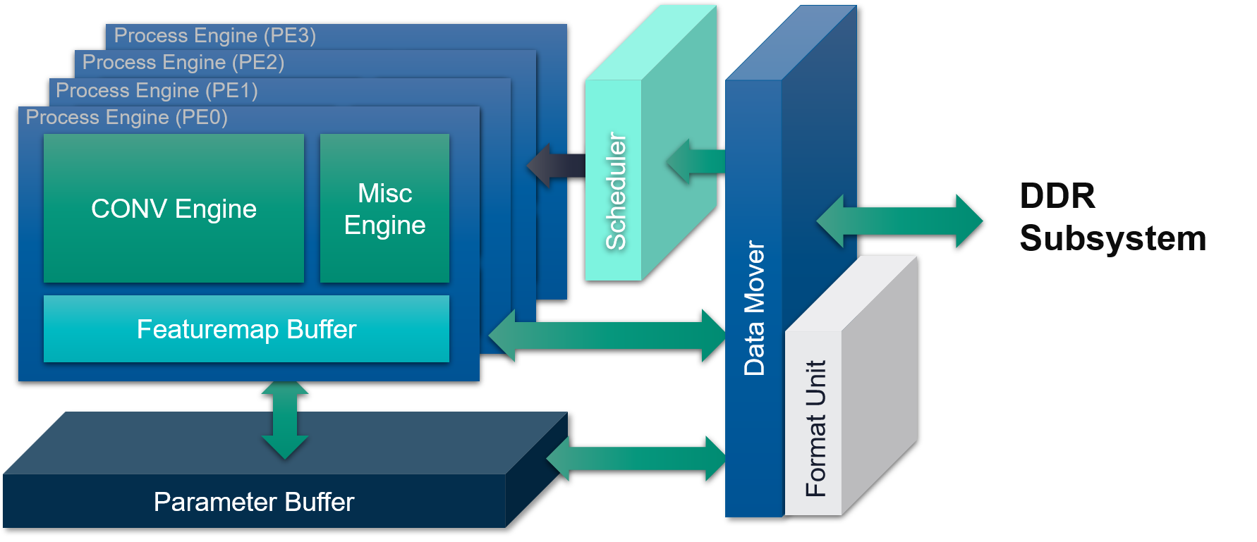
Figure 2: Basic HW abstraction

We present a graphical abstraction of the hardware in Figure 2. We have a main DDR memory where Inputs, Outputs, Parameters, and Instructions are stored. We have one main unit composed by four Process Engine (PE) and one Parameter memory (PM) for parameters. Every PE has a Feature map memory (FM) for input and output tensors and two computational engines: CONV and MISC. The PEs represent a Single Instruction Multiple Data (SIMD) architecture and it will work computing 4 tensors at any time (up to 16 concurrently on a U280). For compiler purposes, the code generation focus on a single PE and thus a single tensor computation, and only for data movement to/from DDR multiple tensors are involved (i.e., 4 tensors).

The memories PM, FM, and DDR are scratch pads. The compiler has the responsibility to manage allocation and de-allocation of every tensors. The PM and FM are circular buffers: that is a tensor can wrap around the last address back to the beginning and a tensor is stored contiguously. The circular property is necessary for streaming data to and from DDR where only a part of the tensor will be transient but contiguous and without overlapping. The DDR is not circular, we assume tensors will fit entirely, and it is logically split by register pointers into 5 parts: inputs, outputs, parameters, instructions, and swap/stack for memory data management (the equivalent of a compiler stack or malloc space). The architecture is more efficient for tensors with no small dimensions we call channels. The Format Unit is designed to change the layout of the inputs (images) on the fly to improve efficiency, due to the small number of 3 RGB channels (i.e., images and image classification). If the number of channels is larger than 8, the format unit is circumvented.

Every PE has a FM and four functional units (two shared). The FM is composed of three distinct circular memories with one read and one write port each; every memory is composed of eight banks that we can read and write them in parallel. The four functional units are:

• LOAD: This moves data from DDR to FM by means of a LOAD instruction. The same instruction can move parameters from DDR to PM.

• SAVE: This moves data from FM to DDR.

• CONV: This is a systolic array convolution engine: it reads the parameters from the common PM, the inputs and the outputs from its local FM.

• MISC: The miscellaneous unit is responsible for three types of operations: max pool, element wise addition, and data movement used for sample, up-sample, and identity. It reads and writes in its local FM.

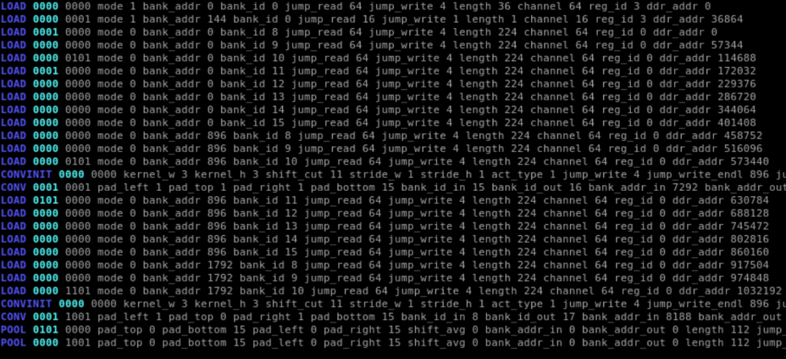
Figure 3: Sample of our human-readable code

There is a correspondent instruction for each unit: LOAD, SAVE, CONV, MISC (MAXPOOL and ELT). Each unit can execute in parallel and thus each instruction can be issued in parallel. Each instruction is synchronized by two entries: DPON and DBBY. DPON describes the operation types the current instruction depends on (multiple instructions). DPBY describes the operation types the current instruction depend by (multiple instructions). The dependency is by type only. An excerpt of generated code (without comments) is in Figure 3, and the first two entry of the instruction represent the instruction dependency DBON and DPBY (i.e., CONV DBON DBBY …). The specific value of the dependency encoding is immaterial at this time. However, if you are thinking about issuing instruction sequentially these attributes will be associated with the preceding and succeeding instruction in the schedule. This is easy. If you are thinking about parallelism, how to issues the instructions so that these dependencies will rely only on the type of the instructions is not that easy. The compiler cannot rely on when nor on the instruction number since issued instruction 0. For example, software pipelining is not straightforward. We shall return and explain this in Section VII.

IV Nodes and Computations

Consider a convolution operation ${\boldsymbol{Y}}={\boldsymbol{W}}{\otimes}{\boldsymbol{X}}+{\boldsymbol{B}}$, where ${\boldsymbol{X}}\in\mathbb{R}^{h_{i},w_{i},c_{i}}$, ${\boldsymbol{Y}}\in\mathbb{R}^{h_{o},w_{o},c_{o}}$, and ${\boldsymbol{W}}\in\mathbb{R}^{c_{o},h_{L},w_{M},c_{i}}$. The full definition is

$${\boldsymbol{Y}}\leftarrow{\dot{\sum}}_{i=1}^{h_{o}}{\dot{\sum}}_{j=1}^{w_{o}}{\dot{\sum}}_{k=1}^{c_{o}}\\ \sum_{l=1}^{h_{L}}\sum_{m=1}^{w_{L}}\sum_{n=1}^{c_{i}}x_{(i+l-1,j+m-1,n)}w_{(k,l,m,n)}+b_{k}\large$$ (1)

Any activation tensor has three main dimensions: the channel $c_{i}$, which is the innermost; the width $w_{i}$, which is the middle one; and the height $h_{i}$, which is the outermost. The tensor is stored in memory following the same logic. Here, we omit any batch size reference.

Each element of the ${\boldsymbol{Y}}$ tensor is the following computation based on summations:

$$y_{(i,j,k)}=\sum_{l=1}^{L}\sum_{m=1}^{M}\sum_{n=1}^{N}x_{(i+l-1,j+m-1,n)}w_{(k,l,m,n)}+b_{k}$$ (2)

We refer to this computation as a convolution. A convolution is defined as a 6 dimensional loop, Equation 2, represents the innermost loop and the outer loop is three iteration loop

$${\boldsymbol{Y}}\leftarrow\dot{\sum}_{i}^{h_{o}}\dot{\sum}_{j}^{w_{o}}\dot{\sum}_{k}^{c_{o}}y_{(i,j,k)}$$ (3)

From here on, we will not specify $\dot{\sum}$, that is an iterative loop, and use the $\sum$ symbol everywhere; any misunderstanding will not be harmful and the formulation concise. The computation will go from right to left and we write the formulae from left to right.

The process of thinking of ${\boldsymbol{W}}{\otimes}{\boldsymbol{X}}+{\boldsymbol{B}}$ as a single operation like a loop, partitioning it into smaller loops, and then reconstruct as a unfolded sequence of basic convolutions is a useful one. We use a declarative expression using loops to show the details of the computation and express the division of the computation. Programmatically, the recursive nature is simpler to use. In our heads, when we talk about tiling we mean recursion. In our framework, there is no Loop construct, and a computation is a tree where each leaf is a single computation summarized by a few HW instructions and inner nodes represent sub-computations (and data movements). However, recursion makes a poor presentation tool to the compiler community at large where iterative loops are dominant. Clearly, having 9 or more loops as code description will give too much information and will be cumbersome. We decided for presentation sake that will play with a mixed representation to keep the iterative nature of the computation and the recursive division and code generation (to keep it short). Hopefully, the mixed approach will strike an advantageous compromise (or make everybody unhappy).

V The Recursive Description of a Computation (into Computations)

A techincal distinction is in order. A node in the DAG is a fully defined computation and it is atomic. The main point to realize is the computation of a node is a function of the context in a DAG (this is obvious). For a node computation, the input addresses and the output address are specified, the properties of the node like stride and padding are associated to the computation. However, if we can divide the computation into components, each component is a computation that may have different attributes (i.e., padding) and access input and outputs with patterns that are not the same of the original. For example, let us consider Equation 2, the order of the loops determines the input access patterns, the sub computation may have to exploit different ones from the original.

The recursive description of code generation follow this idea from the largest to the smallest problem: We split the computation by width, by height, and last by weights. We present the process using convolutions but the same idea apply for all computations (well not the weight decomposition)

V-A W-splitting: overlapping inputs

Consider again the convolution computation: ${\boldsymbol{Y}}={\boldsymbol{W}}{\otimes}{\boldsymbol{X}}+{\boldsymbol{B}}$ with unitary stride, no padding. We split the tensor ${\boldsymbol{Y}}$ in two parts by the width dimension ${\boldsymbol{Y}}_{i=1\equiv[1,a]}$ and ${\boldsymbol{Y}}_{i=2\equiv[a+1,w_{o}]}$:

$${\boldsymbol{Y}}={\boldsymbol{Y}}_{1}|{\boldsymbol{Y}}_{2}=\sum_{v=1}^{2}{\boldsymbol{Y}}_{v}$$ (4)

To perform the computation we need to split the input vector into two parts partially overlapping:

$${\boldsymbol{X}}={\boldsymbol{X}}_{w_{i}\in[1,(a-1)+L]}|{\boldsymbol{X}}_{w_{i}\in[a,w_{i}]}$$ (5)

There is an overlap if $L>1$, see Figure 4

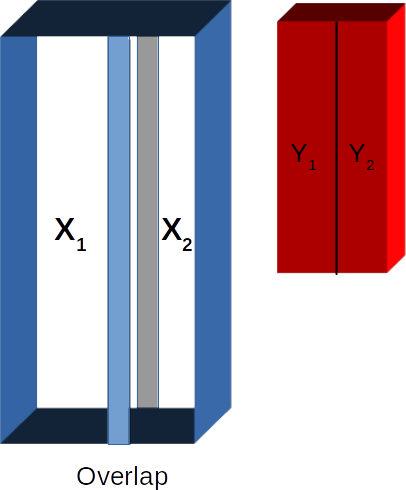
Figure 4: W-Splitting with input overlap azure band between $X_{1}$ and $X_{2}$

$${\boldsymbol{Y}}=\sum_{v=1}^{2}{\boldsymbol{W}}{\otimes}{\boldsymbol{X}}_{v}+{\boldsymbol{B}}$$ (6)

If there is a stride $s_{w}$ and padding $p_{w}$:

$${\boldsymbol{X}}={\boldsymbol{X}}_{w_{i}\in[1,(a-1)s_{w}+L]}|{\boldsymbol{X}}_{w_{i}\in[a*s_{w},w_{i}]}\\$$ (7)

$${\boldsymbol{X}}={\boldsymbol{X}}_{w_{i}\in[1,(a-1)s_{w}+L-p_{w}]}|{\boldsymbol{X}}_{w_{i}\in[a*s_{w}-p_{w},w_{i}]}$$ (8)

The complete formulation is cluttered, we shall omit it for simplicity whenever possible. Consider a tensor of size $1\times w\times c$, our hardware has a few requirements about the size of this simple size tensor. If we say that $\gamma$ is $\max(w*c)$ for which we can read and perform operation on the tensor, we split the computation so that

$${\boldsymbol{Y}}=\sum_{v=1}^{\lceil\frac{w*c}{\gamma}\rceil}{\boldsymbol{W}}{\otimes}{\boldsymbol{X}}_{v}+{\boldsymbol{B}}$$ (9)

The data dependency between the input and the output (by the weight tensor shape) forces an overlapping space between iterations. As a matter of fact, the computations are independent and Equation 4 shows this is the first recursive level and it is possible only if either input or output have $\max(w*c)\geq\gamma$. Longer vector in the width dimension will take more space. Thus less space to perform double buffering using the maximum parallelism of the architecture. The W-Splitting is the classic loop tiling only that tiles share inputs points, tensors are meant to be in DDR, $X_{1}$ and $X_{2}$ are scattered in DDR, but otherwise vectors will stream well in FM memory where they will be contiguous: The H-Splitting is tiling and software scheduling so that to optimize data streaming and architecture parallelism.

V-B H-Splitting

As usual, we consider ${\boldsymbol{W}}{\otimes}{\boldsymbol{X}}+{\boldsymbol{b}}$ with ${\boldsymbol{Y}}\in\mathbb{R}^{h_{o},w_{o},c_{o}}$. We have a preferred computation height $H_{C}=8$ for convolution ($H_{E},H_{P}=2$ for addition and pool). This means: first, we have a preference in producing an output tensor with height $H_{c}$; second, smaller dimension are possible but less efficient; third, the tiling is function of the operation type (and if they are fused, not straightforward). If ${\boldsymbol{Y}}_{v}$ means $y_{i,*,*}$ with $i\in[(v-1)H_{c}+1,vH_{c}]$ then we can use the previous notation to describe the computation:

$${\boldsymbol{Y}}=\sum_{v=1}^{\lceil\frac{h_{o}}{H_{c}}\rceil}{\boldsymbol{Y}}_{v}=\sum_{v=1}^{\lceil\frac{h_{o}}{H_{c}}\rceil}{\boldsymbol{W}}{\otimes}{\boldsymbol{X}}_{v}+{\boldsymbol{B}}$$ (10)

The minimum output foot print is $(H_{c},W_{o},C_{o})$, the input has foot print with stride $s_{h}$ and hernel $k_{h}$

$$Size({\boldsymbol{X}}_{v})=((H_{c}-1)*s_{h}+k_{h},W_{i},C_{i})$$ (11)

If the minimum foot print does not fit any of the memories in FM, we shall reduce $H$ accordingly. Of course, smaller $H$ will produce less efficient computations and slower executions. At this stage, we reformulate the computation so that we have $\frac{h_{o}}{H_{c}}$ convolutions and each will compute a $H_{c}$-tall output tensor. If reducing the height to one is not enough, we must w-split the computation first.

As you can see, W-Splitting and H-Splitting are very similar. There are a few differences:

1. The W-splitting is triggered by the number of available rows in the feature-buffer banks (FM)

2. The H-splitting is triggered by the number of banks in FM and the computational parallelism.

3. H-Splitting will not have input overlap (we shall explain further) by exploiting streaming and computational parallelism.

VI Operation Fusion

Our HW can perform in parallel pool and convolution operations. For inference network it is common to fuse convolution and pool operations into a single operation. In previous architectures, the main idea is to reduce the memory pressure by removing the need of the intermediary tensor (by using a smaller and temporary one). In this architecture we are actually do fusion to exploit instruction parallelism and data streaming.

$${\boldsymbol{Y}}={\bf MaxPool}({\boldsymbol{T}}={\boldsymbol{W}}{\otimes}{\boldsymbol{X}}+{\boldsymbol{b}})$$ (12)

where using the summation as a loop:

$$Y_{i,j,k}=\sum_{n=1}^{k_{w}}\sum_{m=1}^{k_{h}}max((T_{i+m-1,j+n,k})$$ (13)

We can tile by the usual height but the maximum height is $H_{p}=2$

$${\boldsymbol{Y}}=\sum_{v=1}^{\lceil\frac{h_{o}}{H_{p}}\rceil}{\bf MaxPool}({\boldsymbol{T}}_{v})$$ (14)

The output sub-tensor will have foot print $(H_{p},w_{o},c_{o})$, the intermediary tensor, which is the output of the convolution, has a foot print:

$$(T_{h}=(H_{p}-1)*PoolStride_{h}+PoolKernel_{h},W_{t},C_{t})$$ (15)

and the input

$$((T_{h}-1)*ConvStride_{h}+ConvKernel_{h},W_{i},C_{i})=\\ (((H_{p}-1)*PS_{h}+PK_{h}-1)*CS_{h}+CK_{h},W_{i},C_{i})$$ (16)

$${\boldsymbol{Y}}=\sum_{v=1}^{\lceil\frac{h_{o}}{H_{p}}\rceil}{\bf MaxPool}(\sum_{w=1}^{\lceil\frac{h_{t}}{H_{c}}\rceil}({\boldsymbol{W}}{\otimes}{\boldsymbol{X}}_{w}+{\boldsymbol{b}})_{v})$$ (17)

$${\boldsymbol{Y}}=\sum_{w=1}^{\lceil\frac{h_{t}}{H_{c}}\rceil}\sum_{v=1}^{\lceil\frac{H_{c}}{H_{p}}\rceil}{\bf MaxPool}(({\boldsymbol{W}}{\otimes}{\boldsymbol{X}}_{w}+{\boldsymbol{b}}))$$ (18)

Equation 18 describes how the fusion operation works at steady state. The formulation do not consider prologue nor epilogue, there is no description of the effects of padding for input or temporary space. Clearly, it shows that instead of two passes as in Equation 17, we have one pass of the input and of the output and two computation stages.

Operation fusion has the side effect to create tensors of different sizes and there is a multiplicative factor as a function of the stride computation. If the tile has to be reshaped to accommodate smaller footprints, less efficient computations are required and we turn off fusion. The same idea applies with little or no modification to

$${\boldsymbol{Y}}={\boldsymbol{W}}{\otimes}{\bf MaxPool}({\boldsymbol{X}})+{\boldsymbol{b}}$$ (19)

We call the steady state of the computation the number of convolution output $H_{c}$ and the max pool output $H_{p}$. In practice, this is an application of discrete mathematics: we have a valid steady state if we can consume the convolution points at the same rate we can produce them. That is, it exists a $k$ so that $kH_{p}=H_{c}$ and the intermediate computation fits in memory.

In summary: W-Splitting, H-Splitting and fusion

$$\begin{split}{\boldsymbol{Y}}=&{\bf MaxPool}(({\boldsymbol{W}}{\otimes}{\boldsymbol{X}}+{\boldsymbol{b}}))\\ &\sum_{v=1}^{\lceil\frac{w_{i}}{\gamma}\rceil}{\bf MaxPool}(({\boldsymbol{W}}{\otimes}{\boldsymbol{X}}_{v}+{\boldsymbol{b}}))\\ &\text{ a.k.a. W-Split}\\ &\sum_{v=1}^{\lceil\frac{w_{i}}{\gamma}\rceil}\sum_{k=(v-1)*\gamma+1}^{v*\gamma}{\bf MaxPool}({\boldsymbol{T}}_{k}=({\boldsymbol{W}}{\otimes}{\boldsymbol{X}}_{v}+{\boldsymbol{b}}))\\ &\text{ a.k.a. W-Split + fusion }\\ &\sum_{v=1}^{\lceil\frac{w_{i}}{\gamma}\rceil}\sum_{k}\Big{(}\sum_{h=1}^{\lceil\frac{h_{t}}{H_{c}}\rceil}\sum_{v=1}^{\lceil\frac{H_{c}}{H_{p}}\rceil}{\bf MaxPool}(({\boldsymbol{W}}{\otimes}{\boldsymbol{V}}_{h}+{\boldsymbol{b}}))\Big{)}\\ &\text{ a.k.a. H-Split + fusion}\\ \end{split}$$ (20)

The notation becomes heavy, incorrect, difficult to read and to understand. We will not indulge further notation describing W-Split and H-split. The power of operation fusion is really evident when we combine H-Splitting, operation fusion, and software pipelining.

VII Software Pipelining as Code Reorganization

Consider a node computation ${\boldsymbol{Y}}={\bf MaxPool}({\boldsymbol{T}}={\boldsymbol{W}}{\otimes}{\boldsymbol{X}}+{\boldsymbol{b}})$ where the input data is in DDR and the output data will be in DDR, also consider the case where the PM can fit the weights. The operation is fused and represented by

$${\boldsymbol{Y}}=\sum_{w=1}^{\lceil\frac{h_{t}}{8}\rceil}\sum_{v=1}^{\lceil\frac{8}{2}\rceil}{\bf MaxPool}(({\boldsymbol{W}}{\otimes}{\boldsymbol{X}}_{w}+{\boldsymbol{b}}))$$ (21)

As a short and abstract description, the code for the computation above:

$${\bf Op}({\boldsymbol{X}})=\sum_{i=1}^{\lceil\frac{h_{t}}{8}\rceil}T_{i}\text{ and }T_{i}=L_{i}C_{i}P_{i}S_{i}$$ (22)

As a practical example for the first full computation of Convolution and Pool:

$$\begin{split}T_{1}=&L_{1}C_{1}P_{1}S_{1}\\ L_{1}=&\sum_{\ell=1}^{12}LOAD_{\ell}\text{, read 12-high vector}\\ C_{1}=&\sum_{c=1}CONV_{c}\text{, 1 conv, 12 inputs, 8 outputs }\\ P_{1}=&\sum_{p=1}^{4}POOL_{p}\text{, 4 pool, 8 inputs, 4 outputs}\\ S_{1}=&\sum_{s=1}^{4}SAVE_{s}\text{, 4 saves}\end{split}$$ (23)

In general for $T_{i}$ and clearly visible in the particular $T_{1}$ instruction, each sub-computation has a different length of instructions: 12, 1, 4, and 4 respectively. Also the execution time of each sub computation is also function of the efficiency, shapes, and size of the operations, and thus a function of how we split the computation in parts. This is not a classic Very Long Instruction Word (VLIW) although we want to exploit instruction level parallelism (it is not VLIW because our different execution time of each sub-computation implies that issuing the long instruction is not enough to support their correct queuing and execution).

The tiling will split the computation into a sequence of basic computations: because each tile has input data in DDR, the first operation of the tile will be a load, then the main computation such as convolution and pool (if it is a fused operation), and it will conclude with a save instruction in order to move the data back into DDR. In a practical context, each $L_{i},C_{i},P_{i},$ and $S_{i}$ are a sequence of instructions not necessarily a single instruction.

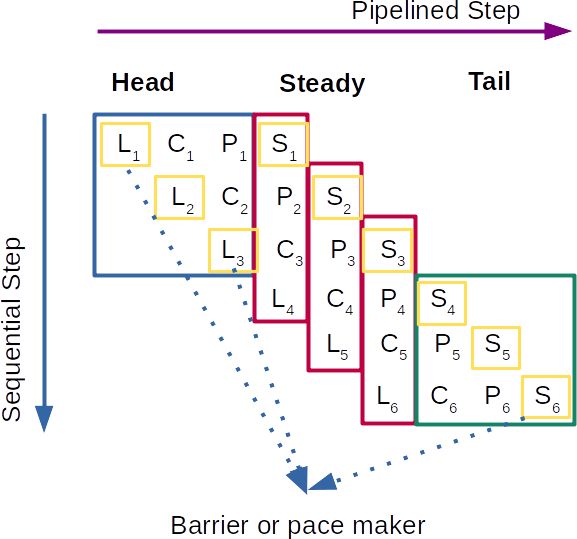
Figure 5: Compiler software pipelining

As a reminder of the meaning of the our notation in Equation 22: we imply a strict dependency within the $T_{i}$ computation and we imply a dependecy from $T_{i}$ and $T_{i+1}$:

$$L_{1}\rightarrow C_{1}\rightarrow P_{1}\rightarrow S_{1}\rightarrow L_{2}\rightarrow C_{2}\rightarrow P_{2}\rightarrow S_{2}...$$ (24)

Thus the computation is purely sequential. The goal of software pipelining is to unlock the parallelism from instruction $T_{i}$ and $T_{i+1}$.

The way we presented our computation in Section V, we have the property that close-by tiles work on close-by data ($i$ and $i+1$) and they can stream into memory quite naturally. This has the property that if we can exploit instruction parallelism we need just to explore direct neighbors tiles so that to have the least memory foot print. To exploit the parallelism we must reorganize the computation differently and work on the dependencies.

$${\bf Op}({\boldsymbol{X}})=Head+(Steady=\sum_{i=4}^{k}L_{i},C_{i-1},P_{i-2},S_{i-3})+Tail$$ (25)

where

$$Head=L_{1}+(L_{2}+C_{1})+(L_{3}+C_{2}+P_{1})$$ (26)

This means that $L_{1},L_{2},L_{3}$ are barrier instructions so that $C_{1}$ is parallel to $L_{2}$ and it can start only after $L_{1}$; $L_{3}$ will start only after $L_{2}$ and $C_{1}$ are done. Also notice that by the end of the Head computation we have three live tensors $L_{3}$, $C_{2}$ and $P_{1}$ that can be stored into a different FM.

$$Steady=\sum_{i=4}^{k}(L_{i},C_{i-1},P_{i-2},S_{i-3})$$ (27)

$S_{1}$ will start only after $L_{3},C_{2},P_{1}$, and $S_{2}$ after $L_{4},C_{2},P_{2},S_{1}$. The $S_{k}$ are barrier or pace maker instructions. The parentheses are used for emphasis to show that the instructions within are parallel. The save operation $S_{j}$ is the only operation that will free space (in the common sense). At steady pace, we can see the parallel nature of the instruction issuing and that we are performing a natural double buffering for each instruction. Take another look at Figure 5 and in particular at the instructions in red: $S_{i}$ instructions read contiguous sub-tensors and write them, in practice only $S_{i}$ and $S_{i+1}$ need to be alive at the same time to make sure the computation is coherent and correct. This is true for the other operations.

$$Tail=(C_{k}+P_{k-1}+S_{k-2})+(P_{k}+S_{k-1})+(S_{k})$$ (28)

Again $S_{k-2},S_{k-1},S_{k}$ are barriers and we can do that by the proper use of DPBY and DPON:

$$L_{i}+C_{i-1}+P_{i-2},S_{i-3}:DPBY\rightarrow S_{i-2}$$ (29)

$$L_{i}+C_{i-1},P_{i-2},S_{i-3}\leftarrow S_{i-2}:DPON$$ (30)

This is the basic idea of software pipelining for other architectures and compilers: the main difference is we handle a sequence of instructions instead of a single instruction common for long vectorized instructions. Each instruction has different execution time, the starting time is not assured by issuing the instruction but the starting is function of the issuing of the previous instructions, and synchronization with previous instructions is by type and thus by DPBY and DPON events. Still the encoding of the dependency is immaterial. If the memory space is a circular buffer, there is not data overlapping.

Notes: Software pipelining and circular buffers create a streaming computation, a software driven streaming computation. The barriers must change between the head computation and the rest because by construction the $L_{i}$ will not be present in the tail and they may be finished during the steady computation. There are corner cases where we must introduce No-Operation bubble in the stream computation. No-Op is a place holder for an instruction that is no necessary anymore for the computation but it is necessary for the smooth code generation. The arguments here presented do not rely on the order and length of the computation $T_{i}$; that is, $T_{i}=L_{i},P_{i}$ will work as above and it will exploit parallelism between $L_{i}$ and $P_{i}$.

VIII Transpose convolution: optimal implementation

We know that the transpose convolution, known as deconvolution, is equivalent to the sequence of an optional upsample and a convolution. For our architecture, this is the only way to compute a deconvolution. When there is an upsample, this means that the input of the following convolution has lots of zeros. We avoid the zero computation by reorganize the deconvolution into a set of convolutions. In practice, we have a fully automated Deconvolution = Convolutions transformation.

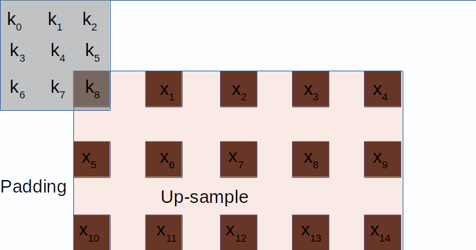
Figure 6: Deconvolution= Upsample 2x2, Padding 2, kernel 3x3

We describe the main idea by visualizing it for a deconvolution that can be computed by a upsample 2x2, padding of 2, and a convolution with kernel 3x3 and stride one. See Figure 6. If we run the kernel, from the top left corner to the right, we see that the first output is just the contribution input $x_{0}$ and $k_{8}$, The second output is the contribution of $x_{0}$ and $k_{7}$, and the the third output is $x_{0}*k_{6}+x_{1}*k_{8}$. If we move the kernel one level below and then to the right, we have $k_{5}*x_{0}$, $k_{4}*x_{0}$ and $k_{3}*x_{0}+k_{5}*x_{1}$. Now let us take a look at Figure 7

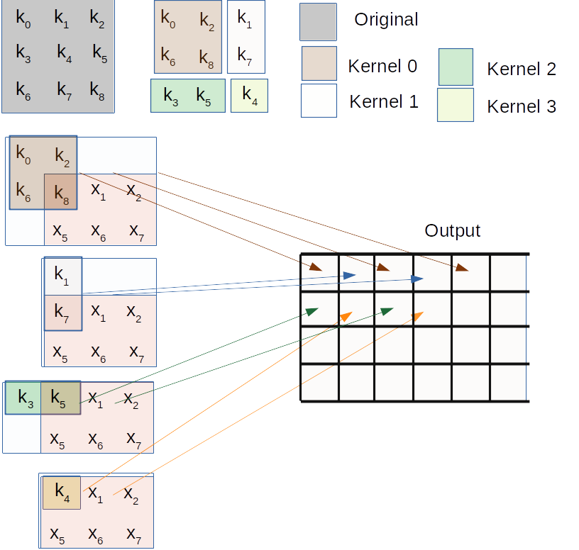
Figure 7: Convolution Series = Deconvolution

We can see that if we avoid to upsample the input and we reduce the padding by 1, we can compute the same elements as before. We take $Kernel_{0}$, we set on the top left and the first output is $x_{0}*k_{7}$, if we move the kernel by one spot to the right we have $k_{6}*x_{0}+k_{8}*x_{1}$ and this is the third output. So if we move $Kernel_{0}$ we compute output $0,2,4,...$. If we take $Kernel_{1}$ and we do not pad left, we can compute output $1,3,5,..$. We take $Kernel_{2}$, we do not pad the top of the input and we move the kernel to the right and we compute the second row outputs $0,2,..$. Eventually we do not pad the input and we use $Kernel_{4}$ to compute $1,3,5,...$ of the second row. We skip the details about the bottom and right padding for all kernels because we need to do some book keeping and instead of clarity we achieve likely the opposite.

The pictures above should be able to convince that the original computation and the series of convolutions are equivalent. We need to describe how we can systematically determine the kernels so that we achieve such a property. The simplest way to visualize how the sub-kernels are cut is by the overlapping of the original kernel and the upsample input, like in Figure 8 but we do not need to move the kernel around so much.

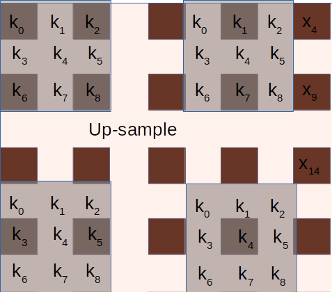
Figure 8: Kernel determination = Original kernel and upsample pattern

Given a kernel $k\times k$ and an upsample $m\times m$, there are $m-1$ zeros, the number of kernels is $\min(k,s)^{2}$. One way to see this intuitively, if $s=2$, the number of subkernels cannot be more than 2 for any $k$. Here, we shall work with only upsample 2x2, and thus the original kernel will be replaced by 4 subkernels. In this section, we have the most variety as shape and size. For example, for a kernel 4x4, we shall have 4 kernel 2x2.

The compiler allows to have a transpose convolution implemented as $(2\times 2)$-Upsample + $k\times k$-Convolution or as 4 $(k-1)\times(k-1)$ convolutions.

$$DECONV_{k,s,p}(X)=CONV_{k}(Padding_{p}(Upsample_{s}(X)))$$ (31)

$${\boldsymbol{W}}{\otimes}Pad(Usample({\boldsymbol{X}},s),p)+{\boldsymbol{b}}$$ (32)

Pad is not an instruction, Upsample is a combination of MISC and LOAD operations. The Upsample + convolution can be split and fused and we can exploit software pipeline as in Equation 33

$$\sum_{v=1}^{\frac{H}{8}}\sum_{w=1}^{8}{\boldsymbol{W}}{\otimes}Pad(Usample({\boldsymbol{X}}_{w},s),p)+{\boldsymbol{b}}$$ (33)

If we use the sequence of convolutions

$$\sum_{v=1}^{\frac{H}{8*2}}\sum_{k=1}^{4}{\boldsymbol{W}_{k}}{\otimes}Pad_{k}({\boldsymbol{X}}_{v})+{\boldsymbol{b}}$$ (34)

The equation is taking many liberties so that we can be concise. The factor $8*2$ is because convolution has optimal output by $H_{c}=8$, but there are 2 vertical kernels such as $Kernel_{0}$ and $Kernel_{3}$. We may have to reduce the $H_{c}$ to make sure we can compute the output into feature map buffer. The size of ${\boldsymbol{X}}_{v}$ is similar to the one for regular convolution but not exactly: here we require some book keeping and details will make the formulation confusing.

As today, our architecture does not allow strided outputs by row, so we need to perform the convolutions and then shuffle them by row

$$\sum_{v=1}^{\frac{H}{8*2}}\sum_{k=1}^{4}{Shuf}({\boldsymbol{W}_{k}}{\otimes}Pad_{k}({\boldsymbol{X}}_{v})+{\boldsymbol{b}}))$$ (35)

The shuffle is based on Element wise operations and thus can be done in parallel with the convolution. So we keep the advantage of a minimum number of computations and the formulation is symmetric to the original Upsample + Convolution.

To show optimality: the series of convolution is a complete partition of the original kernel without repetition. So every term in Equation 34 is computed in Equation 31 as well, however there is no zero computations and it cannot be done with any fewer computations (without changing the definition or the computation).

IX Compiler Organization

The compiler follows an organization similar to other compilers in the field and within Xilinx’s open software projects.

1. We parse a network into an intermediate structure XIR composed by Op and Tensor classes (from Caffe, TensorFlow, and XModel –XIR)

2. We create a Hyper Graph (V,E) where a node in V is a (Op,Tensor) pair. The Hyper Graph is designed so that the compiler can

   • explore different schedules

   • introduce operation fusion at graph level

   • determine input and output nodes (thus interface)

   • cut and reorganize the graph (i.e., debug)

   • add nodes (i.e., memory coherence)

3. We redirect parameters to be constants instead of operands

4. We enrich the tensors with quantization information: quantization information is associated with range, like $(-8,8)$ and minimum interval between two consecutive number in the range.

5. We perform graph manipulations in order to keep the minimum number of nodes.

6. Optional, we explore operation parallelism by scheduling and memory space estimation.

7. For every Schedule until success:

   • we assign memory properties such as data memory layout

   • we determine when and if operation fusion can be done efficiently

   • we determine the memory allocation and reuse of inputs/outputs and parameters

   • we identify the nodes where we can perform parameters prefetching into PM.

   • we start the code generation of the primary computation by our recursive code generation

   • streaming and software pipelining

Given a graph, the compiler creates two outputs: the instruction set and the layout of the parameters in memory. We estimate and validate the instruction dependency. The compiler can be a standalone entity. In practice, it is used in combination with a partitioner: the main graph is split and any subgraph related to our architecture is the input to the compiler. The partitioner takes the output and annotates the subgraph with code and parameters in binary format. The run-time executes the partitioned graph (we will expand when showing performance of the model zoo).

X Experimental Results

We present a graphical representation of the execution by an HW simulator and the FPGA execution runs confirm the total execution time accuracy (i.e. Figure 9). Given the assembly code, it presents the execution time of each instruction and it shows the schedule and its execution. The architecture has four queues:

• LOAD: weight and activation tensors move from DDR to FM (blue) and to PM (black). The Figure represents the execution time for the transfer by color accordingly.

• MISC: the operation maxpool (green) and Element wise one or two operands (yellow).

• CONV: operations like initialization (red) and convolution (purple)

• SAVE: data movement from FM to DDR (purple).

The x-coordinate has double duties: it represents when an hw instruction is issued and the thickness of the line tells the duration. The x-coordinate represents time. The tools actually allows to use a mouse interaction to inspect each operation.

As practical comparison, we present the performance of our previous and current state of the art FPGA implementation for latency [16].

X-A Resnet 50

Figure 9: Compiler Resnet Timing

Figure 9 presents the visualization of Resnet50 assembly code generated by the compiler. This network is a reference and every HW must do well. Briefly, the network expose the following two basic optimizations:

$${\boldsymbol{Y}}={\bf MaxPool}({\boldsymbol{T}}={\boldsymbol{W}}{\otimes}{\boldsymbol{X}}+{\boldsymbol{b}})$$ (36)

and

$${\boldsymbol{Y}}=({\boldsymbol{W}}{\otimes}{\boldsymbol{X}}+{\boldsymbol{b}})+{\boldsymbol{Z}}$$ (37)

with an explicit fusion operation will exploit parallelism between convolution, pool, and element wise addition

$${\boldsymbol{Y}}=\sum_{i=1}^{H/H_{c}}(ELTWISE({\boldsymbol{W}}{\otimes}{\boldsymbol{X}}+{\boldsymbol{b}})_{H_{c}},{\boldsymbol{Z}}_{H_{c}})$$ (38)

In Figure 9, The first computation is a fused pipelined convolution and maxpool where the input is in DDR. We can see how the loads (light blue), convolutions (purple), and pool (green) instructions are scheduled. Then there are two element wise addition and convolution fusion and pipelining. At about the 1000 micro second mark we can see the lag because of tail computation. The compiler at this time will not start the next convolution because the output tensor is not completely computed. At the 6000 microsecond mark, we notice that

$$({\boldsymbol{W}}_{T}{\otimes}{\boldsymbol{X}})_{H}+{\boldsymbol{b}}_{T}$$ (39)

the compiler deploys the weight tiling and software pipelining: the weights do not fit the PM memory and weight load instructions (black) are pipelined with the convolution instructions.

The best performance we could achieve for resnet previously is 3.2ms for one image [16]. The estimated and practical execution time is 8.2 msec. The computation reach till the AVGPOOL computation and it has a throughput of 4 images. The hand optimized code is 7.5ms, Figure 10.

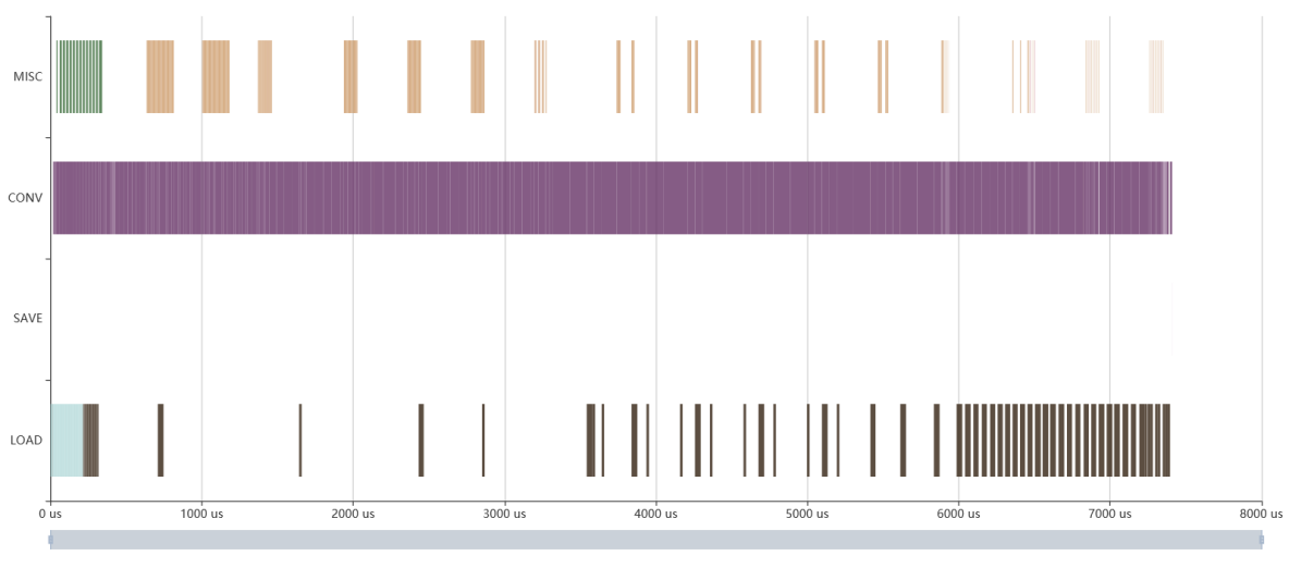
Figure 10: Expert Resnet Timing

As note, the hand tuned computation allows to starts the computation of layers before the predecessor completion, because accurate timing and clever use of circular buffers. Also a few max pools are removed from the computation altogether by recognizing optimizations available by the following 1x1 convolutions. The compiler does not deploy such a specific optimizations because they are applicable only on this resnet50.

X-B Inception v1

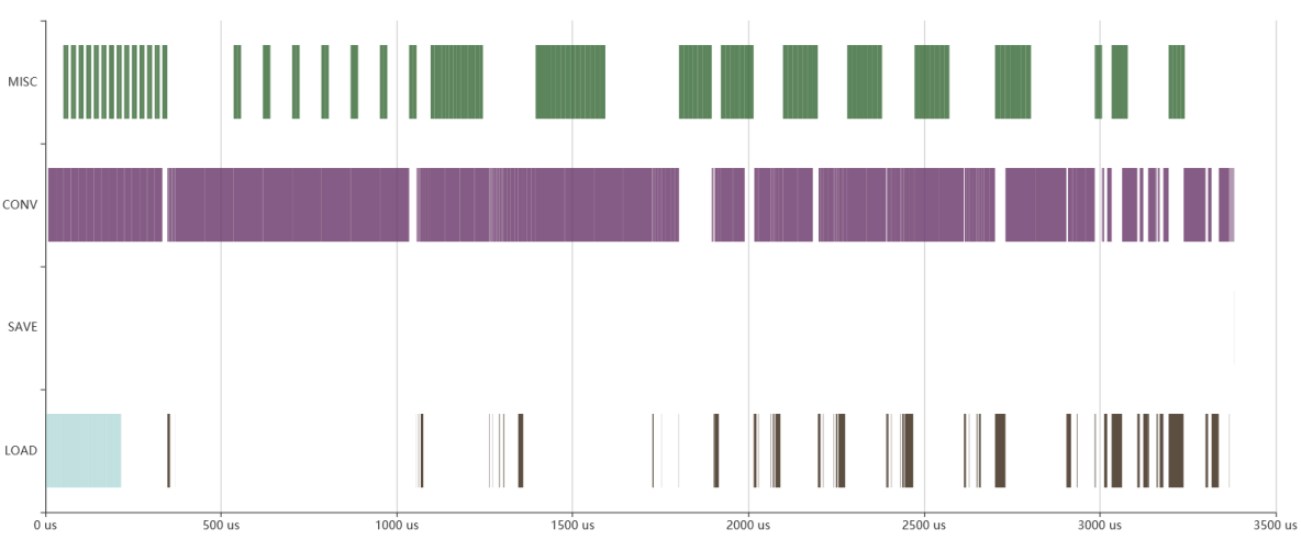
Figure 11: Inception v1 Timing

Inception V1 is an example where concatenation-concatenation sections of the network present two types of instruction parallelism. We can execute in parallel a maxpool and a convolution, or a fusion of convolution and maxpool (Equation 19). Although, parallel node level instructions are preferable when possible (i.e., no head and not tail warm up and cool off), we exploit a simple heuristic. If the following convolution is the largest among the one we could compute in parallel and the fusion allows a faster implementation, we fuse the operations. Otherwise, we keep them separated and let the scheduler seek for parallel schedule if possible. At mark 1500 microsecond, we can see a successful parallel scheduling. If you wonder about the pool (green) instructions at about 2000 microsecond, the max pool is a bottle neck of the computation and we do not try to move it.

We can achieve 4 images every 3.4 ms, in our previous implementation we achieve 1 image every 1 ms.

X-C Yolo v3

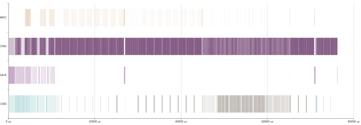
Figure 12: Yolo V3 Timing

Yolo V3 has element-wise operation and concatenation instructions to join different computation paths together (the combination of inception and resnet). As previous networks, the last part of the computation is weight heavy and the beginning is input/output heavy. Differently there is more stress about memory allocation and data movements. We need to use DDR as a swap space. Also a main difference is that the size of the outputs is larger than the inputs.

We can compute 4 images every 77 ms.

X-D VGG 16 (tensorflow)

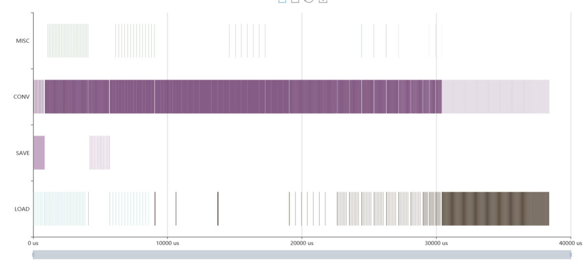
Figure 13: VGG 16

VGG is a long sequence of heavy convolutions, and this version ends the computation with three fully connected layers (FCs are ineffcient for this architecture).

We can compute 4 images every 37.3 ms for VGG-16 and 44.5ms for VGG-19, previously we could achieve 1 image every 18.2 ms and 20.5ms respectively (for the caffe version we could do better VGG16 1 image every 8.7ms using HW counters and 54ms considering the full runtime stack wall clock, [16]).

X-E Deconvolution and Cityscape

We start with a comparison of a synthetic deconvolution from a citiscape model.

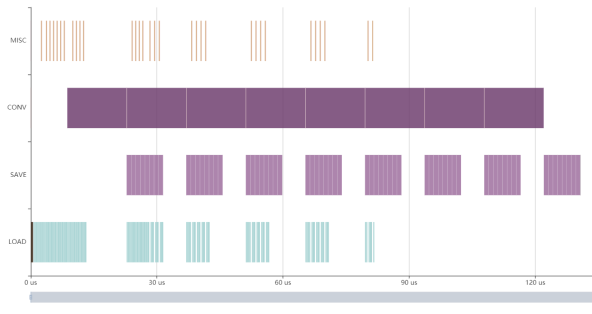
Figure 14: Deconvolution = Load (blue) + Upsample (yellow + blue) + Convolution (dark purple) + Save (light purple)

In Figure 14, we present the classic way to compute the deconvolution as a upsample and a Convolution. The estimated execution time by simulation is 0.130ms and the practical time is 0.55ms. The computation is convolution bound, this means that the convolution dominates the overall execution time. The upsample is a combination of data movement MISC operations and load from DDR, where we store zeros in advance. In DPUV3INT8 2.0 the upsample is implemented using only MISC instructions.

In Figure 15, we have the optimal implementation using only convolutions: the simulation time is 0.086ms and the practical time is 0.42ms. The computation is dominated by storing the result in DDR. These tests are single layer tests and thus reading and writing in DDR are mandatory. Nonetheless, the execution-time advantages are clearly measurable.

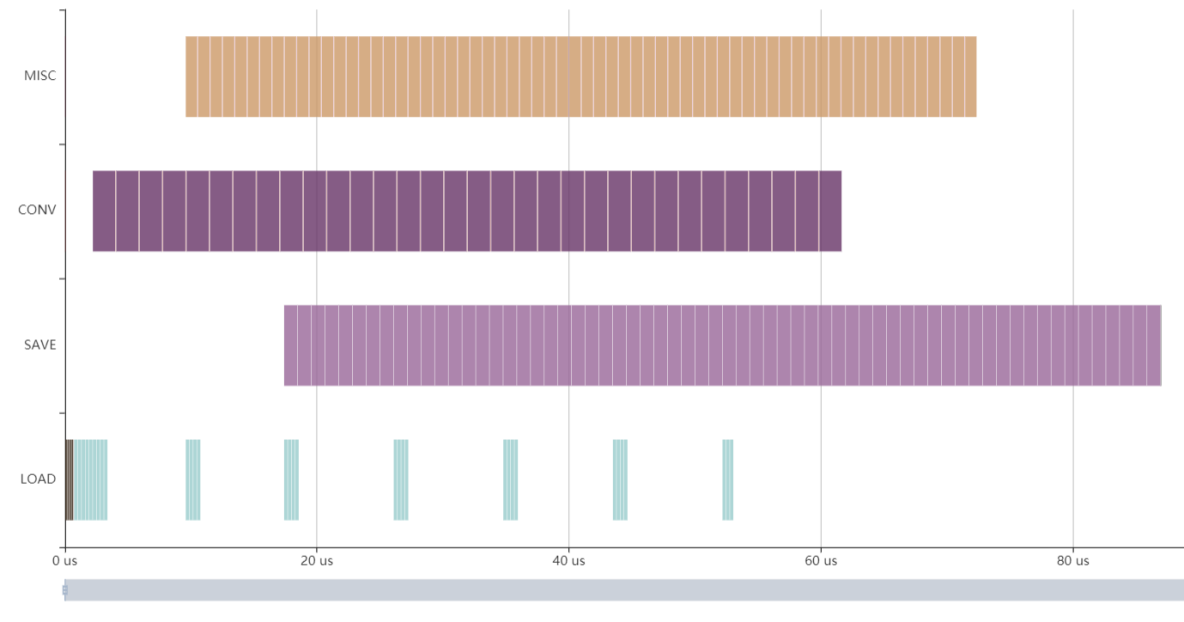
Figure 15: Deconvolution = Load (blue) + Convolutions (dark purple) + Shuffle (yellow ) + Save (light purple)

X-F Model Zoo

A model zoo is a collection of networks that is representative: it provides variety of applications that can be applied to a variety of hardware. This is a standardization. In particular, in the environment we work every model in the zoo is compiled–executed using a common interface. We call this interface xcompiler. The following models are available in Vitis and they can run and tested independently.

The xcompiler will take a model in native format, will create an intermediate representation XIR and applies a set of standard optimization passes. In short, a caffe model is transformed into a xmodel (XIR) that we call xnnc xmodel. The xnnc is the front end tool. The xcompiler takes the xnnc model and do optimization passes (i.e., xcompiler xmodel), which is still an xmodel. The xcompiler partitioner will take this xmodel, associate runners that execute CPU subgraphs and FPGA subgraphs. In the previous sections, we presented detailed performances for the xnnc models. Here we present performances for the xcompiler partitioned xmodel, which is the performance any user will tests as common interface in Vitis [15].

In this section, we present the execution time for the FPGA subgraph (usually a single subgraph). We also present the estimated execution time for the xnnc model (this has been used all along in the previous sections and figures) and we provide also the estimated time for the xcompiler xmodel. Being both XIR models the compiler is able to generate code for either and thus we can estimate the performance.

In Table I, we present the summary. Notice we can provide a complete estimate set for xnnc models, a sub set for both xcompiler xmodel and execution times. The missing measures are due to different reasons in the creation of the different models.

TABLE I: Model Zoo

Model	Estimated	Estimated	Measured
	xnnc	partitioned	latency partitioned
4 images	(ms)	(ms)	(ms)
vpgnet-pruned	5.447	5.447
plate-detect	1.021	1.243	3.168
reid	1.527	1.747	2.497
resnet-v1-50	8.158	9.005	9.519
resnet18	4.194	4.959	5.729
resnet-v1-101	16.045	16.892	17.156
resnet-v1-152	23.816	24.663	24.837
inception-v3	37.588	37.788	38.379
inception-v4	96.449	94.970	94.091
MLPerf-resnet50-v1.5	10.582	11.278	12.094
vgg-16	37.499	37.515	37.024
vgg-19	45.077	45.093	45.116
yolov3-voc-tf	62.949	74.394	78.045
densebox-320-320	1.006	1.228	3.056
densebox-640-360	2.213	2.719	5.409
yolov3-adas-pruned-0-9	3.449	7.153	10.1864
inception-v1	4.470	5.422	5.720
inception-v1 parallel	3.463	TBD	3.507
face-landmark	0.540	TBD	1.728
resnet50	9.605	10.382	10.901
tiny-yolov3-vmss	4.939	6.526	NA
yolov3-voc	62.949	74.394	NA
openpose-pruned-0-3	185.334	185.617	184.071
squeezenet	1.174	1.150	NA
plate-num	3.048	5.777	4.356
sp-net	1.093	NA	NA
inception-v1-tf	4.402	NA	NA
inception-v1-tf parallel	3.463	NA	NA

In this section, we want to emphasize that xcompiler xmodels may have more layers executed in FPGA than the xnnc xmodel. There are multiple reasons:

• the optimization passes will transform more Fully Connected layer into convolutions

• the xcompiler introduces down-sample operations

• it may change slightly the network

Note: inception-v1 parallel we have 3.507ms execution time with NO xcompiler partition.

XI Conclusions

FPGA solutions present an interesting scenario where using the same device and different designs we can achieve very different latency time and throughput. In our work, we show how compilers have to rise to the challenge: here we present the core optimizations to exploit streaming and instruction parallelism and in so far this is the best solution available in the Xilinx’s DPU portfolio.

References

- [1] T. Chen, T. Moreau, Z. Jiang, H. Shen, E. Q. Yan, L. Wang, Y. Hu, L. Ceze, C. Guestrin, and A. Krishnamurthy, “TVM: end-to-end optimization stack for deep learning,” CoRR, vol. abs/1802.04799, 2018. [Online]. Available: http://arxiv.org/abs/1802.04799
- [2] M. Püschel, F. Franchetti, and Y. Voronenko, “Spiral,” in Encyclopedia of Parallel Computing, D. A. Padua, Ed. Springer, 2011, pp. 1920–1933. [Online]. Available: https://doi.org/10.1007/978-0-387-09766-4_244
- [3] M. Frigo and S. G. Johnson, “FFTW: an adaptive software architecture for the FFT,” in Proceedings of the 1998 IEEE International Conference on Acoustics, Speech and Signal Processing, ICASSP ’98, Seattle, Washington, USA, May 12-15, 1998. IEEE, 1998, pp. 1381–1384. [Online]. Available: https://doi.org/10.1109/ICASSP.1998.681704
- [4] S. Ganeshan, N. K. Elumalai, and R. Achar, “A comparative study of MAGMA and cublas libraries for GPU based vector fitting,” in 11th IEEE Latin American Symposium on Circuits & Systems, LASCAS 2020, San Jose, Costa Rica, February 25-28, 2020. IEEE, 2020, pp. 1–4. [Online]. Available: https://doi.org/10.1109/LASCAS45839.2020.9069050
- [5] M. Frigo, P. Halpern, C. E. Leiserson, and S. Lewin-Berlin, “Reducers and other cilk++ hyperobjects,” in SPAA 2009: Proceedings of the 21st Annual ACM Symposium on Parallelism in Algorithms and Architectures, Calgary, Alberta, Canada, August 11-13, 2009, F. M. auf der Heide and M. A. Bender, Eds. ACM, 2009, pp. 79–90. [Online]. Available: https://doi.org/10.1145/1583991.1584017
- [6] A. Kejariwal, A. V. Veidenbaum, A. Nicolau, M. Girkar, X. Tian, and H. Saito, “On the exploitation of loop-level parallelism in embedded applications,” ACM Trans. Embed. Comput. Syst., vol. 8, no. 2, pp. 10:1–10:34, 2009. [Online]. Available: https://doi.org/10.1145/1457255.1457257
- [7] N. Paulino, J. C. Ferreira, and J. M. P. Cardoso, “Optimizing opencl code for performance on FPGA: k-means case study with integer data sets,” IEEE Access, vol. 8, pp. 152 286–152 304, 2020. [Online]. Available: https://doi.org/10.1109/ACCESS.2020.3017552
- [8] C. Nugteren, “Clblast: A tuned opencl BLAS library,” CoRR, vol. abs/1705.05249, 2017. [Online]. Available: http://arxiv.org/abs/1705.05249
- [9] S. Lal, A. Alpay, P. Salzmann, B. Cosenza, A. Hirsch, N. Stawinoga, P. Thoman, T. Fahringer, and V. Heuveline, “Sycl-bench: A versatile cross-platform benchmark suite for heterogeneous computing,” in Euro-Par 2020: Parallel Processing - 26th International Conference on Parallel and Distributed Computing, Warsaw, Poland, August 24-28, 2020, Proceedings, ser. Lecture Notes in Computer Science, M. Malawski and K. Rzadca, Eds., vol. 12247. Springer, 2020, pp. 629–644. [Online]. Available: https://doi.org/10.1007/978-3-030-57675-2_39
- [10] M. A. Al-Mouhamed, A. ul Hasan Khan, and N. Mohammad, “A review of CUDA optimization techniques and tools for structured grid computing,” Computing, vol. 102, no. 4, pp. 977–1003, 2020. [Online]. Available: https://doi.org/10.1007/s00607-019-00744-1
- [11] AMD ROCm Open Ecosystem. [Online]. Available: https://www.amd.com/en/graphics/servers-solutions-rocm
- [12] C. Lattner and V. Adve, “Llvm: a compilation framework for lifelong program analysis amp; transformation,” in International Symposium on Code Generation and Optimization, 2004. CGO 2004., 2004, pp. 75–86.
- [13] P. D’Alberto, “Multiple-campaign ad-targeting deployment: Parallel response modeling, calibration and scoring without personal user information,” 2015.
- [14] L. Roeder, “Netron,” https://netron.app/, Oct. 2021.
- [15] Xilinx Vitis AI. [Online]. Available: https://www.xilinx.com/products/design-tools/vitis/vitis-ai.html
- [16] P. D’Alberto, V. Wu, A. Ng, R. Nimaiyar, E. Delaye, and A. Sirasao, “xdnn: Inference for deep convolutional neural networks.” ACM Trans. Reconfig. Technol. Syst, vol. 1, no. 1, p. 29, 2021, to be published. [Online]. Available: https://doi.org/10.1145/3473334