Kernel Interpolation as a Bayes Point Machine

Abstract

A Bayes point machine is a single classifier that approximates the majority decision of an ensemble of classifiers. This paper observes that kernel interpolation is a Bayes point machine for Gaussian process classification. This observation facilitates the transfer of results from both ensemble theory as well as an area of convex geometry known as Brunn-Minkowski theory to derive PAC-Bayes risk bounds for kernel interpolation. Since large margin, infinite width neural networks are kernel interpolators, the paper’s findings may help to explain generalisation in neural networks more broadly. Supporting this idea, the paper finds evidence that large margin, finite width neural networks behave like Bayes point machines too.

https://github.com/jxbz/bpm.

Jeremy Bernstein
bernstein@caltech.edu

Alex Farhang
afarhang@caltech.edu

Yisong Yue
yyue@caltech.edu

1 Introduction

The ability of a learner to perfectly interpolate the examples from their teacher and still generalise is a mystery of modern machine learning research (Bartlett et al., 2020). Such benign overfitting is visible in neural networks (NNs) trained to zero loss, Gaussian process (GP) posterior draws and interpolators in a reproducing kernel Hilbert space (RKHS).

Since kernel regression forms the backbone of GP inference (Kanagawa et al., 2018) and GP inference emerges under various approximations to NN training (Neal, 1994; Jacot et al., 2018), there may be a single unifying theory to explain benign overfitting. Belkin et al. (2018) suggest that kernel interpolation may be the right place to start looking—but see Section 2 for an overview of other approaches.

1.1 Kernel Interpolation

In this paper, the kernel interpolator of a training set $X=\{x_{1},...,x_{n}\}$ with labels $\Upsilon\in\mathbb{R}^{n}$ refers to:

$$f_{\Upsilon}(x)=K_{xX}K_{XX}^{-1}\Upsilon,$$

for Gram vector $K_{xX}^{(i)}:=k(x,x_{i})$, Gram matrix $K_{XX}^{(ij)}:=k(x_{i},x_{j})$ and positive definite kernel function $k(\cdot,\cdot)$. Formally, $f(x)$ is the interpolator of $(X,\Upsilon)$ with minimum RKHS-norm. A binary classification is made via $\operatorname{sign}f(x)$.

1.2 Knowledge vs. Belief

Kernel interpolation can be understood in terms of signal processing. Given a training sample, there are infinitely many interpolating aliases. If the underlying function is known to be smooth, then it makes sense to return the smoothest alias with respect to a kernel (Girosi et al., 1995).

This point of view underlies recent papers that quantify smoothness either in terms of spectral bias and frequency content (Bordelon et al., 2020) or directly via RKHS-norm (Liang & Recht, 2021). The drawback of these approaches to studying generalisation is that prior knowledge is needed about the underlying function’s smoothness.

This general drawback is sidestepped by PAC-Bayes theory, which replaces the need for prior knowledge with a need for prior belief. While PAC-Bayes bounds are best for learners with accurate prior belief, a degree of generalisation can still be guaranteed when this belief was mistaken (McAllester, 1998). The results of this paper were born of an effort to transfer PAC-Bayes theory over to kernel interpolation.

1.3 Ensembles vs. Points

There is a major hurdle to transferring PAC-Bayes theory over to the kernel setting. PAC-Bayes bounds hold for ensembles of classifiers where each classifier has an associated prior probability, while kernel interpolation returns a single classifier that is a deterministic function of the training sample and has no intrinsic notion of probability.

With that said, a special deterministic classifier can be extracted from a weighted ensemble. The Bayes classifier reports the weighted majority vote over the ensemble, and is known to have very good generalisation behaviour: When the prior over teacher functions is known, the Bayes classifier is optimal (Devroye et al., 1996). When the prior is misspecified, the Bayes classifier may still strongly outperform random ensemble members (Lacasse et al., 2007).

Given the vast expressivity of learners like NNs and GPs, it is natural to ask: can a learner approximate their own Bayes classifier? In other words, can a single classifier inherit the favourable properties of a diverse ensemble? This would clearly yield major savings in terms of both memory and compute. In learning theory, such an economical classifier is known as a Bayes point machine (Herbrich et al., 2001).

This paper observes that kernel interpolation is a Bayes point machine for GP classification. An analogous statement is well known in the context of regression: kernel interpolation is the mean of a GP regression posterior. But the treatment of classification in this paper is more subtle, enabling the transfer of advanced results in voting theory over to kernel interpolation, making progress on an open “dilemma” raised by Seeger (2003) and shedding new light on the behaviour of NNs trained to large normalised margin.

1.4 Contributions

This paper both advances the underlying theory of Bayes point machines (BPMs), and also derives specific results relevant to GP, NN and kernel classification.

The paper makes two contributions to the theory of BPMs:

1. BPMs are often derived via a trick that approximates the Bayes classifier by an ensemble’s centre-of-mass (Herbrich, 2001). Using a tool from convex geometry, this paper makes that trick more rigorous, showing that under mild conditions the centre-of-mass errs at no more than $\mathrm{e}$ times the Gibbs error.

2. BPMs are usually motivated by noting that the Bayes classifier errs at no more than twice the Gibbs error. This paper applies the $\mathcal{C}$-bound (Lacasse et al., 2007) to demonstrate a situation where a BPM can greatly outperform the Gibbs error. This constitutes progress on an open problem (Seeger, 2003, Section 5.1).

As for GPs, NNs and kernel methods, the paper shows that:

1. Kernel interpolators of both the centroid and centre-of-mass labels can be derived as the BPM of a GP classifier. The centre-of-mass interpolator is harder to compute but turns out to enjoy a smaller risk bound.

2. Large margin, infinite width NNs concentrate on kernel interpolators, so these models are BPMs too.

Combining all of these insights, the paper:

1. Derives PAC-Bayes risk bounds for both kernel interpolation and large margin, infinite width NNs. These PAC-Bayes bounds are found to be significantly tighter than a corresponding Rademacher bound (Bartlett & Mendelson, 2002, Theorem 21).

Finally, on the experimental side, the paper finds that:

1. The centroidal kernel interpolator attains almost exactly the same error as a GP’s Bayes classifier, supporting the claim that kernel interpolation is a BPM.

2. Finite width, large margin multi-layer perceptrons (MLPs) closely match the majority vote of many small margin MLPs. This suggests that large margin, finite width NNs may also be modelled as BPMs.

2 Related Work

Benign overfitting. A learner’s ability to interpolate and still generalise has been studied in linear methods (Bartlett et al., 2020; Chatterji & Long, 2020), and also in nonlinear methods via a connection between smooth interpolation and overparameterisation (Bubeck & Sellke, 2021). It is also studied in NNs in the context of double descent (Opper, 2001; Nakkiran et al., 2020). The promise of focusing on kernel interpolation is that results may then be transferred directly to GPs and infinite width NNs as well.

Kernel interpolation. Many links have been made between NNs, GPs and kernels (Neal, 1994; Cho & Saul, 2009; Jacot et al., 2018; Kanagawa et al., 2018). Classic studies into the risk of kernel interpolation have worked via Rademacher complexity analysis (Bartlett & Mendelson, 2002). More recent studies employ a teacher-student framework (Bordelon et al., 2020) or leverage information about the teacher’s RKHS norm (Liang & Rakhlin, 2020; Liang & Recht, 2021).

PAC-Bayes theory. Risk bounds derived via PAC-Bayes analysis (Shawe-Taylor & Williamson, 1997; McAllester, 1998) usually hold for ensembles of classifiers, including GP posteriors (Seeger, 2003) and stochastic NNs (Dziugaite & Roy, 2017). Bounds for individual classifiers have been obtained via margin-based derandomisation (Langford & Shawe-Taylor, 2003) both for support vector machines (SVMs) (Ambroladze et al., 2007) and NNs (Neyshabur et al., 2018; Biggs & Guedj, 2021). Bounds have also been derived that hold individually for most of the ensemble (Rivasplata et al., 2020; Viallard et al., 2021) and for mixtures of classifiers (Meir & Zhang, 2003; Lacasse et al., 2007).

Bayes point machines. An ensemble member that approximates the Bayes classifier is known as a Bayes point machine (Herbrich et al., 2001). Some papers approximate the Bayes classifier via the ensemble centre-of-mass in weight space (Ruján, 1997; Ruján & Marchand, 2000). This approximation is exact under strong symmetry assumptions, and is more generally referred to as a trick (Herbrich, 2001). For perceptron learning, this approximation has been studied from the statistical mechanics perspective (Watkin, 1993).

Social choice theory. While voting has been studied in machine learning in the context of boosting (Freund & Schapire, 1996), bagging (Breiman, 1996) and Bayes classification (Devroye et al., 1996), voting is also studied in the design of democratic systems robust to paradox (Arrow, 1951). For instance, how does one settle an election given the preferences of an electorate, while avoiding the voting paradox of Condorcet (1785)? One solution is to return the Simpson-Kramer min-max point (Simpson, 1969; Kramer, 1977), which is roughly the least widely disliked platform. This point is closely related to the Tukey depth in statistics (Tukey, 1977) and, as this paper shows, to the Bayes point machine.

3 Theory of the Bayes Point

Is the halfspace half empty or half full?

This section establishes basic definitions and also derives two elementary results about the Bayes point machine—referred to as Gibbs–BPM lemmas. The first result is used in Section 5 to extend PAC-Bayes risk bounds to kernel methods. The second addresses an open problem (Seeger, 2003) and offers a jumping-off point for future work. Each result directly mirrors a corresponding Gibbs–Bayes lemma.

Consider a classifier $f:\mathcal{X}\times\mathcal{W}\to\mathbb{R}$, where $\mathcal{X}$ is the input space, $\mathcal{W}$ is the weight space and the binary decision is made by $\operatorname{sign}\circ f$. An ensemble of classifiers shall be specified via a probability measure $Q$ over weight space $\mathcal{W}$. It will often make sense to think of and refer to $Q$ as a posterior distribution, since the paper will often restrict the support of $Q$ to the version space of a learning problem—meaning the subset of classifiers that correctly classify the training set. The ensuing theory could be generalised to a definition of version space that includes all classifiers that classify the training set to above, say, $95\%$ accuracy.

Given a posterior distribution $Q$, this section will consider classifying a fresh input $x\in\mathcal{X}$ in one of three ways:

1. The Gibbs classifier returns a random prediction:

   $$\operatorname{sign}f(x;w),\qquad w\sim Q.$$

2. The Bayes classifier returns the majority vote:

   $$f_{\mathrm{Bayes}}(x):=\operatorname{sign}\operatorname{\mathbb{E}}_{w\sim Q}\operatorname{sign}f(x;w).$$

3. The BPM classifier returns the simple average:

   $$f_{\mathrm{BPM}}(x):=\operatorname{sign}\operatorname{\mathbb{E}}_{w\sim Q}f(x;w).$$

Two observations motivate the BPM classifier. First, it is obtained by reversing $\operatorname{sign}$ and $\operatorname{\mathbb{E}}_{w\sim Q}$ in the Bayes classifier:

$$\underbrace{\operatorname{sign}\mathchoice{\leavevmode\hbox to6.81pt{\vbox to6.83pt{\text{[drawing]}}}}{\leavevmode\hbox to6.81pt{\vbox to6.83pt{\text{[drawing]}}}}{\leavevmode\hbox to4.76pt{\vbox to4.78pt{\text{[drawing]}}}}{\leavevmode\hbox to3.4pt{\vbox to3.42pt{\text{[drawing]}}}}_{w\sim Q}\,\mathchoice{\leavevmode\hbox to17.28pt{\vbox to8.62pt{\text{[drawing]}}}}{\leavevmode\hbox to17.28pt{\vbox to8.62pt{\text{[drawing]}}}}{\leavevmode\hbox to12.09pt{\vbox to6.04pt{\text{[drawing]}}}}{\leavevmode\hbox to8.64pt{\vbox to4.31pt{\text{[drawing]}}}}f(x;w)}_{\text{Bayes classifier}}\approx\underbrace{\operatorname{sign}\operatorname{\mathbb{E}}_{w\sim Q}f(x;w)}_{\text{BPM classifier}}. \operatorname{\mathbb{E}} \operatorname{sign} \operatorname{\mathbb{E}} \operatorname{sign}$$

This operator exchange is called the BPM approximation, the quality of which will be considered in detail in this paper. Second, suppose the classifier has hidden linearity. In particular, consider classifier $f_{\mathrm{\varphi}}(x;w):=\varphi(x)^{T}w$, where $\varphi$ is an arbitrary nonlinear input embedding. Then:

$$\underbrace{\operatorname{sign}\operatorname{\mathbb{E}}_{w\sim Q}f_{\varphi}(x;w)}_{\text{BPM classifier}}=\operatorname{sign}f_{\varphi}(x;\underbrace{\operatorname{\mathbb{E}}_{w\sim Q}w}_{\mathclap{\text{centre-of-mass}}}).$$

In words: the BPM classifier is equivalent to a single classifier that uses the posterior $Q$’s centre-of-mass for weights. Therefore, by the BPM approximation, a linear classifier’s BPM is a point approximation to the Bayes classifier.

Of course, since the $\operatorname{sign}$ function is nonlinear, the BPM approximation is not correct in general—Herbrich (2001) calls it a trick. In the case of hidden linearity (Equation 3), the approximation is correct when over half the ensemble $w\sim Q$ agrees with the centre-of-mass $\operatorname{\mathbb{E}}_{w\sim Q}w$ on input $x$. This happens, for example, when the posterior $Q$ is point symmetric about the centre-of-mass (Herbrich, 2001). But point symmetry is a strong assumption that does not hold for, say, the version space of a GP classifier.

The next two subsections rigorously connect the risk of the BPM classifier to the risk of the Gibbs and Bayes classifiers. Subsection 3.1 employs an advanced tool from convex geometry to show that, under mild conditions, a linear classifier’s BPM cannot perform substantially worse than the Gibbs classifier. Subsection 3.2 presents a more optimistic perspective, demonstrating a setting where the BPM classifier substantially outperforms the Gibbs classifier.

But first, it is useful to define the Gibbs error, the Bayes error and the BPM error. These notions of error each depend on a data distribution $\mathcal{D}$ over $\mathcal{X}\times\{\pm 1\}$:

$$\varepsilon_{\mathrm{Gibbs}} :=\operatorname{\mathbb{E}}_{w\sim Q} \operatorname{\mathbb{E}}_{(x,y)\sim\mathcal{D}}\mathbb{I}\big{[}\operatorname{sign}f(x;w)\neq y\big{]};$$

$$\varepsilon_{\mathrm{Bayes}} := \operatorname{\mathbb{E}}_{(x,y)\sim\mathcal{D}}\mathbb{I}\big{[}f_{\mathrm{Bayes}}(x)\neq y\big{]};$$

$$\varepsilon_{\mathrm{BPM}} := \operatorname{\mathbb{E}}_{(x,y)\sim\mathcal{D}}\mathbb{I}\big{[}f_{\mathrm{BPM}}(x)\neq y\big{]}.$$

3.1 A Pessimistic Gibbs–BPM Lemma

It is well known that the Bayes classifier cannot err at more than twice the Gibbs error (Herbrich, 2001):

Lemma 1 (Pessimistic Gibbs–Bayes).

For any ensemble,

$$\varepsilon_{\mathrm{Bayes}}\leq 2\cdot\varepsilon_{\mathrm{Gibbs}}.$$

This result is tagged pessimistic since one generally hopes for the Bayes classifier to match or outperform the Gibbs classifier—the idea being that the majority vote should smooth out the variance of the Gibbs classifier.

The paper will now derive an analogous relation between the BPM and Gibbs error. The main idea is that, in the case of hidden linearity, it is impossible for too significant a fraction of the ensemble to disagree with the centre-of-mass. This is made rigorous by an elegant result from convex geometry:

Lemma 2 (Weighted Grünbaum’s inequality).

Let $Q$ be a log-concave probability density supported on a convex subset of $\mathbb{R}^{d}$ with positive volume. Then for any $v\in\mathbb{R}^{d}$:

$$\mathbb{P}_{w\sim Q}\left[\operatorname{sign}[v^{T}w]=\operatorname{sign}[v^{T}\operatorname{\mathbb{E}}_{w^{\prime}\sim Q}w^{\prime}]\right]\geq 1/e.$$

In words: if the sample space of a log-concave density is cut by any hyperplane, then the halfspace containing the centre-of-mass contains at least $1/e\approx 36\%$ of the probability mass.

This result is a generalisation of Grünbaum (1960)’s inequality due to Caplin & Nalebuff (1991). The proof leverages an advanced result in Brunn-Minkowski theory known as the Prékopa-Borell theorem. The result was derived in the context of social choice theory to bound the proportion of an electorate with linear preferences that can disagree with the mean voter. But as the following lemma shows, it may also be used to bound the error of a Bayes point machine.

The lemma’s conditions are fairly mild, holding for both kernel and GP classifiers with Gaussian (or truncated Gaussian) posteriors. This enables the lemma’s use in Section 5. The result is similar in form to Lemma 1, and is also tagged pessimistic. This is because its proof uses the fact that the centre-of-mass is always found in the halfspace containing at least a fraction $1/e$ of the mass. The optimist would hope to find the centre-of-mass in the heavier halfspace.

Proof of Lemma 3.

First, consider the BPM and Gibbs error on a single datapoint $(x,y)$:

$$\varepsilon_{\mathrm{BPM}}(x,y) :=\mathbb{I}\left[\operatorname{sign}\operatorname{\mathbb{E}}_{w\sim Q}w^{T}\varphi(x)\neq y\right];$$

$$\varepsilon_{\mathrm{Gibbs}}(x,y) :=\operatorname{\mathbb{E}}_{w\sim Q}\mathbb{I}\left[\operatorname{sign}w^{T}\varphi(x)\neq y\right].$$

When the BPM classifier is correct, $\varepsilon_{\mathrm{BPM}}(x,y)=0$. When the BPM classifier is incorrect, $\varepsilon_{\mathrm{BPM}}(x,y)=1$ and $\varepsilon_{\mathrm{Gibbs}}(x,y)\geq 1/e$ by Lemma 2. In either case:

$$\varepsilon_{\mathrm{BPM}}(x,y)\leq\mathrm{e}\cdot\varepsilon_{\mathrm{Gibbs}}(x,y).$$

Taking the average over $(x,y)\sim\mathcal{D}$ yields the result. ∎

3.2 An Optimistic Gibbs–BPM Lemma

The optimist would expect the BPM approximation to be good—that it should hold for most inputs, say. And that the BPM error should not be much worse than the Bayes error. It makes sense to package this optimism into a definition. The BPM approximation error $\Delta$ is given by:

$$\Delta:=\operatorname{\mathbb{E}}_{(x,y)\sim\mathcal{D}}\mathbb{I}\big{[}f_{\mathrm{BPM}}(x)\neq f_{\mathrm{Bayes}}(x)\big{]}.$$

So $\Delta$ measures the proportion of inputs for which the BPM approximation fails, and the optimist would expect $\Delta$ to be small. This definition leads directly to the following lemma:

Lemma 4 (Bayes–BPM).

$$\varepsilon_{\mathrm{BPM}}\leq\varepsilon_{\mathrm{Bayes}}+\Delta.$$

Proof.

First consider the BPM error, Gibbs error and BPM approximation error on a single datapoint $(x,y)$:

$$\varepsilon_{\mathrm{BPM}}(x,y) :=\mathbb{I}\left[f_{\mathrm{BPM}}(x)\neq y\right];$$

$$\varepsilon_{\mathrm{Bayes}}(x,y) :=\mathbb{I}\left[f_{\mathrm{Bayes}}(x)\neq y\right];$$

$$\Delta(x,y) :=\mathbb{I}\big{[}f_{\mathrm{BPM}}(x)\neq f_{\mathrm{Bayes}}(x)\big{]}.$$

When the BPM classifier is correct, $\varepsilon_{\mathrm{BPM}}(x,y)=0$. When the BPM clssifier is incorrect, $\varepsilon_{\mathrm{BPM}}(x,y)=1$ and either $\varepsilon_{\mathrm{Bayes}}(x,y)=1$ and $\Delta(x,y)=0$ or vice versa. Thus:

$$\varepsilon_{\mathrm{BPM}}(x,y)\leq\varepsilon_{\mathrm{Bayes}}(x,y)+\Delta(x,y).$$

Taking the average over $(x,y)\sim\mathcal{D}$ yields the result. ∎

In the spirit of continued optimism, one may expect the Bayes classifier to outperform the Gibbs classifier. This is because the majority vote is intended to smooth out the variance of the Gibbs classifier. This idea has been formalised via the $\mathcal{C}$-bound (Lacasse et al., 2007; Germain et al., 2015):

Lemma 5 (Optimistic Gibbs–Bayes, a.k.a. the $\mathcal{C}$-bound).

Let $\alpha_{\mathrm{Gibbs}}\in[0,1]$ denote the average Gibbs agreement:

$$\alpha_{\mathrm{Gibbs}}:=\operatorname{\mathbb{E}}_{x\sim\mathcal{D}}\left[\left[\operatorname{\mathbb{E}}_{w\sim Q}\operatorname{sign}f(x;w)\right]^{2}\right].$$

Then the Bayes error satisfies:

$$\varepsilon_{\mathrm{Bayes}}\leq 1-\frac{(1-2\cdot\varepsilon_{\mathrm{Gibbs}})^{2}}{\alpha_{\mathrm{Gibbs}}}.$$

Lemma 5 is capable of certifying that $\varepsilon_{\mathrm{Bayes}}\ll\varepsilon_{\mathrm{Gibbs}}$. This happens when the Gibbs classifier is very noisy, such that the Gibbs error falls just below one half and the average Gibbs agreement $\alpha_{\mathrm{Gibbs}}$ is small.

Combining Lemmas 4 and 5 yields the following lemma:

This result implies that under reasonable conditions—when $\alpha_{\mathrm{Gibbs}}$ and $\Delta$ are both very small—the BPM classifier can substantially outperform the Gibbs classifier. This provides a crisp theoretical motivation for the significance of the Bayes point machine, addressing an open problem (Seeger, 2003, Section 5.1). While Lemma 6 is not explored further in this paper, the authors believe that this result presents an exciting jumping-off point for future work.

4 NNs, GPs and Kernel Interpolators

This section establishes two main results: first, the sign of a kernel interpolator is the BPM of a GP classifier. And second, at large margin the function space of an infinite width NN concentrates on a kernel interpolator. Taken together, these results imply that margin maximisation (or, dually, weight norm minimisation) converts an infinite width NN into a BPM—as illustrated schematically in Figure 1.

4.1 Kernel Interpolation is a Bayes Point Machine

Consider a GP with covariance function $k(\cdot,\cdot)$, a set of $n$ training points $X=\{x_{1},...,x_{n}\}$ and a vector of $n$ binary labels $Y=[y_{1},...,y_{n}]$. It is useful to define the Gram vector $K_{xX}^{(i)}:=k(x,x_{i})$ and Gram matrix $K_{XX}^{(ij)}:=k(x_{i},x_{j})$.

The paper constructs a GP Gibbs classifier by sampling functions from the GP prior and rejecting those functions with incorrect sign on the training points. Formally, this corresponds to a GP posterior with zero–one likelihood. Predictions at a test point $x$ may be generated in three steps:

Sample labels: $$\Upsilon\sim\mathcal{N}\big{(}0,K_{XX}|\operatorname{sign}\Upsilon=Y\big{)};$$

Sample noise: $$\xi\sim\mathcal{N}\left(0,K_{xx}-K_{xX}K_{XX}^{-1}K_{Xx}\right);$$

Return: $$\operatorname{sign}[K_{xX}K_{XX}^{-1}\Upsilon+\xi].$$

The corresponding GP BPM classifier is then obtained by exchanging operators in the GP Bayes classifier:

$$\operatorname{sign}\mathchoice{\leavevmode\hbox to6.81pt{\vbox to6.83pt{\text{[drawing]}}}}{\leavevmode\hbox to6.81pt{\vbox to6.83pt{\text{[drawing]}}}}{\leavevmode\hbox to4.76pt{\vbox to4.78pt{\text{[drawing]}}}}{\leavevmode\hbox to3.4pt{\vbox to3.42pt{\text{[drawing]}}}}_{\xi,\Upsilon}\,\mathchoice{\leavevmode\hbox to17.28pt{\vbox to8.62pt{\text{[drawing]}}}}{\leavevmode\hbox to17.28pt{\vbox to8.62pt{\text{[drawing]}}}}{\leavevmode\hbox to12.09pt{\vbox to6.04pt{\text{[drawing]}}}}{\leavevmode\hbox to8.64pt{\vbox to4.31pt{\text{[drawing]}}}}[K_{xX}K_{XX}^{-1}\Upsilon+\xi]\qquad \operatorname{\mathbb{E}} \operatorname{sign} \operatorname{\mathbb{E}} \operatorname{sign}$$ (Bayes classifier)

$$\qquad\approx\operatorname{sign}\operatorname{\mathbb{E}}_{\xi,\Upsilon}[K_{xX}K_{XX}^{-1}\Upsilon+\xi]$$ (BPM classifier)

$$\qquad=\operatorname{sign}[K_{xX}K_{XX}^{-1}Y_{\leavevmode\hbox to3.2pt{\vbox to3.2pt{\text{[drawing]}}}}].$$ (kernel interpolator)

So the GP BPM classifier is equivalent to the sign of the kernel interpolator with centre-of-mass labels $Y_{\leavevmode\hbox to3.2pt{\vbox to3.2pt{\text{[drawing]}}}}:=\operatorname{\mathbb{E}}_{\Upsilon}\Upsilon$.

For reasons of both analytical and computational tractability, it is also convenient to modify the GP posterior to employ an isotropic distribution over training labels. The isotropic Gibbs classifier classifies a fresh point $x$ in three steps:

Sample labels: $$\Upsilon\sim\mathcal{N}\big{(}0,\mathbb{I}\cdot|{K_{XX}}|^{1/n}|\operatorname{sign}\Upsilon=Y\big{)};$$

Sample noise: $$\xi\sim\mathcal{N}\left(0,K_{xx}-K_{xX}K_{XX}^{-1}K_{Xx}\right);$$

Return: $$\operatorname{sign}[K_{xX}K_{XX}^{-1}\Upsilon+\xi].$$

The corresponding isotropic BPM classifier is obtained by exchanging operators in the isotropic Bayes classifier:

$$\operatorname{sign}\mathchoice{\leavevmode\hbox to6.81pt{\vbox to6.83pt{\text{[drawing]}}}}{\leavevmode\hbox to6.81pt{\vbox to6.83pt{\text{[drawing]}}}}{\leavevmode\hbox to4.76pt{\vbox to4.78pt{\text{[drawing]}}}}{\leavevmode\hbox to3.4pt{\vbox to3.42pt{\text{[drawing]}}}}_{\xi,\Upsilon}\,\mathchoice{\leavevmode\hbox to17.28pt{\vbox to8.62pt{\text{[drawing]}}}}{\leavevmode\hbox to17.28pt{\vbox to8.62pt{\text{[drawing]}}}}{\leavevmode\hbox to12.09pt{\vbox to6.04pt{\text{[drawing]}}}}{\leavevmode\hbox to8.64pt{\vbox to4.31pt{\text{[drawing]}}}}[K_{xX}K_{XX}^{-1}\Upsilon+\xi]\qquad \operatorname{\mathbb{E}} \operatorname{sign} \operatorname{\mathbb{E}} \operatorname{sign}$$ (Bayes classifier)

$$\qquad\approx\operatorname{sign}\operatorname{\mathbb{E}}_{\xi,\Upsilon}[K_{xX}K_{XX}^{-1}\Upsilon+\xi]$$ (BPM classifier)

$$\qquad=\operatorname{sign}[K_{xX}K_{XX}^{-1}Y].$$ (kernel interpolator)

So the istropic BPM classifier is nothing but the sign of the kernel interpolator with centroidal labels Y.

In Section 5, it turns out that the centre-of-mass interpolator enjoys a smaller risk bound than the centroidal interpolator.

4.2 Infinite Width NNs as Bayes Point Machines

     

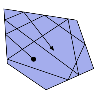
Figure 1: Left: In the weight space of a perceptron, the version space is a polytope. Ruján (1997) suggests playing billiards in weight space: averaging the ergodic trajectory of a reflected billiard ball to approximate the Bayes classifier. Right: In the function space of an NN binary classifier, where the axes measure the training outputs, the version space is an orthant. This paper suggests playing baseball in function space: maximising the normalised margin on the training data to approximate the Bayes classifier.

Consider an $L$-layer multi-layer perceptron $f_{L}:\mathcal{X}\times\mathcal{W}\to\mathbb{R}$ with weight matrices $w=(W_{1},...,W_{L})\in\mathcal{W}$ and nonlinearity set to $\mathrm{relu}(\cdot):=\max(0,\cdot)$:

$$f_{L}(x;w):=W_{L}\circ\mathrm{relu}\circ W_{L-1}\circ...\circ\mathrm{relu}\circ W_{1}(x).$$

A prior distribution $P_{\sigma}$ over weight space $\mathcal{W}$ is constructed by sampling each weight entry iid $\mathcal{N}(0,\sigma^{2})$. This induces a prior over functions with mean and covariance given by:

$$\mu_{\sigma}(x) :=\operatorname{\mathbb{E}}_{w\sim P_{\sigma}}[f_{L}(x;w)]=0;$$

$$k_{\sigma}(x,x^{\prime}) :=\operatorname{\mathbb{E}}_{w\sim P_{\sigma}}[f_{L}(x;w)f_{L}(x^{\prime};w)]=\sigma^{2L}k_{1}(x,x^{\prime}).$$

The first equality follows since $\operatorname{\mathbb{E}}_{w\sim P}{W_{L}}=0$. The second is due to the degree-$L$ positive homogeneity of the $\mathrm{relu}$ MLP. It follows that, for $n$ training inputs $X=\{x_{1},...,x_{n}\}$ and a test input $x$, the Gram matrix, vector and scalar satisfy:

$$K_{XX}=\sigma^{2L}\widehat{K}_{XX};\;K_{xX}=\sigma^{2L}\widehat{K}_{xX};\;K_{xx}=\sigma^{2L}\widehat{K}_{xx},$$

where $K$ and $\widehat{K}$ correspond to $k_{\sigma}$ and $k_{1}$, respectively.

By the NN–GP correspondence (Neal, 1994; Lee et al., 2018; de G. Matthews et al., 2018), as the MLP width is sent to infinity, the prior over functions converges to a GP with covariance $k_{\sigma}(x,x^{\prime})$. Consider using this GP to classify a test point $x$ by regressing to training inputs $X$ and binary labels $Y$. One is free to first scale up the labels by a margin parameter $\gamma>0$—see Figure 1. Conditioned on interpolating $(X,\gamma Y)$, a posterior prediction is given by:

$$\operatorname{sign}\left(K_{xX}K_{XX}^{-1}(\gamma Y)+\eta\cdot\sqrt{K_{xx}-K_{xX}K_{XX}^{-1}K_{Xx}}\right)$$

$$=\operatorname{sign}\left(\widehat{K}_{xX}\widehat{K}_{XX}^{-1}Y+\frac{\sigma^{L}}{\gamma}\cdot\eta\cdot\sqrt{\widehat{K}_{xx}-\widehat{K}_{xX}\widehat{K}_{XX}^{-1}\widehat{K}_{Xx}}\right),$$

for $\eta\sim\mathcal{N}(0,1)$. So by taking the normalised margin $\gamma/\sigma^{L}\to\infty$, an NN–GP’s entire function space in effect concentrates on the kernel interpolator $\widehat{K}_{xX}\widehat{K}_{XX}^{-1}Y$, which is itself a Bayes point machine by the results of Section 4.1.

5 Kernel PAC-Bayes

This section combines the results from Sections 3 and 4 with a novel bound on Gaussian orthant probabilities in order to derive risk bounds for kernel interpolators—and also for infinite width NNs by the results of Section 4.2.

The starting point is a well-known bound on the Gibbs error, that follows from Theorem 3 of Langford & Seeger (2001):

Lemma 7 (Gibbs PAC-Bayes).

Let $P$ be a prior over functions realised by a classifier. With probability $1-\delta$ over the $n$ iid training examples drawn from $\mathcal{D}$, for any posterior $Q$ over functions that correctly classify the training data:

$$\varepsilon_{\mathrm{Gibbs}}\leq 1-\exp\left(-\frac{\mathrm{KL}(Q||P)+\log(2n/\delta)}{n-1}\right).$$

To apply this lemma to a GP classifier, an appropriate KL divergence is needed. A draw from the GP prior correctly classifies the training data when the sampled labels $\Upsilon$ on the training inputs have the correct sign: $\operatorname{sign}\Upsilon=Y$. Thus, for the purposes of Lemma 7, it is enough to only consider distributions over the training labels. The prior, posterior and approximate posterior are then given by:

$$P_{\mathrm{GP}}:\qquad \Upsilon\sim\mathcal{N}\big{(}0,K_{XX}\big{)};\hskip 31.49998pt$$

$$Q_{\mathrm{GP}}:\qquad \Upsilon\sim\mathcal{N}\big{(}0,K_{XX}|\operatorname{sign}\Upsilon=Y\big{)};$$

$$Q_{\mathrm{iso}}:\qquad \Upsilon\sim\mathcal{N}\big{(}0,\mathbb{I}\cdot|{K_{XX}}|^{1/n}|\operatorname{sign}\Upsilon=Y\big{)}.$$

To derive the corresponding KL divergences, it is first useful to define the Gaussian orthant probability $P_{Y}$ of the orthant picked out by the binary vector $Y\in\{\pm 1\}^{n}$ via:

$$P_{Y}:=\mathbb{P}_{\Upsilon\sim P_{\mathrm{GP}}}[\operatorname{sign}\Upsilon=Y].$$

It is also useful to define another kernel complexity measure:

$$\mathcal{A}(k,X,Y):=n\cdot(\log 2-\tfrac{1}{2})\;+\qquad\qquad\qquad\qquad$$

$$|{K_{XX}}|^{1/n}\cdot\left[(\tfrac{1}{2}-\tfrac{1}{\pi})\operatorname{tr}K_{XX}^{-1}+\tfrac{1}{\pi}Y^{T}K_{XX}^{-1}Y\right].$$

This paper then obtains the following exact KL divergences:

Proof.

To establish the first equality, observe that:

$$\mathrm{KL}(Q_{\mathrm{GP}}||P_{\mathrm{GP}})=\operatorname{\mathbb{E}}_{\Upsilon\sim Q_{\mathrm{GP}}}\log(1/P_{Y})=\log(1/P_{Y}).$$

The last equality is derived by first observing that:

$$\mathrm{KL}(Q_{\mathrm{iso}}||P_{\mathrm{GP}})=\operatorname{\mathbb{E}}_{\Upsilon\sim Q_{\mathrm{iso}}}\log\frac{2^{n}\cdot\mathrm{e}^{-\tfrac{1}{2}\Upsilon^{2}|{K_{XX}}|^{-1/n}}}{\mathrm{e}^{-\tfrac{1}{2}\Upsilon^{T}K_{XX}^{-1}\Upsilon}}\qquad$$

$$=n\log 2+\tfrac{1}{2}\operatorname{\mathbb{E}}_{\Upsilon\sim\mathbb{Q}_{\mathrm{iso}}}[\Upsilon^{T}(K_{XX}^{-1}-\mathbb{I}|{K_{XX}}|^{-1/n})\Upsilon].$$

To complete the result, one must substitute in the identity:

$$\operatorname{\mathbb{E}}_{\Upsilon\sim\mathbb{Q}_{\mathrm{iso}}}[\Upsilon_{i}\Upsilon_{j}]=|{K_{XX}}|^{1/n}\cdot\left[\delta_{ij}+\tfrac{2}{\pi}Y_{i}Y_{j}(1-\delta_{ij})\right].$$

Finally, the inequality follows via:

$$\mathrm{KL}(Q_{\mathrm{iso}}||P_{\mathrm{GP}}) =\operatorname{\mathbb{E}}_{\Upsilon\sim Q_{\mathrm{iso}}}\left[\log\tfrac{Q_{\mathrm{iso}}(\Upsilon)}{Q_{\mathrm{GP}}(\Upsilon)}+\log\tfrac{Q_{\mathrm{GP}}(\Upsilon)}{P_{\mathrm{GP}}(\Upsilon)}\right]$$

$$=\mathrm{KL}(Q_{\mathrm{iso}}||Q_{\mathrm{GP}})+\log(1/P_{Y}),$$

and noting that $\mathrm{KL}(Q_{\mathrm{iso}}||Q_{\mathrm{GP}})\geq 0$. ∎

By combining Lemmas 3, 7 and 8 with the observation in Section 4.1 that kernel interpolators are BPMs corresponding to linear classifiers with log-concave posteriors supported on a convex set, the following result is immediate:

Four important remarks are in order:

First, the complexity term $\log(1/P_{Y})$ measures the degree of surprise experienced upon observing data sample $(X,Y)$ after fixing kernel $k(\cdot,\cdot)$. The smaller the surprise, the smaller the risk bound on $f_{Y_{\leavevmode\hbox to2.4pt{\vbox to2.4pt{\text{[drawing]}}}}}(x)$. The bound is non-vacuous when the sample is sufficiently unsurprising.

Second, $\mathcal{A}(k,X,Y)\geq\log(1/P_{Y})$ by Lemma 8, so the centre-of-mass interpolator $f_{Y_{\leavevmode\hbox to2.4pt{\vbox to2.4pt{\text{[drawing]}}}}}(x)$ enjoys a smaller risk bound than the centroidal interpolator $f_{Y}(x)$. If $f_{Y_{\leavevmode\hbox to2.4pt{\vbox to2.4pt{\text{[drawing]}}}}}(x)$ can be computed, it may indeed outperform $f_{Y}(x)$.

Third, the bounds admit a functional analytic interpretation. The term $Y^{T}K_{XX}^{-1}Y=(K_{XX}^{-1}Y)^{T}K_{XX}(K_{XX}^{-1}Y)$ appearing in $\mathcal{A}(k,X,Y)$ is the squared RKHS-norm of $f_{Y}(x)$. Similarly, $\log(1/P_{Y})$ is a form of log-sum-exp aggregate of the squared RKHS-norm across the version space:

$$\log(1/P_{Y})=-\log\int\limits_{\mathclap{\operatorname{sign}\Upsilon=Y}}\exp(-\tfrac{1}{2}\|f_{\Upsilon}\|_{\mathcal{H}}^{2})\,\mathrm{d}{\Upsilon}+\tfrac{1}{2}\log(2\pi)^{n}|{K_{XX}}|.$$

Fourth, the theorem applies (with probability one) to infinitely wide NNs whose normalised margin is sent to infinity ($\gamma/\sigma^{L}\to\infty$) by the argument given in Section 4.2.

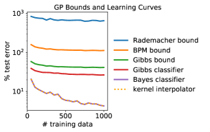
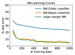
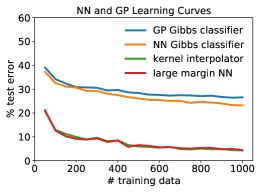
Figure 2: Left: Testing the theory for kernel interpolation. This plot serves two purposes: First, it compares the risk bounds in Theorem 1 and Lemma 7 to a classic Rademacher bound of Bartlett & Mendelson (2002). The Gibbs bound is non-vacuous, while the BPM bound is roughly an order-of-magnitude tighter than the Rademacher bound—although both are vacuous. Second, the plot displays near perfect agreement between the empirical isotropic Bayes classifier and the centroidal kernel interpolator, validating this paper’s central theme. Middle: Testing the theory for finite width multi-layer perceptrons (MLPs). This plot compares the test error of an ensemble of 501 small-margin MLPs—each trained to interpolate labels sampled from the label orthant—to a single large-margin MLP. The large-margin MLP closely matches the Bayes classifier. Right: Overlaying the kernel and finite width NN results. This plot displays close agreement between a single large-margin MLP and a kernel interpolator that uses the neural network–Gaussian process (NN–GP) equivalent kernel. Overall, these results suggest that finite width NNs trained to large margin may indeed approximate their own Bayes classifier.

6 Experiments

The purpose of this section is both to test the developed theory and to assess how well it may transfer to finite width NNs. An extensive investigation involving varied datasets and network architectures was beyond this paper’s wherewithal and is left to future work. But the authors believe that the results in Figure 2 are already quite interesting.

The experimental setup involved even/odd classification of MNIST handwritten digits (LeCun et al., 1998). The GP and kernel experiments used the compositional arccosine kernel (Cho & Saul, 2009; Daniely et al., 2016; Lee et al., 2018) which is the NN–GP equivalent kernel of an $L$-layer $\mathrm{relu}$ MLP. For two inputs $x,x^{\prime}\in\mathbb{R}^{d_{0}}$, it is given by:

$$k(x,x^{\prime}):=\underbrace{h\circ...\circ h}_{L-1\text{ times}}\left(\frac{x^{T}x^{\prime}}{d_{0}}\right),$$

where $h(t):=\tfrac{1}{\pi}\cdot[\sqrt{1-t^{2}}+t\cdot(\pi-\arccos t)].$ Inputs were normalised to $\|x\|_{2}^{2}=d_{0}$ so that $k(x,x)=1$.

The experiments resorted to the centroidal kernel interpolator since—despite having better theoretical properties—the centre-of-mass kernel interpolator seems intractable to compute. Correspondingly, the GP experiments used the isotropic Gibbs and Bayes classifiers—see Section 4.1.

The finite width NN experiments used width-1000, depth-7 $\mathrm{relu}$ MLPs trained using the Nero optimiser (Liu et al., 2021). Small margin NNs were each trained to fit a label vector drawn $\Upsilon\sim Q_{\mathrm{iso}}$ by minimising the loss:

$$\mathcal{L}_{\Upsilon}(w):=\sqrt{\frac{1}{n}\sum_{i}(f(x_{i},w)-\Upsilon_{i})^{2}}.$$

The large margin NN was trained to minimise $\mathcal{L}_{100\cdot Y}$.

6.1 Comparing Bounds

First the PAC-Bayes bounds of Theorem 1 and Lemma 7 were compared to a Rademacher bound (Bartlett & Mendelson, 2002, Theorem 21), which in this paper’s setting says that the risk of the centroidal kernel interpolator obeys:

$$\varepsilon_{Y}\leq 4\cdot\sqrt{Y^{T}K_{XX}^{-1}Y/n}+\mathrm{confidence\,term}.$$

This paper neglected the confidence term, so the Rademacher curve in Figure 2 (left) is a slight underestimate. Nevertheless, the Rademacher bound was nearly an order-of-magnitude worse than the BPM bound, which was itself a factor $\mathrm{e}$ worse than the non-vacuous Gibbs bound.

6.2 Quality of the BPM Approximation

To what extent does a Bayes point machine really reflect the majority behaviour of an entire ensemble? For NN–GPs, this question was studied by comparing the test error of the centroidal kernel interpolator to both the Gibbs and Bayes error of an ensemble of $10^{5}$ GP posterior draws. As can be seen in Figure 2 (left) the kernel interpolator almost perfectly recovered the error of the Bayes classifier, and both substantially outperformed the Gibbs classifier.

For finite width NNs, the Gibbs and Bayes classifiers were approximated by training an ensemble of 501 small margin NNs. These were then compared to the performance of a single large margin NN. As can be seen in Figure 2 (middle), the performance of the large margin NN closely matched the test performance of the approximate Bayes classifier, and both outperformed the approximate Gibbs classifier.

Finally, the NN-GP and finite width NN results are overlayed in Figure 2 (right).

7 Discussion and Future Work

This section highlights connections to existing research tracks, and the potential for exciting future work, by extracting three concrete suggestions from the developed theory.

Suggestion #1: Interpolate the Centre-of-Mass

Prior work comments on how arbitrary it is to classify by interpolating binary labels $Y$, since any labelling $\Upsilon$ in the orthant $\operatorname{sign}\Upsilon=Y$ yields correct training predictions (Liang & Recht, 2021). The theory in this paper suggests that interpolating centre-of-mass labels $Y_{\leavevmode\hbox to3.2pt{\vbox to3.2pt{\text{[drawing]}}}}:=\operatorname{\mathbb{E}}_{\Upsilon\sim Q_{\mathrm{GP}}}\Upsilon$ is more principled for two reasons: First, Section 4.1 show that it more directly approximates the GP Bayes classifier. Second, Theorem 1 shows that it enjoys a smaller risk bound.

Conceptually, the centre-of-mass kernel interpolator involves using the kernel’s prior to re-label the data before fitting. This bears a striking resemblance to the idea of self-distillation (Furlanello et al., 2018), which trains a teacher NN on the training data, and then retrains a student NN on the teacher’s predictions. Self-distillation and related techniques such as label smoothing (Müller et al., 2019) and label mixup (Zhang et al., 2018) have been found to improve generalisation performance in practice.

Studying self-distillation as an approximate centre-of-mass BPM could potentially unify and extend prior studies on self-distillation that use both Bayes theory (Zhang & Sabuncu, 2020) and functional analysis (Mobahi et al., 2020).

Suggestion #2: Maximise the Normalised Margin

While this suggestion is perhaps unsurprising, the authors feel it may have value in putting standard NN techniques on a more solid footing. Section 4.2 showed that to convert an infinite width NN into a BPM, one must select an interpolator which maximises a quantity $\gamma/\sigma^{L}$. The margin $\gamma$ measures the size of the training predictions, and the quantity $\sigma$ measures the scale of the weights at each layer. In NN classification, this motivates one of two strategies:

1. Use a margin maximizing loss (Rosset et al., 2003) such as cross-entropy and fix the weight norms;

2. Pair a loss function that targets a fixed margin such as mean squared error with $\ell_{2}$ regularisation.

Of course, both strategies are in use (Hui & Belkin, 2021). This theoretical suggestion ties in closely with prior work on the implicit bias of optimisation procedures (Barrett & Dherin, 2021; Smith et al., 2021) in their ability to target large margin functions (Soudry et al., 2018).

Suggestion #3: The Evidence is not Enough

Prior work on Bayesian model selection suggests choosing a GP kernel (van der Wilk et al., 2018) or NN architecture (Valle-Pérez & Louis, 2020; Immer et al., 2021) by maximising the marginal likelihood of the data under the model, also known as the evidence for the model (MacKay, 2003). Due to the difficultly of directly computing the evidence for a high-dimensional model, an evidence lower bound (ELBO) is often maximised as proxy (Wu et al., 2019).

The evidence for a GP binary classifier is nothing but the prior probability of the version space $\operatorname{sign}\Upsilon=Y$. This is denoted by the Gaussian orthant probability $P_{Y}$ in Section 5. This evidence $P_{Y}$ and its lower bound $\exp-\mathcal{A}(k,X,Y)$ take centre stage in Theorem 1, where they are used to upper bound the risk of kernel interpolation.

But looking at the empirical results in Figure 2 (left), both the BPM bound and the Gibbs bound are very loose in comparison to the actual performance of both the Bayes classifier and the kernel interpolator. In other words: ELBO maximisation—and also approximate evidence maximisation (Valle-Pérez & Louis, 2020)—is optimising a loose bound on the risk of the most desirable single classifier: the Bayes point machine. This is Seeger (2003)’s “dilemma”.

A jumping-off point for future work is to explore kernel and NN architecture design by optimising a more optimistic bound on the Bayes error such as Lemma 5—or more recent alternatives (Masegosa et al., 2020). The essential implication of Lemma 5 is that not only should the Gibbs error $\varepsilon_{\mathrm{Gibbs}}$ be minimised, but the version space should also include a sufficient diversity of opinion so as to make the Gibbs agreement $\alpha_{\mathrm{Gibbs}}$ small. This language is deliberately evocative of concepts in voter aggregation and social choice (Arrow, 1951; Kramer, 1977; Caplin & Nalebuff, 1988, 1991), since it is hoped that more of that literature may be brought to bear upon the learning problem.

8 Conclusion

This paper has developed a novel synthesis of ideas and techniques to characterise generalisation in interpolating learning machines. This synthesis draws on the literatures of statistical machine learning, social choice theory and convex geometry. The paper adds to a growing body of work that exploits hidden convexity to explain perplexing phenomena in neural networks (Jacot et al., 2018). In this paper, it is the convexity of version space when lifted to function space, and the log-concavity of the associated posterior.

At the heart of the paper is an old idea (Watkin, 1993; Ruján, 1997) that learners can attempt to point-approximate their own majority classifier. The paper shows how this idea—the Bayes point machine (Herbrich et al., 2001)—may be extended to multi-layer NNs, and how it may be used to derive simple risk bounds for interpolating classifiers. The paper opens up many exciting directions for future work. The authors are curious of where these directions may lead.

References

- Ambroladze et al. (2007) Ambroladze, A., Parrado-Hernández, E., and Shawe-Taylor, J. Tighter PAC-Bayes bounds. In Neural Information Processing Systems, 2007.
- Arrow (1951) Arrow, K. J. Social Choice and Individual Values. Wiley, 1951.
- Barrett & Dherin (2021) Barrett, D. and Dherin, B. Implicit gradient regularization. In International Conference on Learning Representations, 2021.
- Bartlett & Mendelson (2002) Bartlett, P. L. and Mendelson, S. Rademacher and Gaussian complexities: Risk bounds and structural results. Journal of Machine Learning Research, 2002.
- Bartlett et al. (2020) Bartlett, P. L., Long, P. M., Lugosi, G., and Tsigler, A. Benign overfitting in linear regression. Proceedings of the National Academy of Sciences, 2020.
- Belkin et al. (2018) Belkin, M., Ma, S., and Mandal, S. To understand deep learning we need to understand kernel learning. In International Conference on Machine Learning, 2018.
- Biggs & Guedj (2021) Biggs, F. and Guedj, B. On margins and derandomisation in PAC-Bayes. arXiv:2107.03955, 2021.
- Bordelon et al. (2020) Bordelon, B., Canatar, A., and Pehlevan, C. Spectrum dependent learning curves in kernel regression and wide neural networks. In International Conference on Machine Learning, 2020.
- Breiman (1996) Breiman, L. Bagging predictors. Machine Learning, 1996.
- Bubeck & Sellke (2021) Bubeck, S. and Sellke, M. A universal law of robustness via isoperimetry. In Neural Information Processing Systems, 2021.
- Caplin & Nalebuff (1988) Caplin, A. and Nalebuff, B. On 64%-majority rule. Econometrica, 1988.
- Caplin & Nalebuff (1991) Caplin, A. and Nalebuff, B. Aggregation and social choice: A mean voter theorem. Econometrica, 1991.
- Chatterji & Long (2020) Chatterji, N. S. and Long, P. M. Finite-sample analysis of interpolating linear classifiers in the overparameterized regime. Journal of Machine Learning Research, 2020.
- Cho & Saul (2009) Cho, Y. and Saul, L. Kernel methods for deep learning. In Neural Information Processing Systems, 2009.
- Condorcet (1785) Condorcet, N. d. Essai sur l’Application de l’Analyse à la Probabilité des Décisions Rendues à la Pluralité des Voix. Imprimerie Royale, 1785.
- Daniely et al. (2016) Daniely, A., Frostig, R., and Singer, Y. Toward deeper understanding of neural networks: The power of initialization and a dual view on expressivity. In Neural Information Processing Systems, 2016.
- de G. Matthews et al. (2018) de G. Matthews, A. G., Hron, J., Rowland, M., Turner, R. E., and Ghahramani, Z. Gaussian process behaviour in wide deep neural networks. In International Conference on Learning Representations, 2018.
- Devroye et al. (1996) Devroye, L., Györfi, L., and Lugosi, G. A probabilistic theory of pattern recognition. In Stochastic Modelling and Applied Probability, 1996.
- Dziugaite & Roy (2017) Dziugaite, G. K. and Roy, D. M. Computing nonvacuous generalization bounds for deep (stochastic) neural networks with many more parameters than training data. In Uncertainty in Artificial Intelligence, 2017.
- Freund & Schapire (1996) Freund, Y. and Schapire, R. E. Experiments with a new boosting algorithm. In International Conference on Machine Learning, 1996.
- Furlanello et al. (2018) Furlanello, T., Lipton, Z. C., Tschannen, M., Itti, L., and Anandkumar, A. Born again neural networks. In International Conference on Machine Learning, 2018.
- Germain et al. (2015) Germain, P., Lacasse, A., Laviolette, F., Marchand, M., and Roy, J.-F. Risk bounds for the majority vote: From a PAC-Bayesian analysis to a learning algorithm. Journal of Machine Learning Research, 2015.
- Girosi et al. (1995) Girosi, F., Jones, M., and Poggio, T. Regularization theory and neural networks architectures. Neural Computation, 1995.
- Grünbaum (1960) Grünbaum, B. Partitions of mass-distributions and of convex bodies by hyperplanes. Pacific Journal of Mathematics, 1960.
- Herbrich (2001) Herbrich, R. Learning Kernel Classifiers: Theory and Algorithms. MIT Press, 2001.
- Herbrich et al. (2001) Herbrich, R., Graepel, T., and Campbell, C. Bayes point machines. Journal of Machine Learning Research, 2001.
- Hui & Belkin (2021) Hui, L. and Belkin, M. Evaluation of neural architectures trained with square loss vs. cross-entropy in classification tasks. In International Conference on Learning Representations, 2021.
- Immer et al. (2021) Immer, A., Bauer, M., Fortuin, V., Rätsch, G., and Emtiyaz, K. M. Scalable marginal likelihood estimation for model selection in deep learning. In International Conference on Machine Learning, 2021.
- Jacot et al. (2018) Jacot, A., Gabriel, F., and Hongler, C. Neural tangent kernel: Convergence and generalization in neural networks. In Neural Information Processing Systems, 2018.
- Kanagawa et al. (2018) Kanagawa, M., Hennig, P., Sejdinovic, D., and Sriperumbudur, B. K. Gaussian processes and kernel methods: A review on connections and equivalences. arXiv:1807.02582, 2018.
- Kramer (1977) Kramer, G. H. A dynamical model of political equilibrium. Journal of Economic Theory, 1977.
- Lacasse et al. (2007) Lacasse, A., Laviolette, F., Marchand, M., Germain, P., and Usunier, N. PAC-Bayes bounds for the risk of the majority vote and the variance of the Gibbs classifier. In Neural Information Processing Systems, 2007.
- Langford & Seeger (2001) Langford, J. and Seeger, M. Bounds for averaging classifiers. Technical report, Carnegie Mellon University, 2001.
- Langford & Shawe-Taylor (2003) Langford, J. and Shawe-Taylor, J. PAC-Bayes & margins. In Neural Information Processing Systems, 2003.
- LeCun et al. (1998) LeCun, Y., Cortes, C., and Burges, C. J. MNIST handwritten digit database, 1998.
- Lee et al. (2018) Lee, J., Sohl-Dickstein, J., Pennington, J., Novak, R., Schoenholz, S., and Bahri, Y. Deep neural networks as Gaussian processes. In International Conference on Learning Representations, 2018.
- Liang & Rakhlin (2020) Liang, T. and Rakhlin, A. Just interpolate: Kernel “ridgeless” regression can generalize. The Annals of Statistics, 2020.
- Liang & Recht (2021) Liang, T. and Recht, B. Interpolating classifiers make few mistakes. arXiv:2101.11815, 2021.
- Liu et al. (2021) Liu, Y., Bernstein, J., Meister, M., and Yue, Y. Learning by turning: Neural architecture aware optimisation. In International Conference on Machine Learning, 2021.
- MacKay (2003) MacKay, D. J. C. Information Theory, Inference, and Learning Algorithms. Cambridge University Press, 2003.
- Masegosa et al. (2020) Masegosa, A. R., Lorenzen, S. S., Igel, C., and Seldin, Y. Second order PAC-Bayesian bounds for the weighted majority vote. In Neural Information Processing Systems, 2020.
- McAllester (1998) McAllester, D. A. Some PAC-Bayesian theorems. In Conference on Computational Learning Theory, 1998.
- Meir & Zhang (2003) Meir, R. and Zhang, T. Generalization error bounds for Bayesian mixture algorithms. Journal of Machine Learning Research, 2003.
- Mobahi et al. (2020) Mobahi, H., Farajtabar, M., and Bartlett, P. L. Self-distillation amplifies regularization in Hilbert space. In Neural Information Processing Systems, 2020.
- Müller et al. (2019) Müller, R., Kornblith, S., and Hinton, G. When does label smoothing help? In Neural Information Processing Systems, 2019.
- Nakkiran et al. (2020) Nakkiran, P., Kaplun, G., Bansal, Y., Yang, T., Barak, B., and Sutskever, I. Deep double descent: Where bigger models and more data hurt. In International Conference on Learning Representations, 2020.
- Neal (1994) Neal, R. M. Bayesian Learning for Neural Networks. Ph.D. thesis, Department of Computer Science, University of Toronto, 1994.
- Neyshabur et al. (2018) Neyshabur, B., Bhojanapalli, S., and Srebro, N. A PAC-Bayesian approach to spectrally-normalized margin bounds for neural networks. In International Conference on Learning Representations, 2018.
- Opper (2001) Opper, M. Learning to generalize. Frontiers of Life, 2001.
- Rivasplata et al. (2020) Rivasplata, O., Kuzborskij, I., Szepesvári, C., and Shawe-Taylor, J. PAC-Bayes analysis beyond the usual bounds. In Neural Information Processing Systems, 2020.
- Rosset et al. (2003) Rosset, S., Zhu, J., and Hastie, T. Margin maximizing loss functions. In Neural Information Processing Systems, 2003.
- Ruján (1997) Ruján, P. Playing billiards in version space. Neural Computation, 1997.
- Ruján & Marchand (2000) Ruján, P. and Marchand, M. Computing the Bayes kernel classifier. In Advances in Large-Margin Classifiers, 2000.
- Seeger (2003) Seeger, M. PAC-Bayesian generalisation error bounds for Gaussian process classification. Journal of Machine Learning Research, 2003.
- Shawe-Taylor & Williamson (1997) Shawe-Taylor, J. and Williamson, R. C. A PAC analysis of a Bayesian estimator. In Conference on Learning Theory, 1997.
- Simpson (1969) Simpson, P. B. On defining areas of voter choice: Professor Tullock on stable voting. The Quarterly Journal of Economics, 1969.
- Smith et al. (2021) Smith, S. L., Dherin, B., Barrett, D., and De, S. On the origin of implicit regularization in stochastic gradient descent. In International Conference on Learning Representations, 2021.
- Soudry et al. (2018) Soudry, D., Hoffer, E., Nacson, M. S., Gunasekar, S., and Srebro, N. The implicit bias of gradient descent on separable data. Journal of Machine Learning Research, 2018.
- Tukey (1977) Tukey, J. W. Exploratory Data Analysis. Addison-Wesley, 1977.
- Valle-Pérez & Louis (2020) Valle-Pérez, G. and Louis, A. A. Generalization bounds for deep learning. arXiv:2012.04115, 2020.
- van der Wilk et al. (2018) van der Wilk, M., Bauer, M., John, S., and Hensman, J. Learning invariances using the marginal likelihood. In Neural Information Processing Systems, 2018.
- Viallard et al. (2021) Viallard, P., Germain, P., Habrard, A., and Morvant, E. A general framework for the disintegration of PAC-Bayesian bounds. arXiv:2102.08649, 2021.
- Watkin (1993) Watkin, T. Optimal learning with a neural network. Europhysics Letters, 1993.
- Wu et al. (2019) Wu, A., Nowozin, S., Meeds, E., Turner, R. E., Hernandez-Lobato, J. M., and Gaunt, A. L. Deterministic variational inference for robust Bayesian neural networks. In International Conference on Learning Representations, 2019.
- Zhang et al. (2018) Zhang, H., Cisse, M., Dauphin, Y. N., and Lopez-Paz, D. mixup: Beyond empirical risk minimization. In International Conference on Learning Representations, 2018.
- Zhang & Sabuncu (2020) Zhang, Z. and Sabuncu, M. R. Self-distillation as instance-specific label smoothing. In Neural Information Processing Systems, 2020.