The Multiplicative Persistence Conjecture Is True for Odd Targets

Abstract

In 1973, Neil Sloane published a very short paper introducing an intriguing problem: Pick a decimal integer $n$ and multiply all its digits by each other. Repeat the process until a single digit $\Delta(n)$ is obtained. $\Delta(n)$ is called the multiplicative digital root of $n$ or the target of $n$. The number of steps $\Xi(n)$ needed to reach $\Delta(n)$, called the multiplicative persistence of $n$ or the height of $n$ is conjectured to always be at most $11$.

Like many other very simple to state number-theoretic conjectures, the multiplicative persistence mystery resisted numerous explanation attempts.

This paper proves that the conjecture holds for all odd target values:

• If $\Delta(n)\in\{1,3,7,9\}$, then $\Xi(n)\leq 1$

• If $\Delta(n)=5$, then $\Xi(n)\leq 5$

Naturally, we overview the difficulties currently preventing us from extending the approach to (nonzero) even targets.

1 Introduction

In 1973, Neil Sloane published a very short paper [Slo73] introducing an intriguing problem: Pick a decimal integer $n$ and multiply all its digits by each other. Repeat the process until a single digit $\Delta(n)$ is obtained. $\Delta(n)$ is called the multiplicative digital root of $n$ or the target of $n$. The number of steps $\Xi(n)$ needed to reach $\Delta(n)$, called the multiplicative persistence of $n$ or the height of $n$ is conjectured to always be at most $11$.

For instance, the target of $39$ is $4$, because:

$$39\rightarrow 3\times 9=27\rightarrow 2\times 7=14\rightarrow 1\times 4=4=\Delta(39)$$

Like many other very simple to state number-theoretic conjectures, the multiplicative persistence mystery resisted numerous explanation attempts [Wor80], [Sch], [PS], [McE19], [Dia11], [dFT14].

In particular, the conjecture is known to hold at least up to $n=10^{20000}$ [Wei].

Addressing the Multiplicative persistence conjectures consists in studying the function $f:n\rightarrow f(n)$, where $f(n)$ is obtained by multiplying the digits of the the number $n$.

$\Xi(n)$ is hence the smallest $k$ such that $f^{k}(n)\leq 9$.

Note that $\Xi(n)$ is defined for all $n\in\mathbb{N}$: letting $n=\sum_{i=0}^{r}10^{i}a_{i}$ (where the $0\leq a_{i}\leq 9$ are digits), $f(n)=\prod_{i=0}^{r}a_{i}<a_{r}\times 10^{r}\leq n$.

$\mathcal{F}_{n}=\{f(n),f^{2}(n),f^{3}(n),\ldots\}$ is thus a positive decreasing sequence, and as such, it converges.

Since $\mathcal{F}_{n}$ takes values in $\mathbb{N}$, $\mathcal{F}_{n}$ can only converge by reaching a fix-point $\Delta(n)$ and staying at it. However, the $\mathcal{F}_{n}$ is strictly decreasing while its values have at least two decimal digits.

Finally, $\mathcal{F}_{n}$ converges converges toward a one-digit number, $\Delta(n)\leq 9$. Hence the notion of multiplicative persistence $\Xi(n)$ defined as the number of steps required to reach $\Delta(n)$.

The following is a famous conjecture [K.81]:

Conjecture 1

$\forall n\in\mathbb{N}$, $\Xi(n)\leq 11$.

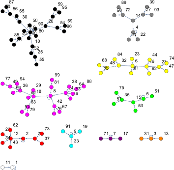
Figure 1: Genealogy for $0\leq n\leq 99$.

In this work we prove the conjecture for all odd targets and provide bounds for $\Xi(n)$ depending on the value of $\Delta(n)$.

1.1 Notations

To present formulae concisely, we introduce the following compact notation:

$$[\begin{smallmatrix}a&b\\ c&d\end{smallmatrix}]=2^{a}\times 3^{b}\times 5^{c}\times 7^{d}$$

When an exponent is zero we might just omit the corresponding entry in the notation, or replace it by a $0$ e.g.:

$$[\begin{smallmatrix}0&b\\ c&d\end{smallmatrix}]=[\begin{smallmatrix}&b\\ c&d\end{smallmatrix}]=3^{b}\times 5^{c}\times 7^{d}$$

$\mbox{{ord}}_{n}(a)$ will denote the order of $a\bmod n$, i.e. the smallest positive integer $k$ such that $a^{k}\ \equiv\ 1\bmod n$.

In this paper, the term “digit” will exclusively refer to decimal digits.

Let $d$ be a digit, the shorthand notation $d_{x}$ will stand for a sequence of $x$ consecutive digits $d$, e.g.:

$$9_{8}0_{7}1=9999999900000001$$

To simplify notations we will denote by $\vec{x}$ a sequence of $(k+1)$ indexed variables starting with $x_{0}$ and ending with $x_{k}$, that is: $\vec{x}=\mbox{``}x_{0},x_{1},\ldots,x_{k}\mbox{''}$. Operations on vectors are to be understood component wise, e.g.:

$$\vec{x}+7\vec{y}=\mbox{``}x_{0}+7y_{0},x_{1}+7y_{1},\ldots,x_{k}+7y_{k}\mbox{''}$$

Finally, we will also need the following definition:

Definition 1

$\mbox{{dec}}\llbracket\begin{smallmatrix}1&3&5&7&9\\ *&a&b&c&d\end{smallmatrix}\rrbracket$ denotes the set of decimal integers where the digits $3,5,7,9$ respectively appear $a,b,c,d$ times (at any position) with any number of $1$s.

The acronyms dnv, aad and anad will respectively stand for “do(es) not verify”, “are all different (from each other)” and “are not all different”. e.g. “$x=2$ dnv $x^{2}=5$”, “{1,2,3} aad”, “$a=1$, $b=2$ and $c=1$ anad.”

2 Convergence Genealogies

(P1) : Take $y$ an odd number. If $\exists x$ such that $f(x)=y$ then, as the product of the digits of $x$, $y$ can be written as $y=[\begin{smallmatrix}\alpha&\beta\\ \gamma&\delta\end{smallmatrix}]$. Since $y$ is odd, $y=[\begin{smallmatrix}&\beta\\ \gamma&\delta\end{smallmatrix}]$. As an antecedent of $y$, $x$ belongs to one of the sets $\mbox{{dec}}\llbracket\begin{smallmatrix}1&3&5&7&9\\ *&\beta_{1}&\gamma&\delta&\beta_{2}\end{smallmatrix}\rrbracket$, with $\beta_{1}+2\times\beta_{2}=\beta$. Conversely, if $y=[\begin{smallmatrix}&\beta\\ \gamma&\delta\end{smallmatrix}]$ and $x\in\mbox{{dec}}\llbracket\begin{smallmatrix}1&3&5&7&9\\ *&\beta_{1}&\gamma&\delta&\beta_{2}\end{smallmatrix}\rrbracket$, with $\beta_{1}+2\times\beta_{2}=\beta$, then $f(x)=y$.

Let us notice that if $\Delta(n)$ is odd, then $n$ has to be odd too: indeed, if $n$ would have been even, its last digit would be even as well, and thus $f(n)$ would be even, and so on.

For a digit $d$, let us denote as tree of antecedents of $d$ the graph $A_{d}=(V_{d},E_{d})$ defined as follows:

• $d\in V_{d}$

• If $s\in V_{d}$ and $x$ such that $f^{2}(x)=s$, then $f(x)\in V_{d}$ and $(s,f(x))\in E_{d}$

(P2) : Then, $\{n:\Delta(n)=d\}=\{n:f(n)\in V_{d}\}$, and $\Xi(n)$ for $n$ such that $\Delta(n)=d$ is the number of different nodes in the path connecting $d$ to $f(n)$.

(P1) and (P2) together with the knowledge of $A_{1}$, $A_{3}$, $A_{5}$, $A_{7}$ and $A_{9}$ describe all numbers $n$ such that $\Delta(n)=d$ for a given odd digit $d$. We now want to prove that $A_{1}$, $A_{3}$, $A_{5}$, $A_{7}$ and $A_{9}$ are respectively the following graphs:

$B_{1}=(U_{1},F_{1})$ =   

$B_{3}=(U_{3},F_{3})$ =   

$B_{5}=(U_{5},F_{5})$ =

$B_{7}=(U_{7},F_{7})$ =   

$B_{9}=(U_{9},F_{9})$ =   

3 Establishing the Equations

The five graphs above are respectively sub-graphs of $A_{1}$, $A_{3}$, $A_{5}$, $A_{7}$ and $A_{9}$. To prove that they are also equal to said graphs, we need to prove for $d\in\{1;\ 3;\ 5;\ 7;\ 9\}$ that for each $s\in U_{d}$, if $x$ is such that $f^{2}(x)=s$, then $f(x)\in U_{d}$.

For example take $d=1$ and $s=1$. Let us consider $x$ such that $f^{2}(x)=s$. Because $1=[\begin{smallmatrix}&0\\ 0&0\end{smallmatrix}]$, (P1) gives that $f(x)\in\mbox{{dec}}\llbracket\begin{smallmatrix}1&3&5&7&9\\ *&0&0&0&0\end{smallmatrix}\rrbracket$, meaning that $f(x)$ is only composed of $1$s. Therefore, there exists $a$ (corresponding to the number of digits of $f(x)$) such that $f(x)=\frac{10^{a}-1}{9}$. On the other hand, $f(x)=[\begin{smallmatrix}&\beta\\ \gamma&\delta\end{smallmatrix}]$, and $f(x)$ has neither $0$ nor $5$ as digits since $f^{2}(x)=1$, so we have $\gamma=0$. We thus want to solve $\frac{10^{a}-1}{9}=[\begin{smallmatrix}0&\beta\\ 0&\delta\end{smallmatrix}]$, or equivalently: $10^{a}-1=[\begin{smallmatrix}0&u\\ 0&w\end{smallmatrix}]$.

For another example, take $d=5$ and $s=315$. Let us consider $x$ such that $f^{2}(x)=s$. Because $315=[\begin{smallmatrix}&2\\ 1&1\end{smallmatrix}]$, (P1) gives that either $f(x)\in\mbox{{dec}}\llbracket\begin{smallmatrix}1&3&5&7&9\\ *&2&1&1&0\end{smallmatrix}\rrbracket$ or $f(x)\in\mbox{{dec}}\llbracket\begin{smallmatrix}1&3&5&7&9\\ *&0&1&1&1\end{smallmatrix}\rrbracket$. Therefore, either

• there exist $a$ (corresponding to the number of digits of $f(x)$), and $b,c,d,e$ (corresponding respectively to the positions of the digits $3$, $3$, $5$ and $7$ in $f(x)$) such that $f(x)=\frac{10^{a}-1}{9}+(3-1)\times 10^{b}+(3-1)\times 10^{c}+(5-1)\times 10^{d}+(7-1)\times 10^{e}$ (with $a>b,c,d,e\geq 0$ and $b,c,d,e$ all different because of what $a,b,c,d,e$ represent),

• or there exist $a$ and $b,c,d$ such that $f(x)=\frac{10^{a}-1}{9}+(5-1)\times 10^{b}+(7-1)\times 10^{c}+(9-1)\times 10^{d}$.

On the other hand, $f(x)=[\begin{smallmatrix}&\beta\\ \gamma&\delta\end{smallmatrix}]$. We thus want to solve

• $10^{a}+18\times 10^{b}+18\times 10^{c}+36\times 10^{d}+54\times 10^{e}-1=[\begin{smallmatrix}&u\\ v&w\end{smallmatrix}]$

• and $10^{a}+36\times 10^{b}+54\times 10^{c}+72\times 10^{d}-1=[\begin{smallmatrix}&u\\ v&w\end{smallmatrix}]$

3.1 About the Possible Values of $v=\gamma$, the Power of $5$

If $d\neq 5$ is an odd digit, if $s\in U_{d}$ and $x$ such that $f^{2}(x)=s$, $f(x)=[\begin{smallmatrix}&\beta\\ \gamma&\delta\end{smallmatrix}]$ with $\gamma=0$ since $f(x)$ would otherwise end with $0$ or $5$, which would make $f^{k}(x)=d$ for some $k$ impossible.

For $d=5$ however, if $s\in U_{5}$ and $x$ such that $f^{2}(x)=s$, we initially only know that $f(x)=[\begin{smallmatrix}&\beta\\ \gamma&\delta\end{smallmatrix}]$.

Let us look at the values $[\begin{smallmatrix}&\beta\\ \gamma&\delta\end{smallmatrix}]$ takes if $\gamma\geq 5$: odd multiples of $5^{5}$ have their values modulo $10^{5}$ in:

{3125,	9375,	15625,	21875,	28125,	34375,	40625,	46875,
53125,	59375,	65625,	71875,	78125,	84375,	90625,	96875}

Therefore, if $f(x)=[\begin{smallmatrix}&\beta\\ \gamma&\delta\end{smallmatrix}]$ with $\gamma\geq 5$, either $f(x)=9375$ in $\mathbb{Z}$ or $f(x)\bmod 10^{5}=59375=[\begin{smallmatrix}0&5\\ 1&2\end{smallmatrix}]$. However, $f(9375)=945\notin U_{5}$. Furthermore, if $f(x)\bmod 10^{5}=59375$, $f^{2}(x)$ is a multiple of $4725$, but $4725$ divides no element of $U_{5}$. From that, we know that $\gamma\leq 4$.

Similarly, odd multiples of $5^{4}$ have their values modulo $10^{4}$ in :

$$\{625,1875,3125,4375,5625,6875,8125,9375\}$$

Thus, if $\gamma=4$, $s=f^{2}(x)$ is a multiple of $f(9375)=945$. Since $59535$ is the only element of $U_{5}$ that $945$ divides, $s=59535$. Note that knowing $f(x)\bmod 10^{4}=9375$ gives us the positions of some digits $9,3,7,5$ in $f(x)$.

Likewise, if $\gamma=3$, $f(x)\bmod 10^{3}=375$ and $f(375)=105$ divides $s=f^{2}(x)$, so $s\in\{315,1575,59535,77175\}=[\begin{smallmatrix}0&2\\ 1&1\end{smallmatrix}]\times\{1,5,189,245\}$.

If $\gamma=2$, $f(75)=35$ divides $s$, so $s\in\{35,175,315,1575,1715,59535,77175\}$.

Furthermore, because of the values $3^{\beta}\times 7^{\delta}$ takes modulo $100$ (the tens digit is always even), $\gamma\geq 1$.

3.2 Listing all Equations

To summarise, let us take $d$ an odd digit, $s\in U_{d}$ and $x$ such that $f^{2}(x)=s$. Then $f(x)=[\begin{smallmatrix}&\beta\\ \gamma&\delta\end{smallmatrix}]$ with $\gamma=0$ if $d\neq 5$, and $\gamma$ taking at most four different values from $\{1,2,3,4\}$ depending on $s$ if $d=5$. Also $f(x)\in\mbox{{dec}}\llbracket\begin{smallmatrix}1&3&5&7&9\\ *&h_{1}&i&j&h_{2}\end{smallmatrix}\rrbracket$, with $h_{1}+2\times h_{2}=h$ if $s=[\begin{smallmatrix}&h\\ i&j\end{smallmatrix}]$.

For all $d,s$ we can range over all possible split $(h_{1},h_{2})$ and all possible $\gamma$ to establish a finite list of equations that $f(x)$ must satisfy. The number of equations for all possible $d$ are as follows:

value of $d$	1	3	5	7	9
number of equations	1	1	39	1	2

Notice that when $\gamma\neq 0$, the knowledge of $f(x)\bmod 10^{\gamma}$ gives the position of the $\gamma$ last digits of $f(x)$, and they are always such that we are able to divide both sides of the equation by $5^{\gamma}$.

As a consequence, all equations can be put in the form $\mbox{{LC}}(\vec{a})=[\begin{smallmatrix}0&u\\ 0&w\end{smallmatrix}]$ where $\mbox{{LC}}(\vec{a})$ is a linear combination of $10^{a_{0}}$, $10^{a_{1}}$, …, $10^{a_{k}}$. Precisely, they are defined by the formula:

$$2^{h}\times(10^{a_{0}}+18\sum_{i=1}^{k}c_{i}\times 10^{a_{i}})+\tau_{h}=[\begin{smallmatrix}0&u\\ 0&w\end{smallmatrix}]$$

where

$h=\gamma$	$0$	$1$	$2$	$3$	$4$
$\tau_{h}$	$-1$	$7$	$23$	$19$	$119$

and where the other parameters are given in Appendix 0.A.

The solutions that interest us must verify (R) : $a_{0}>a_{1},\ldots,a_{k}$ and $a_{1},\ldots,a_{k}$ aad and non-negative. The following section describes a resolution algorithm for solving this kind of equations. It outputs a finite list of solutions from which one can verify that the only ones satisfying (R) correspond to values $f(x)$ belonging to $U_{d}$.

4 Resolution Algorithm

4.1 The General Principle

We want to solve (E) : $\mbox{{LC}}(\vec{a})=[\begin{smallmatrix}0&u\\ 0&w\end{smallmatrix}]$ where $\mbox{{LC}}(\vec{a})$ is a linear combination of $10^{a_{0}}$, $10^{a_{1}}$, …, $10^{a_{k}}$, $a_{0}>a_{1},\ldots,a_{k}$ and $a_{1},\ldots,a_{k}$ aad.

For some $t>0$ and $y,z\leq t$, assume that we know for $(\vec{a},u,w)$ a solution of (E) the residues $(\vec{a^{\prime}})=(\vec{a})\bmod t$, $u^{\prime}=u\bmod\mbox{{ord}}_{[\begin{smallmatrix}y&0\\ z&0\end{smallmatrix}]}(3)$, and $w^{\prime}=w\bmod\mbox{{ord}}_{[\begin{smallmatrix}y&0\\ z&0\end{smallmatrix}]}(7)$.

Because $\mbox{{LC}}(\vec{a})$ is a linear combination of $10^{a_{0}},10^{a_{1}},\ldots,10^{a_{k}}$, the knowledge of $(\vec{a})\bmod t$ gives at most $2^{k+1}$ possible values for $\mbox{{LC}}(\vec{a})\bmod[\begin{smallmatrix}y&0\\ z&0\end{smallmatrix}]$. Indeed, since $a_{i}=a^{\prime}_{i}+q_{i}\times t$ with $0\leq a^{\prime}_{i}<t$, we have

$$10^{a_{i}}=10^{a^{\prime}_{i}}\times(10^{t})^{q_{i}}\equiv 10^{a^{\prime}_{i}}\times(0)^{q_{i}}\bmod{[\begin{smallmatrix}y&0\\ z&0\end{smallmatrix}]}.$$

Thus, for each $i$, $10^{a_{i}}\bmod[\begin{smallmatrix}y&0\\ z&0\end{smallmatrix}]$ can take only two values: either $10^{a^{\prime}_{i}}$ (in which case $a_{i}$ is known in $\mathbb{Z}$) or $0$.

Note that the knowledge of $u^{\prime}=u\bmod\mbox{{ord}}_{[\begin{smallmatrix}y&0\\ z&0\end{smallmatrix}]}(3)$ and $w^{\prime}=w\bmod\mbox{{ord}}_{[\begin{smallmatrix}y&0\\ z&0\end{smallmatrix}]}(7)$ gives us $[\begin{smallmatrix}0&u\\ 0&w\end{smallmatrix}]\bmod[\begin{smallmatrix}y&0\\ z&0\end{smallmatrix}]$.

Considering the equation (E) modulo $[\begin{smallmatrix}y&0\\ z&0\end{smallmatrix}]$, we are able, for each $(\vec{b})=(b_{0},\ldots,b_{k})\in\{0,1\}^{k+1}$, to compute $\textsf{LC}(\vec{a})\bmod[\begin{smallmatrix}y&0\\ z&0\end{smallmatrix}]=\sum_{i}b_{i}10^{a^{\prime}_{i}}\bmod[\begin{smallmatrix}y&0\\ z&0\end{smallmatrix}]$ and check whether it is equal to $3^{u^{\prime}}\times 7^{w^{\prime}}\bmod[\begin{smallmatrix}y&0\\ z&0\end{smallmatrix}]$.

We want $y$ and $z$ to be high enough such that the congruence modulo $[\begin{smallmatrix}y&0\\ z&0\end{smallmatrix}]$ is satisfied for only a few $(\vec{b})$. This set of complying solutions can then be further reduced. Indeed, for each surviving $(\vec{b})$ one can check whether the partial set of known $a_{i}$ ($a_{i}$ is known in $\mathbb{Z}$ for all $i$ such that $b_{i}=1$) also complies with requirement (R). The hope is that each tuple $(\vec{a^{\prime}},u^{\prime},w^{\prime})$ we may start from, either yields a uniquely determined ($b_{i}=1$ for all $i$) solution $f(x)$ belonging to $U_{d}$, or no solution at all.

4.2 Application

Let us e.g. chose $(t,y,z)=(12,9,6)$. $\mbox{{ord}}_{[\begin{smallmatrix}9&0\\ 6&0\end{smallmatrix}]}(3)=[\begin{smallmatrix}7&0\\ 5&0\end{smallmatrix}]$ and $\mbox{{ord}}_{[\begin{smallmatrix}9&0\\ 6&0\end{smallmatrix}]}(7)=[\begin{smallmatrix}6&0\\ 4&0\end{smallmatrix}]$.

Let us notice that $10^{12}-1=[\begin{smallmatrix}0&3\\ 0&1\end{smallmatrix}]\times 11\times 13\times 37\times 101\times 9901$. Denote $m_{12}:=\frac{10^{12}-1}{3^{3}\times 7}=11\times 13\times 37\times 101\times 9901$. $m_{12}$ has the two following interesting properties:

• $\mbox{{ord}}_{m_{12}}(10)=12$

• and $([\begin{smallmatrix}0&u^{\prime}\\ 0&w^{\prime}\end{smallmatrix}]\equiv 1\bmod{m_{12}})\iff\left\{\begin{array}[]{l}u^{\prime}\equiv 0\bmod{9900}\\ w^{\prime}\equiv 0\bmod{900}\end{array}\right.$.

Assume that $(\vec{a},u,w)$ is a solution of (E). Let us look at all $0\leq a^{\prime}_{1},a^{\prime}_{2},\ldots a^{\prime}_{k}<12$ such that $\mbox{{LC}}(\vec{a^{\prime}})\equiv 3^{u^{\prime}}\times 7^{w^{\prime}}\bmod{m_{12}}$ for some $0\leq u^{\prime}<9900$ and $0\leq w^{\prime}<900$. Thanks to the two properties of $m_{12}$ mentioned here above, we can thus reduce the possible values of $(\vec{a})\bmod 12$ and get matching values for $u\bmod 9900$ and $w\bmod 900$.

At this point we have a set of possible values for $(\vec{a})\bmod 12$, and for each of them we know the corresponding values of $u^{\prime}=u\bmod(11\times[\begin{smallmatrix}2&2\\ 2&\phantom{0}\end{smallmatrix}])$ and $w^{\prime}=w\bmod[\begin{smallmatrix}2&2\\ 2&\phantom{0}\end{smallmatrix}]$. Remember that our goal is to know $u$ and $w$ modulo $[\begin{smallmatrix}7&0\\ 5&0\end{smallmatrix}]$ and $[\begin{smallmatrix}6&0\\ 4&0\end{smallmatrix}]$ respectively. To improve our knowledge of $u$ and $w$ our strategy is to lift from equation (E) considered modulo $m_{12}$ to (E) considered modulo $m_{24}:=\frac{10^{24}-1}{3^{3}\times 7}=m_{12}\times 73\times 137\times 9_{4}0_{3}1$.

For each value $(\vec{a})$ can take modulo 12, we obtain $2^{k+1}$ different values for $(\vec{a})\bmod 24$. Consider $p=73$ a prime divisor of $m_{24}$ and observe that $\mbox{{ord}}_{73}(3)=[\begin{smallmatrix}2&1\\ 0&0\end{smallmatrix}]$ and $\mbox{{ord}}_{73}(7)=[\begin{smallmatrix}3&1\\ 0&0\end{smallmatrix}]$. Since $\mbox{{ord}}_{73}(7)=[\begin{smallmatrix}3&1\\ 0&0\end{smallmatrix}]$ we can improve our knowledge of $w$ from $w\bmod[\begin{smallmatrix}2&2\\ 2&\phantom{0}\end{smallmatrix}]$ to $w\bmod[\begin{smallmatrix}3&2\\ 2&\phantom{0}\end{smallmatrix}]$. This is due to the principle described in Section 4.3. Considering other prime divisors of $m_{24}$ progressively further improves our knowledge of $u$ and $w$. As this knowledge is not yet sufficient, we eventually have to lift upper from $m_{24}$ to $m_{48}:=\frac{10^{48}-1}{3^{3}\times 7}$ and exploit other prime divisors of $m_{48}$ up to obtaining our sufficient knowledge of $u\bmod[\begin{smallmatrix}7&0\\ 5&0\end{smallmatrix}]$ and $w\bmod[\begin{smallmatrix}6&0\\ 4&0\end{smallmatrix}]$.

4.3 Improving our knowledge of $u$ and $w$

Suppose that we know the value of $\mbox{{LC}}(\vec{a})\bmod p$. Suppose that we have $m_{u}$ and $m_{w}$ such that we know of $0\leq u^{\prime}<m_{u}$ and $0\leq w^{\prime}<m_{w}$ verifying $u=u^{\prime}+h_{u}m_{u}$ and $w=w^{\prime}+h_{w}m_{w}$. Suppose that $q$, $n_{u}=\lambda\times m_{u}$ and $n_{w}=\mu\times m_{w}$ are such that $\mbox{{ord}}_{p}(3)$ divides $q\times n_{u}$ and $\mbox{{ord}}_{p}(7)$ divides $q\times n_{w}$.

We are searching for $0\leq u^{\prime\prime}<n_{u}$ and $0\leq w^{\prime\prime}<n_{w}$ such that $u=u^{\prime\prime}+k_{u}n_{u}$ and $w=w^{\prime\prime}+k_{w}n_{w}$ for some $k_{u}$ and $k_{w}$. Let us write $h_{u}=h^{\prime}_{u}+c\times\lambda$.

$$u=u^{\prime}+h_{u}m_{u}=u^{\prime}+h^{\prime}_{u}m_{u}+c\lambda m_{u}=u^{\prime}+h^{\prime}_{u}m_{u}+cn_{u}$$

$u^{\prime\prime}$ is therefore of the form $u^{\prime}+h^{\prime}_{u}m_{u}$ for some $0\leq h^{\prime}_{u}<\lambda$. Similarly, $w^{\prime\prime}$ is of the form $w^{\prime}+h^{\prime}_{w}m_{w}$ for some $0\leq h^{\prime}_{w}<\mu$.

Looking at $(\mbox{{E}})^{q}$ $\bmod p$ gives us

$\begin{aligned} (\mbox{{LC}}(\vec{a}))^{q}&=(3^{u}\times 7^{w})^{q}=[\begin{smallmatrix}0&u\\ 0&w\end{smallmatrix}]^{q}=[\begin{smallmatrix}0&u^{\prime\prime}+k_{u}n_{u}\\ 0&w^{\prime\prime}+k_{w}n_{w}\end{smallmatrix}]^{q}=[\begin{smallmatrix}0&u^{\prime}+h^{\prime}_{u}m_{u}+k_{u}n_{u}\\ 0&w^{\prime}+h^{\prime}_{w}m_{w}+k_{w}n_{w}\end{smallmatrix}]^{q}\\ &=[\begin{smallmatrix}0&u^{\prime}+h^{\prime}_{u}m_{u}\\ 0&w^{\prime}+h^{\prime}_{w}m_{w}\end{smallmatrix}]^{q}\times[\begin{smallmatrix}0&k_{u}qn_{u}\\ 0&k_{w}qn_{w}\end{smallmatrix}]\equiv(3^{u^{\prime}+h^{\prime}_{u}m_{u}}\times 7^{w^{\prime}+h^{\prime}_{w}m_{w}})^{q}\bmod{p}\end{aligned}$

since $\mbox{{ord}}_{p}(3)$ divides $q\times n_{u}$ and $\mbox{{ord}}_{p}(7)$ divides $q\times n_{v}$.

We thus have a way to search for $0\leq h^{\prime}_{u}<\lambda$ and $0\leq h^{\prime}_{w}<\mu$ to transform our knowledge of $u\bmod m_{u}$ and $w\bmod m_{w}$ into the knowledge of $u\bmod n_{u}$ and $w\bmod n_{w}$.

4.4 The Equation resolution algorithm

Let us start with Algorithm 1 to find $(\vec{a})\bmod 12$ and the matching $u\bmod 9900$ and $w\bmod 900$.

Algorithm 1 Finding $(\vec{a^{\prime}})=(\vec{a})\bmod 12$, $u^{\prime}=u\bmod 9900$ and $w^{\prime}=w\bmod 900$

1:procedure find($g,t$)$\triangleright$ Dichotomy to find whether $g$ has matching $u^{\prime}$ and $w^{\prime}$

2:     $d\leftarrow 0$

3:     $f\leftarrow$length($t$)-1

4:     while $d\leq f$ do

5:         $m\leftarrow(d+f)/2$

6:         $(y,u^{\prime},w^{\prime})\leftarrow t[m]$

7:         if $y=g$ then

8:              return (True,$u^{\prime},w^{\prime}$)

9:         else if $g>y$ then

10:              $d\leftarrow m+1$

11:         else

12:              $f\leftarrow m-1$               

13:      return (False,$0,0$)

14:procedure aMod12(LC)

15:     $m_{12}\leftarrow\frac{10^{12}-1}{3^{3}\times 7}$

16:     leftModM12 $\leftarrow[\ ]$

17:     for all $(u^{\prime},w^{\prime})\in\llbracket 0;9900-1\rrbracket\times\llbracket 0;900-1\rrbracket$ do

18:         $g\leftarrow 3^{u^{\prime}}\times 7^{w^{\prime}}\bmod m_{12}$

19:         leftModM12.append(($g,u^{\prime},w^{\prime}$))      

20:     leftModM12.sort()

21:     $S_{12}\leftarrow\emptyset$

22:     for all $(\vec{a^{\prime}})\in\llbracket 0;11\rrbracket^{k+1}$ do$\triangleright$ non-optimal

23:         $g\leftarrow\mathsf{LC}(\vec{a^{\prime}})\bmod m_{12}$

24:         found,$u^{\prime}$,$w^{\prime}$ $\leftarrow$ find($g$,leftModM12)

25:         if found then

26:              $S_{12}\leftarrow S_{12}\cup\{(\vec{a^{\prime}},u^{\prime},w^{\prime})\}$               

27:     return $S_{12}$

Notice that trying all $(\vec{a^{\prime}})\in\llbracket 0;11\rrbracket^{k+1}$ is not always necessary: indeed, some tuple may be equivalent except for ordering, and it is possible to treat only one of those by adding conditions such as $a^{\prime}_{1}<a^{\prime}_{2}$ for example.

For Algorithm 2, let us make the following assumptions:

• we know $(\vec{a})\bmod t$ where $t$ is a multiple of $\mbox{{ord}}_{p}(10)$ and we hence know $g=\mbox{{LC}}(\vec{a})\bmod p$

• we know $u\bmod m_{u}$ and $w\bmod m_{w}$

• $q$, $n_{u}=\lambda\times m_{u}$ and $n_{w}=\mu\times m_{w}$ are such that $\mbox{{ord}}_{p}(3)$ divides $q\times n_{u}$ and $\mbox{{ord}}_{p}(7)$ divides $q\times n_{w}$

Algorithm 2 Improving our knowledge of $u$ and $w$

procedure updgradeuw($p,g,u^{\prime},w^{\prime},m_{u},m_{w},\lambda,\mu,q$)

2:     $R^{\prime}\leftarrow\emptyset$

     for all $h^{\prime}_{u}\in\llbracket 0;\lambda-1\rrbracket$ do

4:         for all $h^{\prime}_{w}\in\llbracket 0;\mu-1\rrbracket$ do

              if $g^{q}\bmod p=(3^{u^{\prime}+h^{\prime}_{u}m_{u}}\times 7^{w^{\prime}+h^{\prime}_{w}m_{w}})^{q}\bmod p$ then

6:                  $R^{\prime}\leftarrow R^{\prime}\cup\{u^{\prime}+h^{\prime}_{u}m_{u},w^{\prime}+h^{\prime}_{w}m_{w}\}$                             

     return $R^{\prime}$

Algorithm 2 used with $g=\mbox{{LC}}(\vec{a})\bmod p$ for one candidate value of $(\vec{a})$ modulo $t$ returns the matching possible values for $u\bmod\lambda m_{u}$ and $w\bmod\mu m_{w}$.

To gain knowledge of $u\bmod[\begin{smallmatrix}7&0\\ 5&0\end{smallmatrix}]$ and $w\bmod[\begin{smallmatrix}6&0\\ 4&0\end{smallmatrix}]$, we follow the path described in Algorithm 3 where $\mbox{{Learn}}(i)$ denotes the operation of using the parameters of line $i$ of Table 1 to learn the possible matches of $u,w$ modulo the last two columns of Table 1.

Algorithm 3 Learning Path

Use aMod12 to get:

2:                              $\vec{a}_{12}=(\vec{a})\bmod 12$

                              and the matching $u\bmod 9900$ and $w\bmod 900$

4:Transform the $\vec{a}_{12}$ and matching $u$ and $w$ into a $2^{k+1}$ bigger set of possible:

                              $\vec{a}_{24}=(\vec{a})\bmod 24$

6:                              and the matching $u\bmod 9900$ and $w\bmod 900$

for all $\vec{a}_{24}$ and matching $u\bmod 9900$ and $w\bmod 900$ candidates: do

8:     $\mbox{{Learn}}(1)$

     $\mbox{{Learn}}(2)$

10:     $\mbox{{Learn}}(3)$

     for all $\vec{a}_{48}$ resulting from lifting from modulo $m_{24}$ to modulo $m_{48}$ do

12:         $\mbox{{Learn}}(4)$

         $\mbox{{Learn}}(5)$      

$i$	$p_{i}$	$q_{i}$	$\lambda_{i}$	$\mu_{i}$	learn $u~{}\bmod$	learn $w~{}\bmod$
$1$	$73$	$1$	$1$	$2$	$[\begin{smallmatrix}2&2\\ 2&\phantom{0}\end{smallmatrix}]\times 11$	$[\begin{smallmatrix}3&2\\ 2&\phantom{0}\end{smallmatrix}]$
$2$	$137$	$17$	$2$	$1$	$[\begin{smallmatrix}3&2\\ 2&\phantom{0}\end{smallmatrix}]\times 11$	$[\begin{smallmatrix}3&2\\ 2&\phantom{0}\end{smallmatrix}]$
$3$	$9_{4}0_{3}1$	$11\times 101$	$5^{2}$	$2$	$[\begin{smallmatrix}3&2\\ 4&\phantom{0}\end{smallmatrix}]\times 11$	$[\begin{smallmatrix}4&2\\ 2&\phantom{0}\end{smallmatrix}]$
$4$	$17$	$1$	$2$	$1$	$[\begin{smallmatrix}4&2\\ 4&\phantom{0}\end{smallmatrix}]\times 11$	$[\begin{smallmatrix}4&2\\ 2&\phantom{0}\end{smallmatrix}]$
$5$	$9_{8}0_{7}1$	$\frac{p_{5}-1}{14_{2}0_{4}}$	$2^{3}\times 5$	$2^{4}\times 5^{2}$	$[\begin{smallmatrix}7&2\\ 5&\phantom{0}\end{smallmatrix}]\times 11$	$[\begin{smallmatrix}8&2\\ 4&\phantom{0}\end{smallmatrix}]$

Table 1: Parameters for function $\mbox{{Learn}}(i)$

This uses the following facts:

4.4.1     Fact 1:

cf. Table 2.

$i$	$p_{i}$	$\mbox{{ord}}_{p_{i}}(3)$	$\mbox{{ord}}_{p_{i}}(7)$
$1$	$73$	$2^{2}\times 3$	$2^{3}\times 3$
$2$	$137$	$2^{3}\times 17$	$2^{2}\times 17$
$3$	$9_{4}0_{3}1$	$[\begin{smallmatrix}3&1\\ 4&\phantom{0}\end{smallmatrix}]\times 11\times 101$	$[\begin{smallmatrix}4&2\\ 2&\phantom{0}\end{smallmatrix}]\times 11$
$4$	$17$	$2^{4}$	$2^{4}$
$5$	$9_{8}0_{7}1$	$[\begin{smallmatrix}7&1\\ 8&\phantom{0}\end{smallmatrix}]\times 11\times 73\times 101\times 137$	$2\times 3\times\mbox{{ord}}_{p_{5}}(3)$

Table 2: Parameter values for the learning steps.

4.4.2     Fact 2:

$m_{12}:=\frac{10^{12}-1}{3^{3}\times 7}=11\times 13\times 37\times 101\times 9901$

4.4.3     Fact 3:

$m_{24}:=\frac{10^{24}-1}{3^{3}\times 7}=m_{12}\times p_{1}\times p_{2}\times p_{3}$

Hence $\mbox{{ord}}_{p}(10)$ divides $24$ for $p\in\{p_{1},p_{2},p_{3}\}$.

4.4.4     Fact 4:

$m_{48}:=\frac{10^{48}-1}{3^{3}\times 7}=m_{24}\times p_{4}\times p_{5}\times 5882353$

Hence $\mbox{{ord}}_{p}(10)$ divides $48$ for $p\in\{p_{4},p_{5}\}$.

After the last Learn(5) phase we have solutions to (E) of the form $(\vec{a}_{48},u^{\prime},w^{\prime})$ where $\vec{a}_{48}=\vec{a}\bmod 48$, $u^{\prime}=u\bmod([\begin{smallmatrix}7&2\\ 5&\phantom{0}\end{smallmatrix}]\times 11)$ and $w^{\prime}=w\bmod[\begin{smallmatrix}8&2\\ 4&\phantom{0}\end{smallmatrix}]$. Since $\mbox{{ord}}_{[\begin{smallmatrix}9&0\\ 6&0\end{smallmatrix}]}(3)=[\begin{smallmatrix}7&0\\ 5&0\end{smallmatrix}]$ divides $[\begin{smallmatrix}7&2\\ 5&\phantom{0}\end{smallmatrix}]\times 11$ and $\mbox{{ord}}_{[\begin{smallmatrix}9&0\\ 6&0\end{smallmatrix}]}(7)=[\begin{smallmatrix}6&0\\ 4&0\end{smallmatrix}]$ divides $[\begin{smallmatrix}8&2\\ 4&\phantom{0}\end{smallmatrix}]$, we can now consider equation (E) modulo $[\begin{smallmatrix}9&0\\ 6&0\end{smallmatrix}]$. Denote $\vec{a^{\prime}}=\vec{a}_{48}\bmod 12$ with $\vec{a}=\vec{a^{\prime}}+\vec{h^{\prime}}\times 12$. As explained in Section 4.1, when taken modulo $[\begin{smallmatrix}9&0\\ 6&0\end{smallmatrix}]$ each term $10^{a_{i}}$ of LC($\vec{a})$ may reduce either to $10^{a^{\prime}_{i}}$ or to 0 depending whether $h^{\prime}_{i}=0$ or not. The first case corresponds to $a_{i}=a^{\prime}_{i}<12$ and $a_{i}$ is known in $\mathbb{Z}$, while the second case corresponds to $a_{i}\geq 12$ and $a_{i}$ is not uniquely determined.

Given $\vec{a^{\prime}}$, $u^{\prime}$ and $w^{\prime}$ Algorithm 4 exhausts all possible alternatives for each $a_{i}$ (whether $a_{i}<12$ or not) and checks the congruence modulo $m=[\begin{smallmatrix}9&0\\ 6&0\end{smallmatrix}]$. For each solution that satisfies the congruence, if it returns $(a^{\prime}_{i},1)$ it means that $a_{i}$ is not known in $\mathbb{Z}$, but if it returns $(a^{\prime}_{i},0)$ it is known that $a_{i}=a^{\prime}_{i}$. Then the set of known $a_{i}$ can be considered to check whether it violates the requirement (R).

Algorithm 4 Getting $(\vec{a})$ in $\mathbb{Z}$

procedure $\mbox{to}\mathbb{Z}$(LC,$\vec{a^{\prime}},u^{\prime},w^{\prime}$)

2:     $m\leftarrow 2^{9}\times 5^{6}$

     $R\leftarrow\emptyset$

4:     for all $\vec{b}\in\{0,1\}^{k+1}$ do

         if LC$(\vec{a^{\prime}}+\vec{b}\times 12)\bmod m=3^{u^{\prime}}\times 7^{w^{\prime}}\bmod m$ then

6:              $R\leftarrow R\cup\{((a_{0},b_{0}),(a_{1},b_{1}),\ldots,(a_{k},b_{k}),u^{\prime},w^{\prime})\}$               

     return $R$

5 Dealing with Nonzero Even Targets

Having computationally demonstrated Conjecture 1 for odd targets, a natural question that arises is whether it is possible to demonstrates the same for $d\in\{2;4;6;8\}$. In this section we give general research directions about the computational difficulty of this task and provide shortcuts and observations that may be useful to reduce the complexity for anyone tempted to take over the challenge.

Given $d$ and the graph $B_{d}=(U_{d},F_{d})$, we have to prove, for each $s\in U_{d}$, that if $f^{2}(x)=s$ then $f(x)\in U_{d}$. Given $s$, we have to solve as many different equations as the number of ways to express $s$ as a product of digits. As an example, for $d=2$ and $s=112$, expressing $s$ as the product $4\times 4\times 7$ leads to the following equation: $10^{a_{0}}+27\times 10^{a_{1}}+27\times 10^{a_{2}}+54\times 10^{a_{3}}=2^{t}\times 3^{u}\times 7^{w}$. The number of vertices in $U_{d}$ and the total number of equations they produce are thus parameters related to the difficulty of proving the conjecture for $d$. Nevertheless, all equations are not equally difficult to solve as we have to exhaust all $(k+1)$-tuples $(a_{0},\ldots,a_{k})$. The number $k$ of terms when expressing $s$ as a product of digits is thus particularly important. Consequently, the largest $k$ value, which relates to the computational work to solve the most difficult equation, is a more relevant parameter than the number of vertices or equations.

Table 3 gives for each even target the number of vertices in $U_{d}$, the total number of equations to solve, and the maximal number of terms $(k+1)$ for the left part of an equation. One can notice that for each even $d$, the number of equations to solve and the maximal $(k+1)$ to deal with are much more important than for odd targets (the maximal value of $(k+1)$ was merely equal to 8 for $d=5$ and $s=59535$). Given that each $a_{i}$ is defined modulo $12$, it seems totally out of reach to exhaust $12^{30}\simeq 2^{107}$ tuples in the most favorable case. Though, $d=2$ and $d=4$ are the most promising targets in terms of difficulty as there seems to be a gap with $d=6$ and $d=8$ both regarding the number of equations and its maximal difficulty.

Should one want to prove the conjecture for $d=2$ or $d=4$, whose graphs $B_{2}$ and $B_{4}$ are given in Appendix 0.C, we do have a number of technical observations (omitted here for lack of space) allowing to noticeably reduce the complexity of the exhaustive search needed in the first phase. Section 5.1 considers the power of two that appears in the right part of the equations with a hope to reduce its negative impact on the filtering strength of the first phase.

Target	Number of	Total number	$(k+1)$ of the most
$d$	vertices	of equations	difficult equation
2	33	1117	30, for $s=[\begin{smallmatrix}26&3\\ 0&0\end{smallmatrix}]$
4	9	1062	32, for $s=[\begin{smallmatrix}23&7\\ 0&1\end{smallmatrix}]$
6	84	6377	37, for $s=[\begin{smallmatrix}24&6\\ 0&6\end{smallmatrix}]$
8	51	4774	45, for $s=[\begin{smallmatrix}39&3\\ 0&2\end{smallmatrix}]$

Table 3: Complexity parameters for $d\in\{2;4;6;8\}$.

5.1 About the Possible Values of the Power of $2$

Given $d\in\{2;4;6;8\}$ and $s\in U_{d}$, we want to prove that if there exists $x$ such that $f(f(x))=s$ then $f(x)\in U_{d}$. Let $n_{2},n_{3}\ldots,n_{9}$ such that $s=\prod_{i=2}^{9}i^{n_{i}}$ and $\mathcal{A}:=\mbox{{dec}}\llbracket\begin{smallmatrix}1&2&3&4&5&6&7&8&9\\ *&n_{2}&n_{3}&n_{4}&n_{5}&n_{6}&n_{7}&n_{8}&n_{9}\end{smallmatrix}\rrbracket$. Then $f(x)$ must simultaneously belong to $\mathcal{A}$ and be of the form $[\begin{smallmatrix}t&u\\ 0&w\end{smallmatrix}]$.

Compared to the case of odd $d$, the presence of the new power of $2$ – which is a priori unbounded – may result in a much weaker filter. Nevertheless we have noticed that for all $\mathcal{A}$ of interest to this paper, the power of two of all $x\in\mathcal{A}$ is actually bounded. This motivates the following conjecture.

Conjecture 2

Let $\mathcal{A}:=\mbox{{dec}}\llbracket\begin{smallmatrix}1&2&3&4&5&6&7&8&9\\ *&n_{2}&n_{3}&n_{4}&n_{5}&n_{6}&n_{7}&n_{8}&n_{9}\end{smallmatrix}\rrbracket$ for some integers $n_{2},\ldots,n_{9}$. Then there exists $a$ such that the maximum power of two in any $x\in\mathcal{A}$ is $2^{a}$.

We do not provide any proof of this conjecture, but Lemma 1 allows to determine such bound $a$ for some specific sets $\mathcal{A}$.

Lemma 1

Let $\mathcal{A}:=\mbox{{dec}}\llbracket\begin{smallmatrix}1&2&3&4&5&6&7&8&9\\ *&n_{2}&n_{3}&n_{4}&n_{5}&n_{6}&n_{7}&n_{8}&n_{9}\end{smallmatrix}\rrbracket$ for some integers $n_{2},\ldots,n_{9}$. Let $e$ be a positive integer and define $\mathcal{C}_{e}=\mathcal{A}_{e}\cup\mathcal{B}_{e}$ where $\mathcal{A}_{e}$ is the set of all $x\in\mathcal{A}$ whose number of digits is less than $e$, and where $\mathcal{B}_{e}$ is the set of all integers whose number of digits is equal to $e$, which do not contain $0$, and whose number of occurrences $n^{\prime}_{j}$ of digit $j$ is at most $n_{j}$ for $2\leq j\leq 9$.
If $\mathcal{C}_{e}$ does not contain any integer divisible by $2^{e}$, then the same holds for $\mathcal{A}$.

Proof

Let $x\in\mathcal{A}$. If the number of digits of $x$ is less than $e$, then $x\in\mathcal{A}_{e}$, and thus is not divisible by $2^{e}$. In the other case, $x_{0}=x\bmod 10^{e}$ necessarily belongs to $\mathcal{B}_{e}$. As the sum of $x_{0}$ which is not divisible by $2^{e}$ and $(x-x_{0})$ which is divisible by $10^{e}$, $x$ is thus not divisible by $2^{e}$. ∎

Thus, if we can find the smallest $e$ (if it exists) for which $\mathcal{B}_{e}$ does not contain any integer divisible by $2^{e}$, then $2^{e-1}$ is the maximal power of two in any $x\in\mathcal{A}$.

As an example, consider $\mathcal{A}=\mbox{{dec}}\llbracket\begin{smallmatrix}1&2&3&4&5&6&7&8&9\\ *&0&0&2&0&0&1&0&0\end{smallmatrix}\rrbracket$ which corresponds to the multi-set $\{4,4,7\}$ of interest for $d=2$ and $s=112$. Lemma 1 is verified for $e=8$ and not verified for any $e<8$, thus $2^{7}$ is the maximal power of two in any $x\in\mathcal{A}$ (indeed $2^{7}$ divides 111744).

Table 4 gives the maximal power of two $2^{a}$ in any $x\in\mathcal{A}$ for all multi-sets that arise when still considering $d=2$ and $s=112$.

multi-set	$a$	representative reaching divisibility by $2^{a}$
(2,2,2,2,7)	13	$172122112=21011\times 2^{13}$
(2,2,4,7)	15	$211111411712=17\times 378977\times 2^{15}$
(4,4,7)	7	$111744=3^{2}\times 97\times 2^{7}$
(4,7,8)	9	$1178112=3\times 13\times 59\times 2^{9}$

Table 4: Maximal powers of two arising for all multi-sets related to $d=2$ and $s=112$.

6 In Conclusion

Finally, solving the equations shows what we wanted: the graphs we gave, $B_{1}$, $B_{3}$, $B_{5}$, $B_{7}$ and $B_{9}$ are indeed the trees of pre-images of respectively $1$, $3$, $5$, $7$ and $9$. As seen above, this gives for $d\in\{1,3,5,7,9\}$ the form of all numbers $n$ such that $\Delta(n)=d$: those are the elements of

$$\bigcup\limits_{v=[\begin{smallmatrix}&\alpha\\ \beta&\gamma\end{smallmatrix}]\in V_{d}}\bigcup\limits_{\alpha_{1}+2\alpha_{2}=\alpha}\mbox{{dec}}\llbracket\begin{smallmatrix}1&3&5&7&9\\ *&\alpha_{1}&\beta&\gamma&\alpha_{2}\end{smallmatrix}\rrbracket$$

We also got the following optimal bounds:

• If $\Delta(n)\in\{1,3,7,9\}$, then $\Xi(n)\leq 1$

• If $\Delta(n)=5$, then $\Xi(n)\leq 5$

It follows that the Multiplicative Persistence conjecture is proved for all odd targets and, in addition, $\Xi(2n+1)\leq 5$ rather than $\Xi(n)\leq 11$ in the general case.

7 Further Research

A natural question is the applicability of our strategy to even targets. Indeed, if successful, this will settle definitely the multiplicative persistence enigma. As is, the method that we just applied would require a prohibitive amount of calculations although according to our estimates, tackling those cases would be within the reach of Grover’s algorithm on a quantum computer. Three other natural extension directions would be the simplification of the proofs provided in this paper (in case more elementary arguments could be used to reach the same results), the extension of our techniques to non-decimal bases as well as their generalization to the “Erdős-variant” of the conjecture mentioned in [K.81].

Appendix 0.A Appendix: Parameters for Equations

$~{}~{}\Delta(n)~{}~{}$	Eq ID	$h$	$c_{1}$	$c_{2}$	$c_{3}$	$c_{4}$	$c_{5}$	$c_{6}$	$c_{7}$	$\tau_{h}$
1	1.01	$0$								$-1$
3	3.01	$0$	1							$-1$
7	7.01	$0$	3							$-1$
9	9.01	$0$	1	1						$-1$
9	9.02	$0$	4							$-1$
5	5.01	$1$								$7$
5	5.02	$1$	$1$							$7$
5	5.03	$1$	$3$							$7$
5	5.04	$2$								$23$
5	5.05	$1$	$1$	$2$						$7$
5	5.06	$1$	$1$	$1$	$1$					$7$
5	5.07	$1$	$1$	$4$						$7$
5	5.08	$1$	$2$	$3$						$7$
5	5.09	$2$	$2$							$23$
5	5.10	$1$	$1$	$1$	$3$					$7$
5	5.11	$2$	$1$	$1$						$23$
5	5.12	$3$	$1$							$19$
5	5.13	$1$	$3$	$4$						$7$
5	5.14	$2$	$4$							$23$
5	5.15	$1$	$1$	$1$	$2$	$3$				$7$
5	5.16	$2$	$1$	$1$	$2$					$23$
5	5.17	$3$	$1$	$2$						$19$
5	5.18	$1$	$2$	$3$	$4$					$7$
5	5.19	$2$	$2$	$4$						$23$
5	5.20	$1$	$3$	$3$	$3$					$7$
5	5.21	$2$	$3$	$3$						$23$
5	5.22	$1$	$1$	$1$	$1$	$2$	$2$			$7$
5	5.23	$1$	$1$	$2$	$2$	$4$				$7$
5	5.24	$1$	$1$	$1$	$1$	$1$	$1$	$3$	$3$	$7$
5	5.25	$2$	$1$	$1$	$1$	$1$	$1$	$3$		$23$
5	5.26	$3$	$1$	$1$	$1$	$1$	$3$			$19$
5	5.27	$1$	$1$	$1$	$1$	$3$	$3$	$4$		$7$
5	5.28	$2$	$1$	$1$	$1$	$3$	$4$			$23$
5	5.29	$3$	$1$	$1$	$3$	$4$				$19$
5	5.30	$4$	$1$	$1$	$3$					$119$
5	5.31	$1$	$1$	$3$	$3$	$4$	$4$			$7$
5	5.32	$2$	$1$	$3$	$4$	$4$				$23$
5	5.33	$3$	$3$	$4$	$4$					$19$
5	5.34	$4$	$3$	$4$						$119$
5	5.35	$1$	$1$	$1$	$2$	$3$	$3$	$3$		$7$
5	5.36	$2$	$1$	$1$	$2$	$3$	$3$			$23$
5	5.37	$3$	$1$	$2$	$3$	$3$				$19$
5	5.38	$1$	$2$	$3$	$3$	$3$	$4$			$7$
5	5.39	$2$	$2$	$3$	$3$	$4$				$23$

Appendix 0.B Appendix: Solutions

For simplicity, we call “Set of solutions of the equation of $E$ in $\mathbb{Z}$” a set $\mbox{ss}{\mathbb{Z}}_{E}$ of tuples such that if $(\vec{a},u,w)$ is a solution in $\mathbb{Z}$ of $E$ verifying

(Property to avoid having to deal with equivalent solutions:)

$$\mbox{if~{}}(i<j\mbox{~{}and~{}}c_{i}=c_{j})\mbox{~{}then~{}}(\exists(a^{\prime}_{i},a^{\prime}_{j})\in\llbracket 0;11\rrbracket^{2})\mbox{~{}s.t.~{}}\left\{\begin{array}[]{l}a^{\prime}_{i}\geq a^{\prime}_{j}\mbox{~{}and}\\ (a_{i},a_{j})=(a^{\prime}_{i},a^{\prime}_{j})\bmod 12\\ \end{array}\right.$$

then $\exists(u^{\prime},w^{\prime})\in\mathbb{Z}^{2}$ such that $(\vec{a},u^{\prime},w^{\prime})\in\mbox{ss}{\mathbb{Z}}_{E}$ and $u=u^{\prime}\bmod\mbox{{ord}}_{[\begin{smallmatrix}y&0\\ z&0\end{smallmatrix}]}(3)$ and $w=w^{\prime}\bmod\mbox{{ord}}_{[\begin{smallmatrix}y&0\\ z&0\end{smallmatrix}]}(7)$. Indeed, such an $\mbox{ss}{\mathbb{Z}}_{E}$ is what the algorithm returns: we do not look for the exact values of $u,w$ in $\mathbb{Z}$ since we do not need them, and we do not verify that all candidate tuples actually match a solution in $\mathbb{Z}$.

0.B.1 Solving Equation 1.01

The algorithm returns the following $\mbox{ss}{\mathbb{Z}}_{1.01}$;

element of $\mbox{ss}{\mathbb{Z}}_{3.01}$	interpretation	conclusion
((1), 2, 0)	$f(x)=1$	$\checkmark$

0.B.2 Solving Equation 3.01

The algorithm returns the following $\mbox{ss}{\mathbb{Z}}_{3.01}$:

element of $\mbox{ss}{\mathbb{Z}}_{3.01}$	interpretation	conclusion
((1, 0), 3, 0)	$f(x)=3$	$\checkmark$
((1, 1), 3, 1)	dnv $a_{0}>a_{1}$	dismissed

0.B.3 Solving Equation 7.01

The algorithm returns the following $\mbox{ss}{\mathbb{Z}}_{7.01}$:

element of $\mbox{ss}{\mathbb{Z}}_{7.01}$	interpretation	conclusion
((1, 0), 2, 1)	$f(x)=7$	$\checkmark$

0.B.4 Solving Equation 9.01

The algorithm returns $\mbox{ss}{\mathbb{Z}}_{9.01}=\emptyset$.

0.B.5 Solving Equation 9.02

The algorithm returns the following $\mbox{ss}{\mathbb{Z}}_{9.02}$:

element of $\mbox{ss}{\mathbb{Z}}_{9.02}$	interpretation	conclusion
((1, 0), 4, 0)	${\color[rgb]{0,0,1}f(x)=9}$	$\checkmark$
((1, 1), 6, 0)	dnv $a_{0}>a_{1}$	dismissed

0.B.6 5.$xy$ Equations with no Solutions

The algorithm returns $\mbox{ss}{\mathbb{Z}}_{5.xy}=\emptyset$ for the equations:

5.13

5.14

5.16

5.17

5.25

5.26

5.30

5.33

5.34

0.B.7 Solving Equation 5.01

The algorithm returns the following $\mbox{ss}{\mathbb{Z}}_{5.01}$:

element of $\mbox{ss}{\mathbb{Z}}_{5.01}$	interpretation	conclusion
((0), 2, 0)	$f(x)=5$	$\checkmark$
((1), 3, 0)	$f(x)=15$	$\checkmark$

$f(x)=5$ and $f(x)=15$ are thus the only $f(x)$ such that $f^{2}(x)=5$.

0.B.8 Solving Equation 5.02

The algorithm returns the following $\mbox{ss}{\mathbb{Z}}_{5.02}$:

element of $\mbox{ss}{\mathbb{Z}}_{5.02}$	interpretation	conclusion
((1, 0), 2, 1)	$f(x)=35$	$\checkmark$
((2, 0), 5, 0)	$f(x)=135$	$\checkmark$
((2, 1), 4, 1)	$f(x)=315$	$\checkmark$

$35,135,315$, are thus the only $f(x)$ such that $f^{2}(x)=15$.

0.B.9 Solving Equation 5.03

The algorithm returns the following $\mbox{ss}{\mathbb{Z}}_{5.03}$:

element of $\mbox{ss}{\mathbb{Z}}_{5.03}$	interpretation	conclusion
((3, 1), 2, 3)	$f(x)=1715$	$\checkmark$

0.B.10 Solving Equation 5.04

The algorithm returns the following $\mbox{ss}{\mathbb{Z}}_{5.04}$:

element of $\mbox{ss}{\mathbb{Z}}_{5.04}$	interpretation	conclusion
((0), 3, 0)	$f(x)=75$	$\checkmark$
((1), 2, 1)	$f(x)=175$	$\checkmark$

These two solutions, together with solution of Equation 5.03 give us that, if $f^{2}(x)=35$, then $f(x)\in\{75,175,1715\}$.

0.B.11 Solving Equation 5.05

The algorithm returns the following $\mbox{ss}{\mathbb{Z}}_{5.05}$:

element of $\mbox{ss}{\mathbb{Z}}_{5.05}$	interpretation	conclusion
((0, 1, 0), 2, 2)	dnv $a_{0}>a_{1},a_{2}\geq 0$ with $a_{1}\neq a_{2}$	dismissed
((3, 1, 1), 2, 3)	dnv $a_{0}>a_{1},a_{2}\geq 0$ with $a_{1}\neq a_{2}$	dismissed

0.B.12 Solving Equation 5.06

The algorithm returns the following $\mbox{ss}{\mathbb{Z}}_{5.06}$:

  element of $\mbox{ss}{\mathbb{Z}}_{5.06}$   interpretation   conclusion ((0, 1, 0, 0), 2, 2)   $a_{1},a_{2},a_{3}$ anad dismissed ((3, 1, 1, 1), 2, 3)   $a_{1},a_{2},a_{3}$ anad dismissed

0.B.13 Solving Equations 5.07 and 5.08

The algorithm coincidentally returns the following $\mbox{ss}{\mathbb{Z}}_{5.07}=\mbox{ss}{\mathbb{Z}}_{5.08}$:

  element of $\mbox{ss}{\mathbb{Z}}_{5.07}$ and $\mbox{ss}{\mathbb{Z}}_{5.08}$   interpretation   conclusion ((0, 0, 0), 3, 1)   dnv $a_{1}\neq a_{2}$ dismissed ((3, 0, 0), 7, 0)   dnv $a_{1}\neq a_{2}$ dismissed

0.B.14 Solving Equation 5.09

The algorithm returns the following $\mbox{ss}{\mathbb{Z}}_{5.09}$:

element of $\mbox{ss}{\mathbb{Z}}_{5.09}$	interpretation	conclusion
((2, 0), 4, 1)	$f(x)=1575$	$\checkmark$

According to solutions of Equations 5.08 and 5.09, 1575 is the only $f(x)$ such that $f^{2}(x)=175$.

0.B.15 Solving Equation 5.10

The algorithm returns the following $\mbox{ss}{\mathbb{Z}}_{5.10}$:

  element of $\mbox{ss}{\mathbb{Z}}_{5.10}$   interpretation   conclusion ((0, 0, 0, 0), 3, 1)   $a_{1},a_{2},a_{3}$ anad dismissed ((3, 0, 0, 0), 7, 0)   $a_{1},a_{2},a_{3}$ anad dismissed

0.B.16 Solving Equation 5.11

The algorithm returns the following $\mbox{ss}{\mathbb{Z}}_{5.11}$:

  element of $\mbox{ss}{\mathbb{Z}}_{5.11}$   interpretation   conclusion ((2, 0, 0), 4, 1)   dnv $a_{1}\neq a_{2}$ dismissed

0.B.17 Solving Equation 5.12

The algorithm returns the following $\mbox{ss}{\mathbb{Z}}_{5.12}$:

element of $\mbox{ss}{\mathbb{Z}}_{5.12}$	interpretation	conclusion
((1, 0), 5, 0)	$f(x)=3375$	$\checkmark$

According to solutions of Equations 5.10 to 5.14, 3375 is the only $f(x)$ such that $f^{2}(x)=315$.

0.B.18 Solving Equation 5.15

The algorithm returns the following $\mbox{ss}{\mathbb{Z}}_{5.15}$:

  element of $\mbox{ss}{\mathbb{Z}}_{5.15}$   interpretation   conclusion ((1, 3, 0, 2, 3), 2, 5)    $a_{1},\ldots,a_{4}$ anad dismissed

0.B.19 Solving Equation 5.18

The algorithm returns the following $\mbox{ss}{\mathbb{Z}}_{5.18}$:

  element of $\mbox{ss}{\mathbb{Z}}_{5.18}$   interpretation   conclusion ((1, 0, 1, 0), 3, 2)   $a_{1},a_{2},a_{3}$ anad dismissed ((4, 1, 2, 2), 8, 1)   $a_{1},a_{2},a_{3}$ anad dismissed

0.B.20 Solving Equation 5.19

The algorithm returns the following $\mbox{ss}{\mathbb{Z}}_{5.19}$:

  element of $\mbox{ss}{\mathbb{Z}}_{5.19}$   interpretation   conclusion ((1, 0, 1,) 2, 3)   dnv $a_{0}>a_{1},a_{2}$ dismissed

0.B.21 Solving Equation 5.20

The algorithm returns the following $\mbox{ss}{\mathbb{Z}}_{5.20}$:

  element of $\mbox{ss}{\mathbb{Z}}_{5.20}$   interpretation   conclusion ((1, 1, 0, 0), 3, 2)   $a_{1},a_{2},a_{3}$ anad dismissed

0.B.22 Solving Equation 5.21

The algorithm returns the following $\mbox{ss}{\mathbb{Z}}_{5.21}$:

element of $\mbox{ss}{\mathbb{Z}}_{5.21}$	interpretation	conclusion
((3, 2, 1), 4, 3)	$f(x)=77175$	$\checkmark$

According to solutions of Equations 5.20 and 5.21, 77175 is the only $f(x)$ such that $f^{2}(x)=1715$.

0.B.23 Solving Equation 5.22

The algorithm returns the following $\mbox{ss}{\mathbb{Z}}_{5.22}$:

  element of $\mbox{ss}{\mathbb{Z}}_{5.22}$   interpretation   conclusion ((1, 2, 2, 0, 3, 3), 2, 5)   $a_{1},\ldots,a_{5}$ anad dismissed ((1, 3, 3, 0, 3, 2), 2, 5)   $a_{1},\ldots,a_{5}$ anad dismissed

0.B.24 Solving Equation 5.23

The algorithm returns the following $\mbox{ss}{\mathbb{Z}}_{5.23}$:

  element of $\mbox{ss}{\mathbb{Z}}_{5.23}$   interpretation   conclusion ((1, 1, 1, 0, 0), 3, 2)   $a_{1},\ldots,a_{4}$ anad dismissed ((1, 3, 2, 2, 2), 3, 4)   $a_{1},\ldots,a_{4}$ anad dismissed ((4, 0, 3, 1, 2), 7, 2)   $f(x)=59535$ $\checkmark$ ((4, 1, 2, 0, 0), 4, 3)   $a_{1},\ldots,a_{4}$ anad dismissed ((4, 2, 2, 1, 2), 8, 1)   $a_{1},\ldots,a_{4}$ anad dismissed

According to solutions of Equations 5.22 and 5.23, 59535 is the only $f(x)$ such that $f^{2}(x)=3375$.

0.B.25 Solving Equation 5.24

The algorithm returns the following $\mbox{ss}{\mathbb{Z}}_{5.24}$:

  element of $\mbox{ss}{\mathbb{Z}}_{5.24}$   interpretation   conclusion ((0, 1, 0, 0, 0, 0, 0, 0), 16, 0)   $a_{1},\ldots,a_{7}$ anad dismissed ((0, 1, 0, 0, 0, 0, 1, 0), 15, 1)   $a_{1},\ldots,a_{7}$ anad dismissed ((0, 1, 1, 1, 1, 0, 0, 0), 15, 1)   $a_{1},\ldots,a_{7}$ anad dismissed ((0, 1, 1, 1, 1, 1, 1, 1), 14, 2)   $a_{1},\ldots,a_{7}$ anad dismissed ((0, 2, 0, 0, 0, 0, 0, 0), 14, 2)   $a_{1},\ldots,a_{7}$ anad dismissed ((0, 2, 1, 1, 0, 0, 1, 1), 18, 0)   $a_{1},\ldots,a_{7}$ anad dismissed ((0, 2, 1, 1, 0, 0, 2, 0), 17, 1)   $a_{1},\ldots,a_{7}$ anad dismissed ((0, 3, 1, 1, 1, 1, 2, 2), 10, 0)   $a_{1},\ldots,a_{7}$ anad dismissed ((0, 3, 2, 2, 2, 1, 2, 1), 10, 0)   $a_{1},\ldots,a_{7}$ anad dismissed ((0, 3, 3, 1, 0, 0, 2, 0), 15, 3)   $a_{1},\ldots,a_{7}$ anad dismissed ((0, 3, 3, 2, 0, 0, 3, 2), 14, 4)   $a_{1},\ldots,a_{7}$ anad dismissed ((0, 4, 0, 0, 0, 0, 5, 0), 13, 1)   $a_{1},\ldots,a_{7}$ anad dismissed ((0, 5, 5, 5, 4, 0, 0, 0), 13, 1)   $a_{1},\ldots,a_{7}$ anad dismissed

0.B.26 Solving Equation 5.27

The algorithm returns the following $\mbox{ss}{\mathbb{Z}}_{5.27}$:

  element of $\mbox{ss}{\mathbb{Z}}_{5.27}$   interpretation   conclusion ((1, 1, 0, 0, 1, 0, 1), 2, 3)   $a_{1},\ldots,a_{6}$ anad dismissed ((1, 1, 1, 0, 1, 1, 0), 2, 3)   $a_{1},\ldots,a_{6}$ anad dismissed ((2, 1, 1, 0, 0, 0, 0), 3, 2)   $a_{1},\ldots,a_{6}$ anad dismissed ((4, 5, 5, 3, 2, 1, 3), 2, 7)   $a_{1},\ldots,a_{6}$ anad dismissed ((5, 3, 1, 1, 2, 1, 1), 6, 3)   $a_{1},\ldots,a_{6}$ anad dismissed ((5, 4, 1, 0, 2, 2, 1), 5, 4)   $a_{1},\ldots,a_{6}$ anad dismissed ((5, 5, 0, 0, 2, 0, 4), 7, 4)   $a_{1},\ldots,a_{6}$ anad dismissed ((5, 5, 4, 0, 4, 2, 0), 7, 4)   $a_{1},\ldots,a_{6}$ anad dismissed

0.B.27 Solving Equation 5.28

The algorithm returns the following $\mbox{ss}{\mathbb{Z}}_{5.28}$:

  element of $\mbox{ss}{\mathbb{Z}}_{5.28}$   interpretation   conclusion ((2, 0, 0, 0, 1, 0), 2, 3)   $a_{1},\ldots,a_{5}$ anad dismissed ((2, 1, 1, 1, 0, 0), 2, 3)   $a_{1},\ldots,a_{5}$ anad dismissed ((4, 1, 0, 0, 1, 1), 8, 1)   $a_{1},\ldots,a_{5}$ anad dismissed ((4, 2, 2, 2, 4, 2), 8, 3)   $a_{1},\ldots,a_{5}$ anad dismissed ((4, 4, 4, 4, 2, 2), 8, 3)   $a_{1},\ldots,a_{5}$ anad dismissed

0.B.28 Solving Equation 5.29

The algorithm returns the following $\mbox{ss}{\mathbb{Z}}_{5.29}$:

  element of $\mbox{ss}{\mathbb{Z}}_{5.29}$   interpretation   conclusion ((0, 0, 0, 0, 0), 3, 2)   $a_{1},\ldots,a_{4}$ anad dismissed ((0, 1, 1, 1, 2), 3, 4)   $a_{1},\ldots,a_{4}$ anad dismissed ((0, 2, 1, 2, 1), 3, 4)   $a_{1},\ldots,a_{4}$ anad dismissed ((3, 1, 0, 1, 1), 9, 0)   $a_{1},\ldots,a_{4}$ anad dismissed ((3, 1, 1, 0, 0), 5, 2)   $a_{1},\ldots,a_{4}$ anad dismissed

0.B.29 Solving Equation 5.31

The algorithm returns the following $\mbox{ss}{\mathbb{Z}}_{5.31}$:

  element of $\mbox{ss}{\mathbb{Z}}_{5.31}$   interpretation   conclusion ((0, 2, 1, 1, 2, 1), 2, 4)   $a_{1},\ldots,a_{5}$ anad dismissed ((1, 0, 0, 0, 0, 0), 4, 1)   $a_{1},\ldots,a_{5}$ anad dismissed ((1, 0, 1, 1, 1, 1), 6, 1)   $a_{1},\ldots,a_{5}$ anad dismissed ((1, 0, 2, 1, 2, 1), 4, 3)   $a_{1},\ldots,a_{5}$ anad dismissed ((1, 0, 5, 2, 4, 1), 6, 5)   dnv  $a_{0}>a_{1},\ldots,a_{5}\geq 0$ dismissed ((1, 1, 0, 0, 1, 0), 7, 0)   $a_{1},\ldots,a_{5}$ anad dismissed ((1, 2, 0, 0, 2, 1), 9, 0)   $a_{1},\ldots,a_{5}$ anad dismissed ((1, 2, 1, 0, 0, 0), 6, 1)   $a_{1},\ldots,a_{5}$ anad dismissed ((3, 2, 0, 0, 3, 1), 2, 5)   $a_{1},\ldots,a_{5}$ anad dismissed

0.B.30 Solving Equation 5.32

The algorithm returns the following $\mbox{ss}{\mathbb{Z}}_{5.32}$:

  element of $\mbox{ss}{\mathbb{Z}}_{5.32}$   interpretation   conclusion ((0, 2, 0, 3, 3), 5, 4)   $a_{1},\ldots,a_{4}$ anad dismissed ((1, 3, 2, 2, 2), 2, 5)   $a_{1},\ldots,a_{4}$ anad dismissed

0.B.31 Solving Equation 5.35

The algorithm returns the following $\mbox{ss}{\mathbb{Z}}_{5.35}$:

  element of $\mbox{ss}{\mathbb{Z}}_{5.35}$   interpretation   conclusion ((1, 0, 0, 1, 1, 1, 0), 2, 3)   $a_{1},\ldots,a_{6}$ anad dismissed ((1, 1, 1, 0, 1, 1, 0), 2, 3)   $a_{1},\ldots,a_{6}$ anad dismissed ((2, 0, 0, 1, 0, 0, 0), 3, 2)   $a_{1},\ldots,a_{6}$ anad dismissed ((2, 1, 1, 0, 0, 0, 0), 3, 2)   $a_{1},\ldots,a_{6}$ anad dismissed ((4, 3, 3, 5, 3, 2, 1), 2, 7)   $a_{1},\ldots,a_{6}$ anad dismissed ((4, 5, 5, 3, 3, 2, 1), 2, 7)   $a_{1},\ldots,a_{6}$ anad dismissed ((5, 2, 2, 3, 4, 1, 1), 4, 5)   $a_{1},\ldots,a_{6}$ anad dismissed ((5, 3, 1, 1, 2, 1, 1), 6, 3)   $a_{1},\ldots,a_{6}$ anad dismissed ((5, 3, 2, 2, 1, 1, 1), 6, 3)   $a_{1},\ldots,a_{6}$ anad dismissed ((5, 3, 3, 2, 4, 1, 1), 4, 5)   $a_{1},\ldots,a_{6}$ anad dismissed ((5, 4, 0, 1, 2, 2, 1), 5, 4)   $a_{1},\ldots,a_{6}$ anad dismissed ((5, 5, 4, 0, 4, 2, 0), 7, 4)   $a_{1},\ldots,a_{6}$ anad dismissed

0.B.32 Solving Equation 5.36

The algorithm returns the following $\mbox{ss}{\mathbb{Z}}_{5.36}$:

  element of $\mbox{ss}{\mathbb{Z}}_{5.36}$   interpretation   conclusion ((2, 0, 0, 0, 1, 0), 2, 3)   $a_{1},\ldots,a_{5}$ anad dismissed ((2, 1, 0, 1, 0, 0), 2, 3)   $a_{1},\ldots,a_{5}$ anad dismissed ((4, 0, 0, 1, 1, 1), 8, 1)   $a_{1},\ldots,a_{5}$ anad dismissed ((4, 1, 1, 0, 1, 1), 8, 1)   $a_{1},\ldots,a_{5}$ anad dismissed ((4, 2, 2, 2, 4, 2), 8, 3)   $a_{1},\ldots,a_{5}$ anad dismissed ((4, 4, 2, 4, 2, 2), 8, 3)   $a_{1},\ldots,a_{5}$ anad dismissed

0.B.33 Solving Equation 5.37

The algorithm returns the following $\mbox{ss}{\mathbb{Z}}_{5.37}$:

  element of $\mbox{ss}{\mathbb{Z}}_{5.37}$   interpretation   conclusion ((0, 0, 0, 0, 0), 3, 2)   $a_{1},\ldots,a_{4}$ anad dismissed ((0, 2, 1, 2, 1), 3, 4)   $a_{1},\ldots,a_{4}$ anad dismissed ((3, 0, 1, 0, 0), 5, 2)   $a_{1},\ldots,a_{4}$ anad dismissed ((3, 0, 1, 1, 1), 9, 0)   $a_{1},\ldots,a_{4}$ anad dismissed

0.B.34 Solving Equation 5.38

The algorithm returns the following $\mbox{ss}{\mathbb{Z}}_{5.38}$:

  element of $\mbox{ss}{\mathbb{Z}}_{5.38}$   interpretation   conclusion ((0, 2, 2, 1, 1, 1), 12, 4)   $a_{1},\ldots,a_{5}$ anad dismissed ((1, 0, 0, 0, 0, 0), 14, 1)   $a_{1},\ldots,a_{5}$ anad dismissed ((1, 1, 1, 0, 0, 0), 17, 0)   $a_{1},\ldots,a_{5}$ anad dismissed ((1, 1, 2, 0, 0, 0), 15, 2)   $a_{1},\ldots,a_{5}$ anad dismissed ((1, 1, 2, 2, 2, 3), 11, 0)   $a_{1},\ldots,a_{5}$ anad dismissed ((1, 2, 1, 1, 1, 1), 15, 2)   $a_{1},\ldots,a_{5}$ anad dismissed ((1, 2, 2, 0, 0, 1), 19, 0)   $a_{1},\ldots,a_{5}$ anad dismissed

0.B.35 Solving Equation 5.39

The algorithm returns the following $\mbox{ss}{\mathbb{Z}}_{5.39}$:

  element of $\mbox{ss}{\mathbb{Z}}_{5.39}$   interpretation   conclusion ((0, 1, 0, 0, 0), 17, 0)   $a_{1},\ldots,a_{4}$ anad dismissed ((0, 2, 1, 0, 1), 19, 0)   $a_{1},\ldots,a_{4}$ anad dismissed ((0, 3, 1, 1, 2), 11, 0)   $a_{1},\ldots,a_{4}$ anad dismissed ((1, 3, 1, 1, 1), 12, 5)   $a_{1},\ldots,a_{4}$ anad dismissed

The full Python code of the solving algorithm is available from the authors.

Appendix 0.C Appendix: Graphs $B_{2}$ and $B_{4}$

$B_{2}=(U_{2},F_{2})$ =

$B_{4}=(U_{4},F_{4})$ =

References

- [dFT14] Edson de Faria and Charles Tresser. On Sloane’s persistence problem. Experimental Mathematics, 23(4):363–382, 2014.
- [Dia11] Mark R. Diamond. Multiplicative persistence base 10: some new null results. Online, 2011. https://tinyurl.com/awv6m76e.
- [K.81] Guy Richard K. Unsolved problems in number theory. Problem books in mathematics. Springer-Verlag, New York Berlin Heidelberg, 1981.
- [McE19] Kevin McElwee. An algorithm for multiplicative persistence research. Online, July 13 2019. https://tinyurl.com/4dvyx6jd.
- [PS] Stephanie Perez and Robert Styer. Persistence: A digit problem. Online. https://tinyurl.com/5236zfvd.
- [Sch] Walter Schneider. The persistence of a number. Online. https://tinyurl.com/t8mmckvp.
- [Slo73] Neil J. A. Sloane. The persistence of a number. J. Recreational Mathematics, 6:97–98, 1973.
- [Wei] Eric Weisstein. World of mathematics, multiplicative persistence. Online. https://tinyurl.com/hu9b3szw.
- [Wor80] Susan Worst. Multiplicative persistence of base four numbers. Scanned copy of manuscript and correspondence, May 1980. https://tinyurl.com/33nspma4.