Noisy quantum amplitude estimation without noise estimation

Abstract

Many quantum algorithms contain an important subroutine, the quantum amplitude estimation. As the name implies, this is essentially the parameter estimation problem and thus can be handled via the established statistical estimation theory. However, this problem has an intrinsic difficulty that the system, i.e., the real quantum computing device, inevitably introduces unknown noise; the probability distribution model then has to incorporate many nuisance noise parameters, resulting that the construction of an optimal estimator becomes inefficient and difficult. For this problem, we apply the theory of nuisance parameters (more specifically, the parameter orthogonalization method) to precisely compute the maximum likelihood estimator for only the target amplitude parameter, by removing the other nuisance noise parameters. That is, we can estimate the amplitude parameter without estimating the noise parameters. We validate the parameter orthogonalization method in a numerical simulation and study the performance of the estimator in the experiment using a real superconducting quantum device.

I Introduction

Quantum computing is expanding its application areas, yet based on a few fundamental subroutines, e.g., Grover’s amplitude amplification operation [1] and its extension to the quantum amplitude estimation (QAE) algorithm [2]. Actually, we can directly use QAE to do the general Monte Carlo computation task with quadratically less computational operations compared to any conventional classical approach [3]; moreover, this quantum-enhanced Monte Carlo computation can be applied to the problem of option pricing and risk calculation in finance [4, 5, 6, 7, 8, 9, 10, 11, 12].

Such a progress of the area is supported by the recent rapid development of prototypes of real quantum computing devices [13, 14, 15, 16, 17, 18, 19, 20], some of which provide even a cloud-based worldwide use. However, they are still in their infancy with several limitations, especially the noise (decoherence). Therefore recently we find several elaborated quantum algorithms that could even run on those noisy quantum devices. For the case of QAE, Refs. [21, 22, 23, 24] provide algorithms that yield an estimator via parallel running of short Grover operations and postprocessing, yet under the noiseless assumption. Later, some QAE algorithms that try to improve the estimation performance by introducing an explicit noise model were presented [25, 26, 27, 28, 29, 30, 17]. In particular, the depolarizing noise is often assumed [26, 27, 28, 30], meaning that we study the model probability distribution $P(\mathbf{h};\theta,\beta)$ where $\theta$ is the amplitude parameter and $\beta$ is the noise parameter.

The difficulty of this approach lies in the fact that it is impossible to have a complete parametric model. The depolarizing noise model may explain many of imperfection observed in experiments, but there always exist remaining and unidentifiable noise. Hence we need a more complicated parametric model $P(\mathbf{h};\theta,\boldsymbol{\beta})$ with noise parameters $\boldsymbol{\beta}=(\beta_{1},\beta_{2},\ldots,\beta_{M})$, to better characterize such unknown noise sources. However, naively this approach forces us to construct an estimator for all those parameters; for instance, the maximum likelihood (ML) estimator requires us to solve the corresponding $(M+1)$-dimensional optimization problem, which is in general hard to solve especially when $M$ is large. Note that this is a general issue in all statistical estimation problems for realistic systems. The theory of nuisance parameters (e.g., [31]) offers a method for dealing with this issue; that is, we can apply the parameter orthogonalization method to efficiently and precisely construct an estimator of only $\theta$, without respect to the nuisance parameters $\boldsymbol{\beta}$. That is, we can estimate the amplitude parameter without estimating the noise parameters. Note that in the infinite limit $M\to\infty$, we will have a semi parametric model, with $\boldsymbol{\beta}$ replaced by a function $\beta_{t}$ which does not have a specific form and thus can capture infinitely many noise effects implicitly. The semi parametric estimation theory (e.g., [32]) provides a method for possibly removing even such an infinite dimensional function for efficiently constructing an estimator of $\theta$. Notably, recently we find quantum versions of the parameter orthogonalization method [33, 34] and the semi parametric theory [35, 36], although this paper focuses on the use of classical theory.

In this paper we first apply the theory of nuisance parameters to efficiently compute the amplitude parameter in the QAE problem, where the model can cover a wide range of noise sources, including the depolarization noise. Below is the summary of the results. (i) Based on the experimental results obtained using a real quantum device, we formulate a valid parametric model $P(\mathbf{h};\theta,\boldsymbol{\beta})$, which is thought to degenerate (i.e., the corresponding Fisher information matrix is degenerate) and the theory of nuisance parameters cannot be applied. To circumvent this degeneracy, our idea is to introduce an ancillary quantum circuit that produces a similar but strictly different distribution to $P$ such that the combined joint probability distribution is no longer degenerate. (ii) We apply the parameter orthogonalization method to the above-mentioned joint probability distribution, which requires us to solve a multi-variable differential equation; importantly, we derive an analytic solution of this equation. As a result, the ML estimator $\hat{\theta}_{\rm ML}$ can be obtained almost exactly by solving a one-dimensional optimization problem; in other words, we can have the estimator without spending any effort to estimate the noise parameters $\boldsymbol{\beta}$. (iii) In a toy example we numerically validate the parameter orthogonalization method in the non-asymptotic regime, meaning that the corresponding likelihood equation is actually almost independent to the nuisance parameters even with relatively small number of measurement. Then we show that, in the experiment on a real superconducting quantum device, the ML estimator works pretty well even under un-identifiable realistic noise, implying the effectiveness of our strategy for the QAE problem.

This paper is organized as follows. Section II gives a summary of the existing QAE methods and the theory of nuisance parameters. Then in Sec. III we describe the above-mentioned results (i) and (ii). Section IV gives an experimental demonstration to show the effectiveness of the proposed method, i.e., the result (iii) is presented. Finally Sec. V concludes the paper.

II Preliminaries

II.1 Quantum amplitude estimation via maximum likelihood method

Here we describe the QAE problem and the ML method (MLAE) in the ideal noiseless case. First, the parameter of interest, $\theta\in[0,\pi/2]$, is encoded into the amplitude of a quantum state, via the operator $\mathcal{A}$ as follows:

$$\ket{\Psi}_{n+1}=\mathcal{A}\ket{0}_{n+1}=\sin\theta\ket{\tilde{\Psi}_{1}}_{n}\ket{1}+\cos\theta\ket{\tilde{\Psi}_{0}}_{n}\ket{0},$$ (1)

where $\ket{\tilde{\Psi}_{1}}_{n}$ and $\ket{\tilde{\Psi}_{0}}_{n}$ are fixed $n$-qubit quantum states, and $\ket{0}_{n}$ denotes $\ket{0}^{\otimes n}$. The amplitude amplification operator (or Grover operator) $\mathcal{G}$ is defined as

$$\mathcal{G}=-\mathcal{A}\mathcal{U}_{0}\mathcal{A}^{\dagger}\mathcal{U}_{f},$$

where $U_{0}$ and $U_{f}$ are defined as

$$\begin{split}\mathcal{U}_{0}&=I_{n+1}-2\ket{0}_{n+1}\bra{0}_{n+1},\\ \mathcal{U}_{f}&=I_{n+1}-2I_{n}\otimes\ket{1}\bra{1}=I_{n}\otimes\sigma_{z}.\end{split}$$

Here $I_{n}$ is the $n$-dimensional identity matrix. To estimate $\theta$, we take the parallel strategy [21]; that is, we apply $\mathcal{G}$ on the initial state $m_{k}$ times with several non-negative integers $m_{k}$ $(k=1,\ldots,M)$ and then combine the measurement result performed on $\mathcal{G}^{m_{k}}\ket{\Psi}_{n+1}$ for all $k$ to construct an ML estimator. For instance, if $m_{k}=k$, the estimator achieves the error $\epsilon$ using ${\cal O}(\epsilon^{-4/3})$ queries in the noiseless case, while ${\cal O}(\epsilon^{-2})$ is necessary via any classical means. More specifically, we have

$$\begin{split}\mathcal{G}^{m_{k}}\ket{\Psi}_{n+1}=&\sin((2m_{k}+1)\theta)\ket{\tilde{\Psi}_{1}}_{n}\ket{1}\\ &+\cos((2m_{k}+1)\theta)\ket{\tilde{\Psi}_{0}}_{n}\ket{0}.\end{split}$$ (2)

For this quantum state, we measure the last qubit with the measurement basis $\{\ket{0},\ket{1}\}$; then the probability to obtain the result “1” is given by

$$p_{\theta}^{(k)}={\mathbb{P}}(\{h_{k}=1\})=\sin^{2}((2m_{k}+1)\theta),$$ (3)

where $h_{k}\in\{0,1\}$ is a binary random variable. Denoting the collection of random variables for all $m_{k}$ as $\mathbf{h}=(h_{1},\cdots,h_{M})\in\{0,1\}^{M}$, the joint probability to have $\mathbf{h}$ is

$$P(\mathbf{h};\theta)=\prod_{k={1}}^{M}(p_{\theta}^{(k)})^{h_{k}}(1-p_{\theta}^{(k)})^{1-h_{k}}.$$ (4)

Now we make $N_{\rm shot}$ measurements (shots) for a fixed $m_{k}$ and collect all the result to $\mathbf{H}=\{\mathbf{h}^{1},\cdots,\mathbf{h}^{N_{\rm{shot}}}\}$; that is, $\mathbf{H}$ is the set of samples from the distribution $P(\mathbf{h};\theta)$ or equivalently the set of realizations of random variable $\mathbf{h}$. Then the ML estimator for $\theta$ is obtained as

$$\hat{\theta}_{\rm ML}=\mathop{\rm arg~{}max}\limits_{\theta}L(\mathbf{H};\theta)=\mathop{\rm arg~{}max}\limits_{\theta}\ln L(\mathbf{H};\theta),$$ (5)

where $L(\mathbf{H};\theta)$ is the likelihood function

$$L(\mathbf{H};\theta)=\prod_{j={1}}^{N_{\rm{shot}}}P(\mathbf{h}^{j};\theta).$$ (6)

Now the estimation error of $\theta$ via any estimator $\hat{\theta}$ can be evaluated by the Cramér–Rao inequality

$$\epsilon^{2}=\mathbb{E}\big{[}(\theta-\hat{\theta})^{2}\big{]}\geq\frac{1}{N_{\textrm{shot}}}J(\theta)^{-1},$$ (7)

where $J(\theta)$ is the Fisher information, defined as

$$J(\theta)=\mathbb{E}\Big{[}\Big{(}\frac{\partial}{\partial\theta}\ln P(\mathbf{h};\theta)\Big{)}^{2}\Big{]}.$$ (8)

Here $\mathbb{E}[\cdots]$ represents the expectation over random variables $\mathbf{h}$. The strength of the ML estimate $\hat{\theta}_{\rm ML}$ is that it can asymptotically achieve the lower bound of Cramér–Rao inequality.

We now discuss the case where the system is under a noisy environment. As mentioned in Sec. I, one may introduce a typical noise model and consider the corresponding parametric probability distribution for executing the above estimation procedure. For instance, in Ref.[26], the depolarizing noise with noise parameter $\beta$ is assumed, and the resulting classical probability distribution $P(\mathbf{h};\theta,\beta)$ is used to construct the ML estimator for both $(\theta,\beta)$ by maximizing the two-dimensional likelihood function $L(\mathbf{H};\theta,\beta)=\prod_{j={1}}^{N_{\rm{shot}}}P(\mathbf{h}^{j};\theta,\beta)$. However, in practice there are many noise sources other than the depolarizing noise, such as the dephasing noise, meaning that there must exist a gap between $P(\mathbf{h};\theta,\beta)$ and the unknown true distribution. To decrease this gap, we could consider a more complicated parametric probability distribution composed of several possible noise sources, $P(\mathbf{h};\theta,\boldsymbol{\beta})$ characterized by the vector of noise parameters $\boldsymbol{\beta}$. Although the expressibility becomes higher and consequently, the gap would become small, this approach must force us to maximize the multi-dimensional (non-convex) function $L(\mathbf{H};\theta,\boldsymbol{\beta})$ with respect to $(\theta,\boldsymbol{\beta})$ to have the ML estimator $\hat{\theta}_{\rm ML}$. Then, if particularly the size of $\boldsymbol{\beta}$ is large, we could fail to exactly maximize $L(\mathbf{H};\theta,\boldsymbol{\beta})$ and consequently only have a suboptimal estimator that can largely differ from the ML estimator, which as a result degrades the estimation performance on $\theta$. The theory of nuisance parameters described in the next section can be used to resolve this issue.

II.2 Theory of nuisance parameters

As mentioned above, the main difficulty in the multi-parameter estimation lies in the hardness to solve the multi-dimensional optimization problem. Fortunately, the theory of nuisance parameters provides a condition such that this optimization problem boils down to a one-dimensional one with respect to only $\theta$. This method is called the parameter orthogonalization method, which allows us to separate the parameter of interest and the nuisance parameters.

Here we describe the essential idea of the parameter orthogonalization method; see [31] for a more detailed description. Let us consider a general probability distribution $p(x;\theta,\boldsymbol{\beta})$ where $\theta$ is the parameter of interest and $\boldsymbol{\beta}=(\beta_{1},\ldots,\beta_{M})$ are nuisance parameters. Now let us consider the following transformation of parameters:

$$\theta=\theta(\xi_{1})=\xi_{1},~{}\beta_{k}=\beta_{k}(\xi_{1},\xi_{2},\cdots,\xi_{M+1}).$$

The new parameters $\boldsymbol{\xi}=(\xi_{1},\xi_{2},\ldots,\xi_{M+1})$ are to be determined so that the new Fisher information matrix $J_{\xi}$ satisfies $(J_{\xi})_{1,k}=0$ (that is, the $(1,k)$ element of $J_{\xi}$ is zero) for all $k=2,3,\ldots,M+1$. As shown in Appendix, this requirement indeed holds if $\beta_{k}(\boldsymbol{\xi})$ is the solution of the differential equation

$$J_{1,i}+\sum_{k=2}^{M+1}J_{i,k}\frac{\partial\beta_{k-1}}{\partial\xi_{1}}=0,$$ (9)

for all $i=2,3,\ldots,M+1$. Note that in general Eq. (9) does not have a unique solution, as will be demonstrated in the next section. The benefit of the parameter orthogonalization condition $(J_{\xi})_{1,k}=0,\forall k\geq 2$ is clear; that is, under certain regular conditions, it can be rewritten as

$$0=(J_{\xi})_{1,k} ={\mathbb{E}}\Big{[}\frac{\partial\ln p(x;\boldsymbol{\xi})}{\partial\xi_{1}}\frac{\partial\ln p(x;\boldsymbol{\xi})}{\partial\xi_{k}}\Big{]}$$

$$=-{\mathbb{E}}\Big{[}\frac{\partial^{2}}{\partial\xi_{1}\partial\xi_{k}}\ln p(x;\boldsymbol{\xi})\Big{]}$$

$$\approx-\frac{1}{N_{x}}\sum_{g}\frac{\partial^{2}}{\partial\xi_{1}\partial\xi_{k}}\ln p(x_{g};\boldsymbol{\xi})$$

$$=-\frac{1}{N_{x}}\frac{\partial^{2}}{\partial\xi_{1}\partial\xi_{k}}\ln L(\boldsymbol{x};\boldsymbol{\xi}),$$

meaning that the likelihood equation with respect to $\theta=\xi_{1}$, i.e., $(\partial/\partial\xi_{1})\ln L(\boldsymbol{x};\boldsymbol{\xi})=0$, does not depend on $\xi_{k},~{}\forall k\geq 2$. This means that, in the asymptotic limit where the number of samples $N_{x}$ becomes infinite, the critical points of $\theta$ do not depend on $\xi_{k},~{}\forall k\geq 2$ and thus the ML estimator for $\theta$ can be computed by simply solving the one-dimensional optimization problem $\max_{\xi_{1}}\ln L(\boldsymbol{x};\xi_{1},\bar{\xi}_{2},\ldots,\bar{\xi}_{M+1})$ with roughly chosen $\bar{\xi}_{k}~{}\forall k\geq 2$. In Sec. IV A, we demonstrate that this parameter orthogonalization is almost satisfied in our QAE problem, even when the number of samples (measurements in our case) is finite. Finally note that the Cramér-Rao lower bound (CRLB) on $\theta$, i.e., $(J_{\xi}^{-1})_{1,1}=(J_{\xi})_{1,1}^{-1}$, is the same as $(J^{-1})_{1,1}$, which is achieved by the multi-parameter ML estimator for $(\theta,\boldsymbol{\beta})$. Also we remark that, when there are multiple parameters of interest, there is no general strategy for parameter orthogonalization.

III MLAE using the parameter orthogonalization method

III.1 Ancillary Grover operator

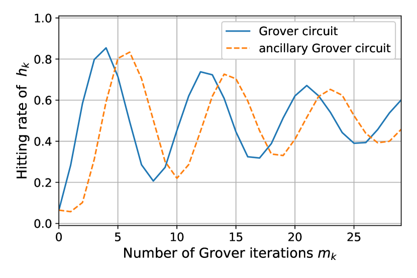
Figure 1: Experimental result of the probability of hitting “1”, as a function of the number of Grover iterations, $m_{k}=k$. The (blue) solid line is obtained from the Grover circuit of (2), and the (orange) dashed line is from the ancillary Grover circuit of (15). This experiment used the first and the fourth qubits of “ibm_kawasaki,” and $N_{\rm{shot}}=8192$ for both circuits.

We begin with defining a parametric distribution model under the unknown environment noise. Our basis is on the experimental result of the probability of hitting 1 as a function of the number of Grover iterations $m_{k}$, corresponding to Eq. (3) in the ideal case. The experiment was conducted using the IBM quantum device “ibm_kawasaki”, and the result is shown in the (blue) solid line in Fig. 1. This would suggest that we take a decayed oscillation

$$p_{\theta,\kappa}^{(k)}=\frac{1}{2}-\frac{1}{2}\mathrm{e}^{-\kappa m_{k}}\cos(2(2m_{k}+1)\theta).$$ (10)

Indeed this can be derived by assuming the depolarizing noise with strength $\kappa$; see [26]. Note that if $\kappa=0$, this is exactly Eq. (3). However, in reality there must exist some noise sources other than the depolarizing noise. Hence we introduce the following generalized model:

$$p_{\theta,\beta_{k}}^{(k)}=\frac{1}{2}-\frac{1}{2}\beta_{k}\cos(2(2m_{k}+1)\theta).$$ (11)

That is, a different type of noise, which is not necessarily the depolarizing noise, can be added to the system, depending on the number of iteration $m_{k}$. Note that Eq. (11) can be originated to the continuous-time model $p(t;\theta,\beta(t))=(1-\beta(t)\cos(2(2t+1)\theta))/2$ with $t$ the running time of the Grover operator; this is a semi parametric model with unknown function $\beta(t)$, which in our case is reduced to a finite-dimensional parametric model as only the finite number of sampling is performed.

The joint probability taken in the parallel strategy is given by

$$P(\mathbf{h};\theta,\boldsymbol{\beta})=\prod_{k={1}}^{M}[p_{\theta,\beta_{k}}^{(k)}]^{h_{k}}[1-p_{\theta,\beta_{k}}^{(k)}]^{1-h_{k}},$$ (12)

and the likelihood function becomes

$$L(\mathbf{H};\theta,\boldsymbol{\beta})=\prod_{j=1}^{N_{\rm{shot}}}P(\mathbf{h}^{j};\theta,\boldsymbol{\beta}),$$ (13)

where the meaning of $h_{k}$, $\mathbf{h}^{j}$, and $\mathbf{H}$ are the same as before. Therefore, the model distribution is parametrized by $\theta$ and the nuisance parameters $\boldsymbol{\beta}=(\beta_{1},\ldots,\beta_{M})$.

As mentioned before, we may fail to perfectly solve the optimization problem $\max_{\theta,\boldsymbol{\beta}}L(\mathbf{H};\theta,\boldsymbol{\beta})$ and obtain the ML estimator $\hat{\theta}_{\rm ML}$, especially when $M$ is large; this is indeed the motivation to apply the parameter orthogonalization method to remove $\boldsymbol{\beta}$. However, we cannot do this in a straightforward way, because, in this case, the model distribution is not regular; in fact, the number of outputs is $M$ while that of parameters is $M+1$, leading to the Fisher information matrix being degenerate.

Therefore we need to introduce an ancillary system that yields additional outputs, while keeping the number of noise parameters to recover the regularity of the model. In other words, we need a quantum circuit that is governed by the same noise as that on the entire Grover operation $\mathcal{G}^{m}$ and yet produces a different measurement outcome. For this purpose, we introduce the following “unamplified” operator $\mathcal{R}$:

$$\mathcal{R}:=-\mathcal{A}U_{0}\mathcal{A}^{\dagger}I_{n+1}.$$ (14)

This operator is obtained by replacing $\mathcal{U}_{f}=I_{n}\otimes\sigma_{z}$ by the identity operator $I_{n+1}$ in the Grover operator $\mathcal{G}=-\mathcal{A}\mathcal{U}_{0}\mathcal{A}^{\dagger}\mathcal{U}_{f}$. Note that, in quantum devices operated with the computational-basis measurement (i.e., measurement in the $Z$ basis), such as the current IBM superconducting devices, the $Z$ gate is implemented via the frame change; that is, no pulselike operation is performed on the system [37]. This technique has been applied to other types of quantum devices, such as NMR [38] and trapped ions [39]. Hence, it might be acceptable to assume that the operators $\mathcal{G}$ and $\mathcal{R}$ are subjected to the same noise. This basic assumption is supported in an experiment, as will be explained below.

Based on the above-introduced $\mathcal{R}$, we define the ancillary Grover circuit as follows; that is, we replace the last operation $\mathcal{G}$ of the entire Grover operations by $\mathcal{R}$. Then the final state in the ideal noiseless case is given by

$$\begin{split}\mathcal{R}\mathcal{G}^{m_{k}-1}\ket{\Psi}_{n+1}=&(-\mathcal{A}U_{0}\mathcal{A}^{\dagger})(-\mathcal{A}\mathcal{U}_{0}\mathcal{A}^{\dagger}\mathcal{U}_{f})\mathcal{G}^{m_{k}-2}\ket{\Psi}_{n+1}\\ =&\mathcal{U}_{f}\mathcal{G}^{m_{k}-2}\ket{\Psi}_{n+1}.\end{split}$$ (15)

For the realistic noisy case, the final state will be affected by the same noise through the above $m_{k}$ iterations, as that of $\mathcal{G}^{m_{k}}\ket{\Psi}_{n+1}$. Hence, the probability of getting 1 by measuring the last qubit of the circuit $\mathcal{R}\mathcal{G}^{m_{k}-1}$ under noise is, according to Eq. (11) and the fact that it is not affected by the operator $\mathcal{U}_{f}$, given by

$$\begin{split}q_{\theta,\beta_{k}}^{(k)}&=\frac{1}{2}-\frac{1}{2}\beta_{k}\cos(2(2(m_{k}-2)+1)\theta)\\ &=\frac{1}{2}-\frac{1}{2}\beta_{k}\cos(2(2m_{k}-3)\theta).\end{split}$$ (16)

This is the phase-delayed oscillation of Eq. (11), and this delay can be clearly seen in Fig. 1, showing with the (orange) dashed line the actual hitting ratio of 1 in the experiment. This result supports our assumption that the two circuits $\mathcal{G}^{m_{k}}$ and $\mathcal{R}\mathcal{G}^{m_{k}-1}$ are affected by the same noise.

The joint probability for ancillary circuits is given by

$$Q(\boldsymbol{\ell};\theta,\boldsymbol{\beta})=\prod_{k={1}}^{M}[q_{\theta,\beta_{k}}^{(k)}]^{\ell_{k}}[1-q_{\theta,\beta_{k}}^{(k)}]^{1-\ell_{k}},$$ (17)

and the likelihood function is constructed as

$$\begin{split}L(\mathbf{H},\mathbf{L};\theta,\boldsymbol{\beta})=\prod_{i=1}^{N_{\rm{shot}}}P(\mathbf{h}^{i};\theta,\boldsymbol{\beta})\prod_{j=1}^{N_{\rm{shot}}^{\prime}}Q(\mathbf{\boldsymbol{\ell}}^{j};\theta,\boldsymbol{\beta}),\end{split}$$ (18)

where $\mathbf{L}=\{\boldsymbol{\ell}^{1},\cdots,\boldsymbol{\ell}^{N_{\rm{shots}}^{\prime}}\}$ is the set of measurement results sampled from the binary random variables $\boldsymbol{\ell}=(\ell_{1},\cdots,\ell_{M})$, which follow the probability distributions of ancillary Grover circuits. Recall that the ancillary Grover circuit $\mathcal{R}\mathcal{G}^{m_{k}-1}$ is executed for $N_{\rm{shots}}^{\prime}$ times. Also with the help of an ancillary circuit, the corresponding Fisher information matrix can be invertible, meaning that certainly we now have the regular model to which the parameter orthogonalization method is applicable.

III.2 Orthogonalized parameters in MLAE

We can now apply the parameter orthogonalization method described in Sec. II.2 to our problem. The goal is to find the transformation such that the differential equation (9) is satisfied. For simplicity, we set $N_{\rm shot}=N_{\rm shot}^{\prime}$. In this setting, Eq. (9) is reduced to

$$\frac{\partial\beta_{k}(\boldsymbol{\xi})}{\partial\xi_{1}}\left(\frac{A_{k}^{p}(\xi_{1})}{1-A_{k}^{p}(\xi_{1})\beta_{k}^{2}(\boldsymbol{\xi})}+\frac{A_{k}^{q}(\xi_{1})}{1-A_{k}^{q}(\xi_{1})\beta_{k}^{2}(\boldsymbol{\xi})}\right)=-\frac{\beta_{k}(\boldsymbol{\xi})}{2}\left(\frac{1}{1-A_{k}^{p}(\xi_{1})\beta_{k}^{2}(\boldsymbol{\xi})}\frac{\partial A_{k}^{p}}{\partial\xi_{1}}+\frac{1}{1-A_{k}^{q}(\xi_{1})\beta_{k}^{2}(\boldsymbol{\xi})}\frac{\partial A_{k}^{q}}{\partial\xi_{1}}\right),$$

for all $k=1,2,\cdots,M$. Here we defined

$$A_{k}^{p}(\xi_{1})=\cos^{2}(2(2m_{k}+1)\xi_{1}),~{}~{}A_{k}^{q}(\xi_{1}) = \cos^{2}(2(2m_{k}-3)\xi_{1}).$$

Then we can prove that, for all $k=1,2,\cdots,M$, the function $\beta_{k}(\boldsymbol{\xi})$ satisfies

$$\{1-A_{k}^{p}(\xi_{1})\beta_{k}^{2}(\boldsymbol{\xi})\}\{1-A_{k}^{q}(\xi_{1})\beta_{k}^{2}(\boldsymbol{\xi})\}=c_{k}(\boldsymbol{\xi}^{\prime}),$$ (19)

where $c_{k}$ are arbitrary functions of the nuisance parameters $\boldsymbol{\xi}^{\prime}=(\xi_{2},\cdots,\xi_{M+1})$. Equation (19) can be solved as

$$\beta_{k}^{2}(\boldsymbol{\xi})=\frac{A_{k}^{p}(\xi_{1})+A_{k}^{q}(\xi_{1})\pm\sqrt{(A_{k}^{p}(\xi_{1})+A_{k}^{q}(\xi_{1}))^{2}-4A_{k}^{p}(\xi_{1})A_{k}^{q}(\xi_{1})(1-c_{k}(\boldsymbol{\xi}^{\prime}))}}{2A_{k}^{p}(\xi_{1})A_{k}^{q}(\xi_{1})}.$$ (20)

If $\beta_{k}(\boldsymbol{\xi})$ is a real function of $\boldsymbol{\xi}$ and $\beta_{k}(\boldsymbol{\xi})\geq 0$, the following condition needs to be satisfied;

$$1-\frac{(A_{k}^{p}(\xi_{1})+A_{k}^{q}(\xi_{1}))^{2}}{4A_{k}^{p}(\xi_{1})A_{k}^{q}(\xi_{1})}\leq c_{k}(\boldsymbol{\xi}^{\prime})\leq 1.$$

Thus, since $(A_{k}^{p}(\xi_{1})+A_{k}^{q}(\xi_{1}))^{2}/(4A_{k}^{p}(\xi_{1})A_{k}^{q}(\xi_{1}))\geq 1$, all solutions of $\beta_{k}(\boldsymbol{\xi})$ are real if $0\leq c_{k}(\boldsymbol{\xi}^{\prime})\leq 1$. Moreover, because $0\leq p^{(k)}_{\theta,\beta_{k}}\leq 1$ and $0\leq q^{(k)}_{\theta,\beta_{k}}\leq 1$, the following conditions need to be satisfied for all $k$:

$$0\leq A_{k}^{p}(\xi_{1})\beta_{k}^{2}(\boldsymbol{\xi})\leq 1,~{}~{}0\leq A_{k}^{q}(\xi_{1})\beta_{k}^{2}(\boldsymbol{\xi})\leq 1.$$

The relevant solution of $\beta_{k}(\boldsymbol{\xi})$ is thus

$$\beta_{k}(\boldsymbol{\xi})=\sqrt{\frac{A_{k}^{p}(\xi_{1})+A_{k}^{q}(\xi_{1})-\sqrt{(A_{k}^{p}(\xi_{1})+A_{k}^{q}(\xi_{1}))^{2}-4A_{k}^{p}(\xi_{1})A_{k}^{q}(\xi_{1})(1-c_{k}(\boldsymbol{\xi}^{\prime}))}}{2A_{k}^{p}(\xi_{1})A_{k}^{q}(\xi_{1})}}.$$ (21)

Recall from the theory of nuisance parameters shown in Sec. II B that, although $c_{k}(\boldsymbol{\xi}^{\prime})$ appearing in Eq. (21) is an arbitrary function satisfying $0\leq c_{k}(\boldsymbol{\xi}^{\prime})\leq 1$, it does not affect the estimation of $\theta=\xi_{1}$ in the asymptotic limit of a large number of measurements. Therefore by substituting $\beta_{k}(\boldsymbol{\xi})$ with roughly chosen $c_{k}(\boldsymbol{\xi}^{\prime})$ into the likelihood function (18) and solving the one-dimensional maximization problem with respect to $\theta=\xi_{1}$, we can efficiently and almost correctly compute the ML estimator for $\theta$. Lastly note that, if we eventually need to use a numerical solver for the differential equation (9), this means that the proposed method requires an additional computational resources, which has to be carefully compared to that of the multi-dimensional optimizer for the likelihood function (18). Moreover, such a numerical procedure may easily cause an error to the solutions $\beta_{k}(\boldsymbol{\xi})$ and the resulting likelihood function to be maximized with respect to $\theta$. Therefore, the fact that we have successfully obtained the analytic solution (21) is essentially important for the parameter orthogonalization method to gain the genuine computational advantage over the naive multi-parameter ML method.

IV Numerical and experimental demonstrations

In this section we study the performance of the proposed method in both numerical simulation and an experiment on a real superconducting quantum device.

IV.1 Numerical demonstration

First we numerically validate the parameter orthogonalization method in the non-asymptotic regime where the number of samples (measurement), i.e., $N_{\rm shot}$, is finite. More specifically, we study the solution of our likelihood equation with respect to $\theta=\xi_{1}$, i.e.,

$$\frac{\partial}{\partial\theta}\ln L(\mathbf{H},\mathbf{L};\theta,\boldsymbol{\beta})=0,$$ (22)

with $\beta_{k}(\boldsymbol{\xi})$ given by Eq. (21); then we will see if those solutions almost do not depend on $\xi_{k}$ or equivalently $c_{k}(\boldsymbol{\xi}^{\prime})$ for all $k\geq 2$, even when $N_{\rm shot}$ is relatively a small number. In fact, in the quantum computation scenario, $N_{\rm shot}$ should be kept as low as possible, hence this analysis is important.

The parameters of this numerical experiment are chosen as follows: The target value is $\theta_{*}=0.35$. The number of measurements (shots) is $N_{\rm{shot}}=50$ for both the Grover and the ancillary Grover circuits. The amplification schedule is $m_{k}=2^{k-1}~{}(k=1,2,\ldots,8)$. The true probability distribution is Eq. (10) with $\kappa=0.01$, which is used to generate the data; that is, only the depolarizing noise is added to the system, meaning that our parametric model can represent this true distribution by properly choosing $\beta_{k}$. Finally, as for the free parameters $\{c_{1},\ldots,c_{8}\}$ given in Eq. (20), we consider the following two cases:

$${\mathit{1}:} \{0.844,0.134,0.956,0.238,0.236,0.623,0.793,0.324\},$$

$${\mathit{2}:} \{0.571,0.452,0.475,0.259,0.107,0.965,0.362,0.522\}.$$

Figures 2(a) and 2(b) illustrate the shape of the log-likelihood function (18), with Case ${\mathit{1}}$ and Case ${\mathit{2}}$, respectively; recall that the other parameters are the same. They show that, in both cases, the optimal solution of Eq. (22), or equivalently the maximum point of the log-likelihood function, almost coincides with the target value $\theta_{*}=0.35$. That is, certainly the ML estimator is obtained by solving the one-dimensional maximization problem, without respect to the free parameters $\{c_{k}\}$. At the same time, the shape of the likelihood function implies that the conventional nine-dimensional likelihood function should have a very complicated landscape and as a result we may easily fail to obtain the ML estimator, which is indeed the main benefit of the parameter orthogonalization method.

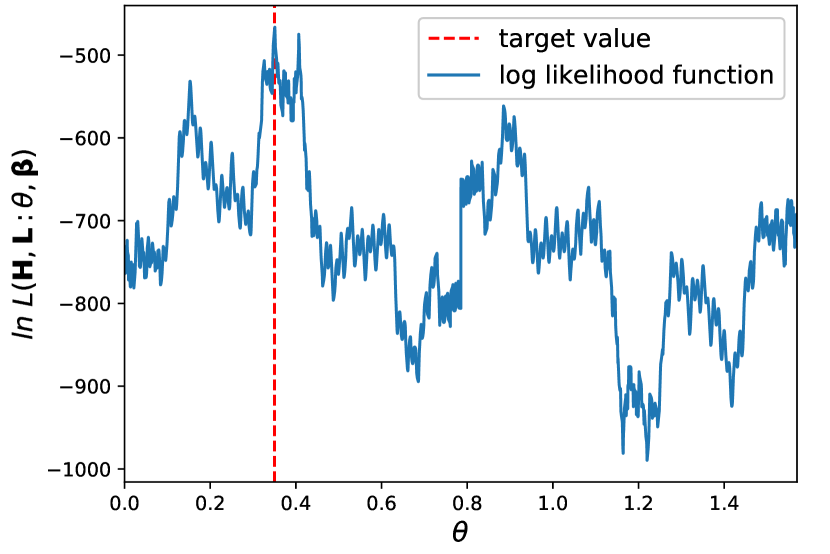
((a)) Case ${\mathit{1}}$

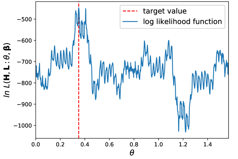
((b)) Case ${\mathit{2}}$

Figure 2: (Solid blue) Log likelihood function (18). (Dotted red) The target value $\theta_{*}=0.35$.

In addition to the optimal solution, the other critical points of $L(\mathbf{H},\mathbf{L};\theta,\boldsymbol{\beta})$, i.e., the solutions to Eq. (22), almost do not depend on $\{c_{k}\}$. Figure 3 shows the enlarged view of Figs. 2(a) and 2(b) at around the optimal point. Obviously, the shape of log-likelihood function changes depending on the two cases, but notably, their critical points look close to each other. There are small differences between those points of two functions due to the relatively small value of $N_{\rm shot}$, but we have observed that they become small by increasing $N_{\rm shot}$ as predicted by the theory.

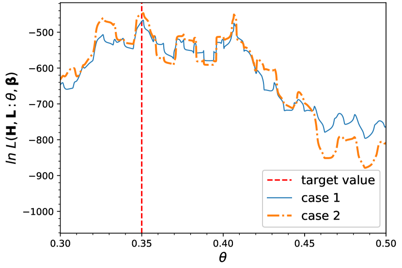
Figure 3: Enlarged view of Figs. 2(a) and 2(b).

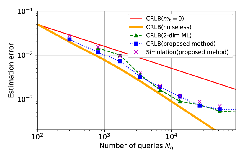
Figure 4: Estimation errors of $\theta_{*}$ vs the total number of queries $N_{q}$. The (red) thin and (yellow) thick lines are the CRLB for the classical method ($m_{k}=0$, i.e., the classical random sampling) and the quantum ML method without noise, respectively. The (green) dashed and (blue) dotted lines are the CRLB for the two-dimension ML estimator assuming the depolarizing noise and the proposed ML estimator, respectively. The (purple) cross marks are the standard deviation between the true value $\theta_{*}=0.35$ and the estimated values of $\theta$ computed using the proposed method.

Next we study the estimation performance of our ML estimator in the same setting as above except for the values of $\{c_{k}\}$. Figure 4 shows the estimation errors of the target value $\theta_{*}=0.35$, versus the total number of queries $N_{q}=\Sigma_{k=1}^{M}N_{\rm{shot}}(2m_{k}+1)$. The (red) thin and (yellow) thick lines are the CRLB for the classical method ($m_{k}=0$, i.e., the classical random sampling) and the quantum ML method without noise, respectively; the latter decreases the error quadratically faster than the former, as theoretically proven. The (green) dashed and (blue) dotted lines are the CRLB for the two-dimensional ML estimator assuming the depolarizing noise and the proposed ML estimator, respectively. Recall that those three ML estimators employ the operating schedule $m_{k}=2^{k-1}$. Also, our method makes $N_{\rm{shot}}=50$ measurements for both the Grover and the ancillary Grover circuits to construct the ML estimator, meaning that the number of measurements is $100$ for each $m_{k}$; hence for a fair comparison, the other ML estimators shown with the yellow solid and green dashed lines are assumed to make $100$ measurements for each $m_{k}$. In addition, the CRLB of the proposed method is calculated as the $(1,1)$ element of the inverse of the Fisher information matrix, which does not change before and after the parameter orthogonalization. The (purple) cross marks are the standard deviation between the true value $\theta_{*}=0.35$ and the estimated values of $\theta$ computed using our method which in this case take $c_{k}=0.3$ for all $k$.

The first notable point is that the green dashed line (the model assuming the depolarization) and the blue dotted line (the model not assuming the depolarization) are close with each other. Considering the fact that the true distribution is now subjected to only the depolarizing noise, this result means that our over-parametrized model can correctly capture the true distribution. Note that these CRLBs beat the classical estimation limit (the red thin solid line) up to a certain value of $N_{q}$, as theoretically predicted in [26]. Another important fact is that the estimation errors of the constructed estimator (the purple cross marks) well approximate the CRLB. That is, the estimator has the asymptotic consistency property, meaning that we are successfully solving the optimization problem and accordingly obtained the ML estimator almost correctly. This is clearly thanks to the advantage that the complicated nine-dimensional optimization problem now boils down to the one-dimensional one; the complicated shape of the likelihood function observed in Fig. 3 implies that the ML estimator maximizing the nine-dimensional function is hard to obtain, and as a result the gap between the purple cross marks and the blue dotted line can easily become large.

IV.2 Experiment on real quantum device

Here we show the result of an experiment conducted on IBM Quantum device “ibm_kawasaki,” to study how well our proposed estimator can actually manage the unidentifiable uncertainty arising in the real device. For this purpose we consider the problem of estimating the sum $S=\sum_{j=0}^{2^{n}-1}f(j)r(j)$ in the QAE framework [21, 26, 40]. In fact, $S$ can be encoded into the amplitude of a quantum state via the operator $\mathcal{A}=\mathcal{T}(\mathcal{P}\otimes I_{1})$ as follows;

$$\begin{split}\mathcal{A}\Ket{0}_{n}&\Ket{0}=\mathcal{T}\sum_{j}\sqrt{r(j)}\ket{j}_{n}\ket{0}\\ &=\sum_{j}\sqrt{r(j)}\ket{j}_{n}\left(\sqrt{f(j)}\ket{1}+\sqrt{1-f(j)}\ket{0}\right)\\ &=\sqrt{S}\ket{\tilde{\Psi}_{1}}\ket{1}+\sqrt{1-S}\ket{\tilde{\Psi}_{0}}\ket{0},\end{split}$$

where $\ket{\tilde{\Psi}_{1}}=\sum_{j}\sqrt{r(j)f(j)/S}\ket{j}_{n}$ and $\ket{\tilde{\Psi}_{0}}=\sum_{j}\sqrt{r(j)(1-f(j))/(1-S)}\ket{j}_{n}$. From Eq. (1), $S=\sin^{2}\theta$ can be efficiently estimated via QAE. In this paper, we consider $f(j)=\sin^{2}(\pi j/10)$ and $r(j)=1/2^{n}$ for $\forall j$, with $n=1$; in this case, $\mathcal{P}$ and $\mathcal{T}$ can be implemented using Hadamard and controlled $Y$-rotation gates. The true value is $\theta=0.175$ or equivalently $S=3.03\times 10^{-2}$. See [21, 26, 40] for a detailed description.

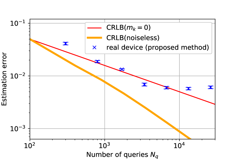
Figure 5: Estimation error of $\theta$ vs the total number of queries $N_{q}$. The thin red and thick yellow lines are the CRLB, obtained via the classical method, and the quantum ML method without noise, respectively. The blue cross marks are the standard deviation between the true value $\theta_{*}=0.175$ and the estimated values of $\theta$ that is experimentally computed using the proposed method.

For this estimation problem we apply the ML estimator with increasing number of Grover iterations as $m_{k}=2^{k-1}$, $(k=1,2,\ldots,7)$. Now our model assumes that a different noise is added to the system for different value of $m_{k}$; hence the model contains seven nuisance parameters $\boldsymbol{\beta}=(\beta_{1},\ldots,\beta_{7})$, which can be removed, however for constructing the ML estimator for $\theta$, using the parameter orthogonalization method. Figure 5 shows the result of estimation error versus the total number of queries, $N_{q}=\Sigma_{k=1}^{M}N_{\rm shot}(2m_{k}+1)$. The (red) thin solid line is the CRLB with $m_{k}=0$ (i.e., classical random sampling), and the (orange) thick solid line is the CRLB achieved by the ideal ML method with $m_{k}=2^{k}$. The (blue) cross marks are the standard deviation between the true value $\theta_{*}=0.175$ and the estimated values of $\theta$ obtained via the proposed method employing $c_{k}=0.3$ for $k=1,\cdots,7$. More specifically, the number of measurements is $N_{\rm shot}=50$ for both $\mathcal{G}^{m_{k}}$ and $\mathcal{R}\mathcal{G}^{m_{k}-1}$ to compute one $\hat{\theta}_{\rm ML}$; we repeated the same experiment $2,119$ times to compute the standard deviations (cross marks) and the three-times standard errors (error bars).

In the figure, we roughly see that the cross marks decrease with the quadratically enhanced scaling $N_{q}^{-1}$ (nearly parallel to the orange thick line) up to around $N_{q}=3\times 10^{3}$, although there is a constant-factor overhead. This overhead might be due to the additional uncertainty in the device as well as the bigger decay rate of the probability amplitude than $\kappa=0.01$ in the previous numerical simulation. Nevertheless, the cross mark at around $N_{q}=3\times 10^{3}$ is below the red line, meaning that the estimator is better than any classical means yet only at this point; unfortunately the estimation error does not decrease anymore, because excess noise is introduced by further iterating the Grover operation. In fact, we have confirmed that the noise level of “ibm_kawasaki” is comparable to that of “ibmq_valenica” used in the previous study [26], which also exhibited a similar saturation of the estimation error. These results imply that the one-dimensional maximization problem has been solved almost correctly, and the resulting ML estimator works pretty well even under the un-identifiable realistic noisy environment. Hence we have a perspective that the proposed model, which does not incorporate a specific noise characteristic, may be able to capture a more complicated larger-dimensional system by increasing the number of nuisance parameters $\{\beta_{k}\}$ and, thanks to the parameter orthogonalization, the ML estimator may still be computed almost exactly without respect to $\{\beta_{k}\}$.

V Conclusion

Quantum computing can be regarded as a system that encodes and processes some quantities (parameters) of interest in a real physical device which are finally retrieved and estimated as precisely as possible. However, for the time being we will have to play with devices under unknown noise environment. The statistical estimation theory provides a useful toolbox for dealing with such a practical estimation problem, and in our view, its role will remain or even become bigger when those devices acquire some level of fault tolerance in the future. The nuisance parameters method presented in this paper is one such useful tool. Recall that what was presented in this paper is not a blind application of the nuisance parameters method; for instance, we need an additional quantum circuit (called the ancillary Grover circuit) to apply the theory and thereby construct an estimator without respect to the nuisance parameters. Also, it was somewhat surprising that we can analytically solve the differential equation (9) in our problem; as emphasized before, this is indeed a key result obtained in this paper, because otherwise (i.e., if the solution has to be numerically computed) the parameter orthogonalization procedure may bring a significant computational overhead.

Extension to the method formulated within the semi parametric estimation theory is clearly an important next step of this work. Also, it should be desirable if such an extension could cover the problem of quantum phase estimation, which is also an important subroutine in many quantum algorithms.

APPENDIX

Here we show that, if the new parameters satisfy the differential equation (9), then the $(1,k)$-element of the new Fisher information matrix $J_{\xi}$ becomes zero for $k=2,3,\dots,M+1$ [31].

First, we use the symbol $\tau$ to explicitly represent the variable transformation:

$$\theta =\tau_{0}(\xi_{1})=\xi_{1},~{}$$

$$\beta_{1} =\tau_{1}(\xi_{1},\xi_{2},\xi_{3},\cdots,\xi_{M+1}),$$

$$\beta_{2} =\tau_{2}(\xi_{1},\xi_{2},\xi_{3},\cdots,\xi_{M+1}),$$

$$\vdots$$

$$\beta_{M} =\tau_{M}(\xi_{1},\xi_{2},\xi_{3},\cdots,\xi_{M+1}).$$

Also, to make the notation simple, we define $f=\log p(x;\theta,\boldsymbol{\beta})$ and $g=\log p(x;\boldsymbol{\xi})$. We now calculate $(J_{\xi})_{1,k}$ for $k=2,3,\dots,M+1$ using the chain rule as follows:

$$(J_{\xi})_{1,k} ={\mathbb{E}}\Big{[}\frac{\partial g}{\partial\xi_{1}}\frac{\partial g}{\partial\xi_{k}}\Big{]}={\mathbb{E}}\Big{[}\Big{(}\frac{\partial f}{\partial\theta}\frac{\partial\tau_{0}}{\partial\xi_{1}}+\sum_{h=2}^{M+1}\frac{\partial f}{\partial\beta_{h-1}}\frac{\partial\tau_{h-1}}{\partial\xi_{1}}\Big{)}\Big{(}\frac{\partial f}{\partial\theta}\frac{\partial\tau_{0}}{\partial\xi_{k}}+\sum_{i=2}^{M+1}\frac{\partial f}{\partial\beta_{i-1}}\frac{\partial\tau_{i-1}}{\partial\xi_{k}}\Big{)}\Big{]}$$

$$={\mathbb{E}}\Big{[}\Big{(}\frac{\partial f}{\partial\theta}+\sum_{h=2}^{M+1}\frac{\partial f}{\partial\beta_{h-1}}\frac{\partial\tau_{h-1}}{\partial\xi_{1}}\Big{)}\Big{(}\sum_{i=2}^{M+1}\frac{\partial f}{\partial\beta_{i-1}}\frac{\partial\tau_{i-1}}{\partial\xi_{k}}\Big{)}\Big{]}=\sum_{i=2}^{M+1}\frac{\partial\tau_{i-1}}{\partial\xi_{k}}{\mathbb{E}}\Big{[}\Big{(}\frac{\partial f}{\partial\theta}+\sum_{h=2}^{M+1}\frac{\partial f}{\partial\beta_{h-1}}\frac{\partial\tau_{h-1}}{\partial\xi_{1}}\Big{)}\frac{\partial f}{\partial\beta_{i-1}}\Big{]}$$

$$=\sum_{i=2}^{M+1}\frac{\partial\tau_{i-1}}{\partial\xi_{k}}\Big{(}{\mathbb{E}}\Big{[}\frac{\partial f}{\partial\theta}\frac{\partial f}{\partial\beta_{i-1}}\Big{]}+\sum_{h=2}^{M+1}{\mathbb{E}}\Big{[}\frac{\partial f}{\partial\beta_{i-1}}\frac{\partial f}{\partial\beta_{h-1}}\Big{]}\frac{\partial\tau_{h-1}}{\partial\xi_{1}}\Big{)}=\sum_{i=2}^{M+1}\frac{\partial\tau_{i-1}}{\partial\xi_{k}}\Big{(}J_{1,i}+\sum_{h=2}^{M+1}J_{i,h}\frac{\partial\tau_{h-1}}{\partial\xi_{1}}\Big{)}.$$

Therefore if

$$J_{1,i}+\sum_{h=2}^{M+1}J_{i,h}\frac{\partial\tau_{h-1}}{\partial\xi_{1}}=0$$

for $i=2,3,\dots,M+1$, then we have $(J_{\xi})_{1,k}=0$.

References

- Grover [1998] L. K. Grover, Quantum computers can search rapidly by using almost any transformation, Phys. Rev. Letters 80, 4329 (1998).
- Brassard et al. [2002] G. Brassard, P. Hoyer, M. Mosca, and A. Tapp, Quantum amplitude amplification and estimation, Contemporary Mathematics 305, 53 (2002).
- Montanaro [2015] A. Montanaro, Quantum speedup of Monte Carlo methods, Proceedings of the Royal Society A: Mathematical, Physical and Engineering Sciences 471 (2015).
- Rebentrost et al. [2018] P. Rebentrost, B. Gupt, and T. R. Bromley, Quantum computational finance: Monte Carlo pricing of financial derivatives, Phys. Rev. A 98, 022321 (2018).
- Woerner and Egger [2019] S. Woerner and D. J. Egger, Quantum risk analysis, npj Quantum Information 5, 1 (2019).
- Stamatopoulos et al. [2020] N. Stamatopoulos, D. J. Egger, Y. Sun, C. Zoufal, R. Iten, N. Shen, and S. Woerner, Option pricing using quantum computers, Quantum 4, 291 (2020).
- Martin et al. [2021] A. Martin, B. Candelas, Á. Rodríguez-Rozas, J. D. Martín-Guerrero, X. Chen, L. Lamata, R. Orús, E. Solano, and M. Sanz, Toward pricing financial derivatives with an ibm quantum computer, Phys. Rev. Research 3, 013167 (2021).
- Egger et al. [2020] D. J. Egger, R. Garcia Gutierrez, J. Cahue Mestre, and S. Woerner, Credit risk analysis using quantum computers, IEEE Transactions on Computers 70, 2136 (2020).
- Miyamoto and Shiohara [2020] K. Miyamoto and K. Shiohara, Reduction of qubits in a quantum algorithm for monte carlo simulation by a pseudo-random-number generator, Phys. Rev. A 102, 022424 (2020).
- Kaneko et al. [2021] K. Kaneko, K. Miyamoto, N. Takeda, and K. Yoshino, Quantum speedup of monte carlo integration with respect to the number of dimensions and its application to finance, Quantum Information Processing 20, 185 (2021).
- Chakrabarti et al. [2021] S. Chakrabarti, R. Krishnakumar, G. Mazzola, N. Stamatopoulos, S. Woerner, and W. J. Zeng, A threshold for quantum advantage in derivative pricing, Quantum 5, 463 (2021).
- Miyamoto [2021] K. Miyamoto, Bermudan option pricing by quantum amplitude estimation and chebyshev interpolation, arXiv:2108.09014 (2021).
- Huang et al. [2020] H.-L. Huang, D. Wu, D. Fan, and X. Zhu, Superconducting quantum computing: a review, Science China Information Sciences 63, 1 (2020).
- Stehli et al. [2020] A. Stehli, J. D. Brehm, T. Wolz, P. Baity, S. Danilin, V. Seferai, H. Rotzinger, A. V. Ustinov, and M. Weides, Coherent superconducting qubits from a subtractive junction fabrication process, Applied Physics Letters 117, 124005 (2020).
- Häffner et al. [2008] H. Häffner, C. F. Roos, and R. Blatt, Quantum computing with trapped ions, Physics reports 469, 155 (2008).
- He et al. [2019] Y. He, S. Gorman, D. Keith, L. Kranz, J. Keizer, and M. Simmons, A two-qubit gate between phosphorus donor electrons in silicon, Nature 571, 371 (2019).
- Wang et al. [2021] G. Wang, D. E. Koh, P. D. Johnson, and Y. Cao, Minimizing estimation runtime on noisy quantum computers, PRX Quantum 2, 010346 (2021).
- Veldhorst et al. [2015] M. Veldhorst, C. H. Yang, J. C. C. Hwang, W. Huang, J. P. Dehollain, J. T. Muhonen, S. Simmons, A. Laucht, F. E. Hudson, K. M. Itoh, A. Morello, and A. S. Dzurak, A two-qubit logic gate in silicon, Nature 526, 410 (2015).
- Bruzewicz et al. [2019] C. D. Bruzewicz, J. Chiaverini, R. McConnell, and J. M. Sage, Trapped-ion quantum computing: Progress and challenges, Applied Physics Reviews 6, 021314 (2019).
- Jurcevic et al. [2021] P. Jurcevic, A. Javadi-Abhari, L. S. Bishop, I. Lauer, D. F. Bogorin, M. Brink, L. Capelluto, O. Gunluk, T. Itoko, N. Kanazawa, A. Kandala, G. A. Keefe, K. Krsulich, W. Landers, E. P. Lewandowski, D. T. McClure, G. Nannicini, A. Narasgond, H. M. Nayfeh, E. Pritchett, M. B. Rothwell, S. Srinivasan, N. Sundaresan, C. Wang, K. X. Wei, C. J. Wood, J.-B. Yau, E. J. Zhang, O. E. Dial, J. M. Chow, and J. M. Gambetta, Demonstration of quantum volume 64 on a superconducting quantum computing system, Quantum Science and Technology 6, 025020 (2021).
- Suzuki et al. [2020a] Y. Suzuki, S. Uno, R. Raymond, T. Tanaka, T. Onodera, and N. Yamamoto, Amplitude estimation without phase estimation, Quantum Information Processing 19, 75 (2020a).
- Aaronson and Rall [2020] S. Aaronson and P. Rall, Quantum approximate counting, simplified, in Symposium on Simplicity in Algorithms (SIAM, 2020) pp. 24–32.
- Grinko et al. [2021] D. Grinko, J. Gacon, C. Zoufal, and S. Woerner, Iterative quantum amplitude estimation, npj Quantum Information 7, 52 (2021).
- Nakaji [2020] K. Nakaji, Faster amplitude estimation, Quantum Inf. Comput. 20, 1109 (2020).
- Brown et al. [2020] E. G. Brown, O. Goktas, and W. Tham, Quantum amplitude estimation in the presence of noise, arXiv:2006.14145 (2020).
- Tanaka et al. [2021] T. Tanaka, Y. Suzuki, S. Uno, R. Raymond, T. Onodera, and N. Yamamoto, Amplitude estimation via maximum likelihood on noisy quantum computer, Quantum Information Processing 20, 293 (2021).
- Uno et al. [2021] S. Uno, Y. Suzuki, K. Hisanaga, R. Raymond, T. Tanaka, T. Onodera, and N. Yamamoto, Modified grover operator for quantum amplitude estimation, New Journal of Physics 23, 083031 (2021).
- Giurgica-Tiron et al. [2020] T. Giurgica-Tiron, I. Kerenidis, F. Labib, A. Prakash, and W. Zeng, Low depth algorithms for quantum amplitude estimation, arXiv:2012.03348 (2020).
- Plekhanov et al. [2021] K. Plekhanov, M. Rosenkranz, M. Fiorentini, and M. Lubasch, Variational quantum amplitude estimation, arXiv:2109.03687 (2021).
- Giurgica-Tiron et al. [2021] T. Giurgica-Tiron, S. Johri, I. Kerenidis, J. Nguyen, N. Pisenti, A. Prakash, K. Sosnova, K. Wright, and W. Zeng, Low depth amplitude estimation on a trapped ion quantum computer, arXiv:2109.09685 (2021).
- Cox and Reid [1987] D. R. Cox and N. Reid, Parameter orthogonality and approximate conditional inference, Journal of the Royal Statistical Society: Series B (Methodological) 49, 1 (1987).
- Begun et al. [1983] J. M. Begun, W. Hall, W.-M. Huang, and J. A. Wellner, Information and asymptotic efficiency in parametric-nonparametric models, The Annals of Statistics 11, 432 (1983).
- Suzuki [2020] J. Suzuki, Nuisance parameter problem in quantum estimation theory: tradeoff relation and qubit examples, Journal of Physics A: Mathematical and Theoretical 53, 264001 (2020).
- Suzuki et al. [2020b] J. Suzuki, Y. Yang, and M. Hayashi, Quantum state estimation with nuisance parameters, Journal of Physics A: Mathematical and Theoretical 53, 453001 (2020b).
- Tsang et al. [2020] M. Tsang, F. Albarelli, and A. Datta, Quantum semiparametric estimation, Phys. Rev. X 10, 031023 (2020).
- Cimini et al. [2021] V. Cimini, F. Albarelli, I. Gianani, and M. Barbieri, Semiparametric estimation in hong-ou-mandel interferometry, arXiv:2109.09368 (2021).
- McKay et al. [2017] D. C. McKay, C. J. Wood, S. Sheldon, J. M. Chow, and J. M. Gambetta, Efficient Z gates for quantum computing, Phys. Rev. A 96, 022330 (2017).
- Knill et al. [2000] E. Knill, R. Laflamme, R. Martinez, and C.-H. Tseng, An algorithmic benchmark for quantum information processing, Nature 404, 368 (2000).
- Knill et al. [2008] E. Knill, D. Leibfried, R. Reichle, J. Britton, R. B. Blakestad, J. D. Jost, C. Langer, R. Ozeri, S. Seidelin, and D. J. Wineland, Randomized benchmarking of quantum gates, Phys. Rev. A 77, 012307 (2008).
- Tanaka et al. [2019] T. Tanaka, S. Uno, Y. Suzuki, and R. Raymond, https://github.com/Qiskit/qiskit-community-tutorials/blob/master/algorithms/SimpleIntegral_AEwoPE.ipynb (2019), accessed: 2021-10-01.