Do photon-number-resolving detectors provide
valid evidence for the discrete nature of light?

Abstract

We consider the question of whether photon-number-resolving (PNR) detectors provide compelling evidence for the discrete nature of light; i.e., whether they indicate the prior presence of a certain number of discrete photons. To answer this question, we reveal the insufficient signal-to-noise ratio (SNR) of existing PNR detectors, and propose an alternative interpretation for the analysis of PNR detector output that is consistent with a wave picture of light and does not rely on the presumption of light particles. This interpretation is based on the aggregation of correlated or accidentally coincident detections within a given detector coincidence window. Our interpretation accounts for the arbitrary character of detector coincidence windows and includes connections to established treatments of intensity interferometers. To validate our interpretation, we performed an experiment on a multiplexed PNR detector and examined the dependence of photon number on the coincidence window via post-processing. These observations were then compared to a fully classical wave model based on amplitude threshold detection, and the results were found to be in excellent agreement. We find that results from low SNR PNR detectors, such as those existing in the literature, are able to be described by classical descriptions, and therefore do not demonstrate evidence for the discrete nature of light.

I Introduction

In recent times, Einstein’s postulate of light quanta has endured unquestioned by all but a few cautious investigators. It is no wonder since these days we have PNR detectors which very clearly and plainly demonstrate the particle nature of light by the multimodal structure of photon statistics. What could this characteristic intimate other than the particle nature of light? The bubble paradox, another of Einstein’s gedanken experiments, exhibits the conundrum of light particle locality, energy conservation, and quantum state collapse. The connection between this gedanken experiment and PNR detectors is particularly illustrative and worth revisiting at the end of this work.

In the generally accepted interpretation of photon-number-resolving (PNR) detectors, the multimodal output of the detectors has been deemed to be prima facie evidence for light particles. The success of linear quantum optical computing [1, 2] as well as the security certification for quantum networks [3] relies on this interpretation of PNR detectors. PNR detectors utilize simultaneous detections of photons to gather information on input photon states. Various states of light from appropriate sources can be detected by PNR detectors which, in turn, output the photon number distribution of the input light, a crucial measure for exploiting the unique qualities of quantum light [4]. Needless to say, an acceptable signal-to-noise ratio (SNR) is paramount for accurately resolving photon number. Typical calculations of the SNR of PNR detectors are encapsulated by the ratio of light counts to dark counts. However, an additional source of noise constituted by so-called “accidental coincidences” manifests in calculations of SNR for intensity interferometers (IIs). In this work, we argue that due to the similarity in design and operation of PNR detectors and IIs, that accidental coincidences should be incorporated in SNR computations for PNR detectors.

It is safe to say that the stance for the existence of light particles in its dualistic form has been the prevalent view since the first quarter of the 20^th century [5, 6]. Blackbody radiation, and the photoelectric and Compton effects were the first three phenomena constituting evidence that the electromagnetic field is quantized. More subtle effects found later solidified this position such as spontaneous emission, the Hanbury Brown and Twiss effect,[7] the Hong-Ou Mandel effect,[8] etc. However, in 1963 Sudarshan noted the equivalence between the semiclassical and quantized field descriptions of statistical light beams.[9] Several years later Lamb and Scully derived a semiclassical model where the field is treated classically while the detector is marked by quantized behavior. In this way, the photoelectric effect, previously interpreted as evidence of a quantized light field could also, in fact, be seen as evidence of a semiclassical paradigm.[10] Moreover, since Lamb and Scully’s semiclassical model, the aforementioned phenomena have lost their status as exclusively explained by a light particle picture.[11, 12, 13, 14, 15, 16]

The measurement of correlations between detectors has occupied a pivotal position in the field of quantum optics in no small part due to its crucial role as a powerful method for extracting experimental evidence concerning the degree of optical coherence of a system.[17, 18, 19] The work of Hanbury Brown and Twiss largely founded the practice of such correlation measurements [20, 7, 21]. The IIs used in their work incorporated pairs of detectors to measure correlations ($g^{(2)}$), thereby quantifying the degree of spatial coherence of stellar sources as a function of detector separation. This technique was used to successfully ascertain the angular dimension of the sources.

Generalizations to higher numbers of detectors and, as such, access to higher order correlations has been explored theoretically by Malvimat et al. [22]. They found that the SNR (in dB) of a generalized intensity interferometer using $N$ Geiger-mode single-photon detectors scales as

$$10^{\mathrm{SNR}/10}\sim\frac{N(N-1)}{2}(r\Delta t)^{N/2}\frac{\Delta\tau}{\Delta t}\sqrt{\frac{T}{\Delta t}}\;,$$ (1)

where $r$ is the detection rate, $\Delta t$ is the reciprocal electrical bandwidth or, equivalently, the coincidence window, $\Delta\tau$ is the source coherence time, and $T$ is the integration time. The symbol $\sim$ reflects the lack of precision of the expression due to individual characteristics of a particular measurement setup, such as detector efficiency and transmission losses. Accidental coincidences, in contrast to correlated coincidences, constitute the most elusive source of noise to overcome in the case of correlated measurements, as other sources of noise, such as dark counts and afterpulsing, can be compensated straightforwardly at the individual detector level of analysis. Accidental coincidences take multiple forms including dark-count-dark-count combinations between constituent detectors or (effective) pixels, dark-count-light-count combinations, and light count combinations between different coherence times, but within single coincidence windows, i.e. when $\Delta t\gg\Delta\tau$. (The accidental coincidences caused by the mismatch between coherence time and coincidence window establish the primary cause contributing to coincidence window dependence of photon statistics shown later in this work.) The quantity $r\Delta t$ is always less than unity in experiments, since the detector dead (recovery or reset) time is at least as long as the coincidence window. The condition $r\Delta t<1$ implies that the SNR decreases as the number of detectors increase, and this property has discouraged their use in II experiments.

Despite being separated by the fields of astronomy and quantum optics, intensity interferometers show a striking resemblance to certain multiplexed PNR detectors. In fact, an intensity interferometer, when operated using Geiger-mode detectors, has exactly the same architecture as a two-detector multiplexed PNR detector. Furthermore, the similitude persists if we extrapolate the architecture to $N$ detectors. Not only is the layout topologically equivalent, but the technical analysis revealing correlations by grouping coincident detections in IIs is essentially the same as counting photon number by grouping coincident detections in PNR detectors.

This compelling similitude suggests that the prevailing method of calculating SNR for PNR detectors may be neglecting the more subtle source of noise from accidental coincidences, which by contrast is included for IIs. If so, it would be prudent to question the certitude with which PNR detector results are presented. It also suggests that certain anomalous characteristics (such as coincidence window dependent photon statistics) may manifest if accidental coincidences dominate PNR detector results. Figure 1 shows the dependence of SNR on both coincidence window and number of single photon detectors (therefore number of incident photons). The red box represents the parameter space explored experimentally in this work. The white dashed line signifies a limit of effectiveness for PNR detectors beyond which detector number saturation, to be described below, spoils results. For the sake of clarity, the experimental results conducted in this work are not meant to solve the issue of accidental coincidences, as is evidenced by the insufficient SNR shown in the red box in Figure 1. Rather, we demonstrate that one of the anomalous characteristics associated with high rates of accidental coincidences, i.e. having a low SNR, is the coincidence window dependence of photon statistics. This low SNR is representative of many PNR detectors surveyed below, and suggests similar anomalous characteristics may be observed in existing devices.

At this juncture a distinction must be made between what we may call detector temporal saturation and PNR detector number saturation. Detector temporal saturation is the limitation in which the count rate of a single-photon detector in Geiger mode fails to be as sensitive to detections at higher intensities as it is at lower intensities. The single photon detector count rate peaks at a maximum count number as input power is increased. The maximum count rate, which characterizes detector temporal saturation, is inversely proportional to the detector dead time. PNR detector number saturation, in marked difference, occurs when every discrete detector (or effective pixel) composing the PNR detector is continuously activated, and therefore practically insensitive to incoming light. This condition is reflected in Eqn. (1) as $N\approx r\Delta t$ and is represented by the white dashed line in Fig. 1. In practice, this condition implies that SNR values in the region to the right of the white dashed line are inaccessible due to PNR detector number saturation, which happens independently of detector temporal saturation.

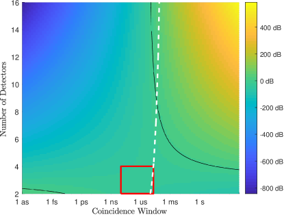
Figure 1: (Color online) Theoretical signal-to-noise ratio for $N$-detector intensity interferometers. The black contour indicates an SNR of 3 dB. The parameters used in the expression match the experimental conditions used in this work: 2 ps coherence time, 200 kcps detection rate, a 0.5 second integration time. The red box displays the area experimentally explored in this work. The white dashed line represents detector number saturation, to the right of which none of the detectors composing the PNR detector are able to fully reset.

One clear characteristic of Fig. 1, owing to the condition $r\Delta t<1$, is the precipitous falloff of the SNR with increasing detector number. With these experimental parameters, an SNR higher than the 3-dB threshold level (shown by the black line) is reflected only for correlations of order two (which occur at coincidence windows less than 1 fs). Unfortunately, the signal for higher order correlations is overwhelmed by accidental coincidences. Cognizance of such SNR relations is crucial to avoid mistaking accidental coincidences for correlated coincidences.

II Review of PNR Detectors

As mentioned above, many existing studies on PNR detectors belie a low SNR when calculated using Eqn. 1. Figure 2 shows the SNR results of a survey of PNR detectors calculated using parameters listed in their respective text.

In this work, we focus on the following most utilized PNR detector architectures: visible light photon counters (VLPCs) [24, 25, 26, 27, 28], transition edge sensors (TESs) [29, 30, 31, 32, 33, 34, 35, 36, 37, 38, 39, 40], superconducting nanowire single-photon detectors (SNSPDs) [41, 42, 43, 44, 45, 46, 47], and a class of noncryogenic detectors (NCDs) of which the following three general sub-types exist: beam splitter single photon detectors (BS-SPDs) [48, 49, 50],, and spatially [52, 53, 54, 55, 56] or temporally [57] multiplexed designs. In addition, unique PNR detector designs also exist [58, 59, 60].

Figure 2 shows that SNR typically decreases as a function of increasing detector number (or photon number equivalently). Three detectors (two TESs and one NCD) manage to achieve an SNR above 3 dB for 2 photon events, however, all rapidly decrease with only one TES remaining above 3 dB for 3 photon events. As one can see, the vast majority of PNR detectors fall below the 3 dB threshold for SNR. At these low SNR values results would be dominated by accidental coincidences.

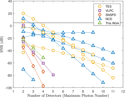
Figure 2: (Color online) Survey of theoretical signal-to-noise ratio for PNR detectors using $N$-detector intensity interferometry treatment and individually stated device parameters. Various types of PNR detectors are represented in the survey including, transition edge sensors (TES), visible light photon counters (VLPC), superconducting nanowire single photon detector based devices (SNSPD), various noncryogenic detectors (NCD), lastly this work, a member of the noncryogenic type, is shown in green in the midst of the detectors. Few PNR detectors achieve an acceptable SNR even at low photon numbers.

In addition to the SNR decline, the arbitrary nature of the coincidence window for PNR detectors breeds suspicion with regards to the standard interpretation of photon counting. In order to fully grasp the importance of arbitrary coincidence windows and their effects on photon statistics we briefly review some aspects of current PNR detectors.

Simultaneous detection is an ingredient critical to the intended operation of PNR detectors and is vital to probing the veracity of multiphoton states. “In the elementary quantum process of decay of a photon ($\omega_{p}$) into two new photons ($\omega_{1}$, $\omega_{2}$), emission of the products should be simultaneous.” [61] Therefore, detection, barring a relative delay line, should be simultaneous. As noted by Grangier et al., one stipulation of this deduction is that the coincidence window chosen for detection must be no greater than the coherence time of the source [62, 63]. This stipulation ensures that more true coincident detections occur in the detection area rather than accidental uncorrelated detections. This condition is ostensibly borrowed from SNR concerns when dealing with IIs. For PNR detectors, if the coherence time is shorter than the coincidence window, we would expect accidental uncorrelated detections to aggregate within coincidence windows and therefore artificially increase the calculated photon number as the coincidence window increases. A test of this behavior would be to vary the coincidence window while keeping the source power constant. In this work we address this test by systematically exploring the parameter space comprised of coincidence window duration and input power for a coherent source. However, even if the coincidence window is matched to the coherence time there is still a scaling problem if one increases the number of detectors to capture higher order states, as we have seen in Fig. 1.

PNR detectors are characterized by several different metrics, such as efficiency, dead time, maximum detectable photon number, photon number resolution, etc. The coincidence window is an often overlooked metric characterizing each particular PNR detector. Coincidence windows are given a warranted amount of attention for Bell inequality experiments [64, 65] but are largely neglected for PNR detectors. Obviously, coincidence windows exist in devices regardless of their lack of intentional design in sensor architecture and construction; they are often hardware defined and associated with the slowest response circuitry in the sensor, typically the amplifier system. Oftentimes, the effective coincidence window is merely the reciprocal electrical bandwidth. In this work, we define the coincidence window as the timescale that determines if one or more detector triggerings should be grouped together, thereby indicating that the detections should be thought of as having a previous association. Already we can see that judgement is an explicit factor in the choice of a coincidence window. In this vein, a software-defined coincidence window, whose only limitation is the hardware circuitry speed, can be tuned to maximize visibility or other metrics of interest [62].

In the case of a hardware-defined coincidence window, the coincidence window is the timescale that characterizes the pileup behavior of the sensor response signal and determines to a large degree how the combination of discrete height pulses in the response signal histogram are distributed. Liao et al. [66] have shown changes in photon statistics while increasing power (keeping the coincidence window constant). In this work we vary not only the power of our coherent source, but also the coincidence window.

If elicited, a shift in the photon number distribution caused by merely changing the coincidence window would raise suspicions regarding the accuracy and consistency of the PNR detector in question. Independence of photon number distribution from the coincidence window is regularly and tacitly assumed, perhaps with a vague stipulation that the coincidence window should be small enough. As we show in this paper with a beamsplitter-based multiplexed PNR detector with admittedly low SNR, the calculated photon number distribution is artificially and strongly dependent upon the coincidence window. In light of this, there is a need for a logically consistent interpretation governing the validity of coincidence window choices with the goal of developing the capability to certify valid PNR results.

As we have alluded, in addition to the coincidence window, the coherence time of the light source is pivotal to the proper interpretation of statistical light distributions measured by PNR detectors. Lasers and spontaneous parametric down conversion (SPDC) crystals are two of the most common sources for probing the performance characteristics of PNR detectors. Coherence times for lasers range from 1 ps for entry-level scientific lasers to over 1 ms for high performance, ultra-narrow bandwidth lasers. On the other hand, SPDC source coherence times range from 80 ps for unfiltered output [67] to 2 $\mu$s for high performance sources [68]. The atomic cascade source used by Grangier et al. for studies on anticorrelation, for example, possessed a lifetime of 4.7 ns [62]. It stands to reason that the stipulation that coincidence windows be no greater than the source coherence time should not only apply to intensity interferometers but also to PNR detectors. Experimental endeavors have demonstrated that an implicit policy of minimizing the coincidence window seems to be in effect, which would be the correct objective to some degree for increasing SNR according to Fig. 1. However, detector coincidence windows are rarely, if ever, mentioned in comparison to source coherence time, which would be the relevant scaling criterion for determining the suitability of a particular coincidence window. Furthermore, coincidence window minimization across different PNR detector modalities and designs stretches across six orders of magnitude, as shown in Fig. 3, increasing the inconsistency with which photon statistics are surmised. Again, we emphasize that given a coincidence window no greater than the source coherence time, SNR scaling issues persist for higher numbers of detectors and therefore detection of higher order multiphoton states.

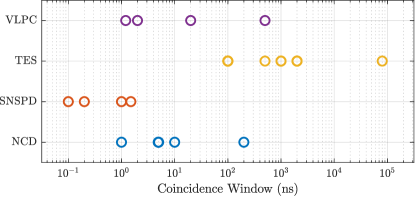
Figure 3: (Color online) Survey of coincidence windows for the most relevant PNR detectors including visible light photon counters (VLPC), transition edge sensors (TES), superconducting nanowire single-photon detectors (SNSPD), and noncryogenic detectors (NCD) consisting of spatially and temporally multiplexed single photon detectors and a modified avalanche photodiode.

To our knowledge no consistent method has been used in these works to establish an optimal coincidence window other than minimization. Since most experimental setups have used the smallest coincidence window available, we are limited only to raising the coincidence window above the hardware defined level, in our case by using a software-defined coincidence window longer than the hardware-defined level of 1 ns.

III Experimental Setup

The PNR detector used in this work consists of a multiplexed beamsplitter tree-based network with three 50:50 beamsplitters (Thorlabs CCM5-BS017) supplying four independent single-photon detectors (S-fifteen Si-APD). A fiber-based laser diode (Thorlabs MCLS1 with ss-d6-6-785-50 diode) supplies the input coherent light at 778 nm with a coherence time of 2 ps. An in-line fiber variable attenuator (Thorlabs VOA780-APC), fiber coupling (Thorlabs PAF2-2B), and a set of neutral density filters (Thorlabs NEK01) provide coupling to free space and attenuation. Timing electronics (S-fifteen TDC1) provided timestamps of all detection events among the four detectors, with a timestamp step of 1 ns and a timing resolution of 2 ns. The software-defined coincidence window was swept from 20 $\mu$s down to 10 ns in 500-ns steps. Power was measured using a free-space power meter(Newport 843-R), which could be positioned to intersect the optical axis before the attenuation stack.

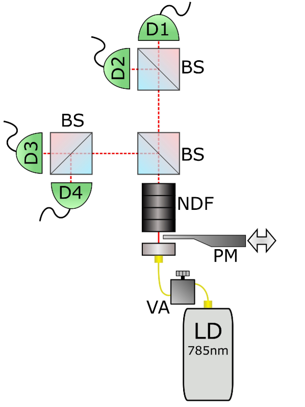
Figure 4: (Color online) The experimental setup consists of four single-photon detectors (D1–D4), three 50/50 beamsplitters (BS), several neutral density filters (NDF), a laser diode (LD), a power meter (PM), and in-line variable attenuator (VA). The power meter was inserted to intercept the beam just prior to the NDF stack.

The single-photon detectors used for this work are of an avalanche photodiode design and are passively quenched with a dead time of about 2 $\mu$s. They have stated nominal efficiencies of about 50%. The efficiencies were estimated by the manufacturer by comparing each detector to a reference detector, itself having been tested using a traceable power meter. The detectors are also estimated as having a dark count rate of about 300 counts per second (cps).

One important complication that surfaces when incorporating multiple SPDs in a system is the relative balance of counts between detectors. When taking measurements, one must ensure that the amount of power received by each detector guarantees that the dynamic range of each of the detectors largely coincide with each other. This is necessary to prevent a situation in which one detector is operating in the well-behaved linear regime while another detector is either in saturation or near the dark-count regime. In our setup this was arranged by maximizing the detector counts of all the detectors at a modest power level of 0.11 nW, isolating the detector with the lowest maximum counts, then compensating the other three detectors by slightly misaligning the fiber coupling. This resulted in a relative weighting of counts between the detectors, which is summarized in Table 1.

Detector	Count Rate (cps)
D1	$63200\pm 430$
D2	$55000\pm 440$
D3	$59800\pm 480$
D4	$61800\pm 460$

Table 1: Single-photon count rates measured at 0.11 nW, used for detector balancing. D1-D4 indicate detectors 1 through 4.

The intentional misalignment of fiber coupling is generally undesirable due to the lowered system detection efficiency. It is important however to note that we are not attempting to conduct the particularly difficult and metrologically traceable system detection efficiency measurement in which minimizing losses is paramount. Instead, we employ the power meter simply as a proportionality monitor for the intensity level. That being said, the model used herein (detailed below) to convert click statistics to photon statistics is capable of accounting for not only unique detector efficiencies, but also unbalanced branches of the beamsplitter tree. The neutral density filter stack used, which consisted of filters with optical densities of 2, 1, 0.6, and 0.4, possessed an attenuation factor of ($962\pm 50$). The attenuation factor is offset from the nominal value by about a factor of ten due to the specific wavelength-dependence of the filters.

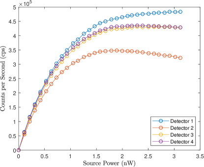
Figure 5: (Color online) In-situ data displaying detector count rate dependence on source power. Signs of detector saturation are visible throughout the dynamic range of the detectors, but dominate at source powers over 2 nW.

A measured laser power level of 1.9 $\mu$W before attenuation through the NDF stack (and 2 nW after attenuation) induced the onset of detector saturation, as shown in Fig. 5. As such, we chose to take measurements at 21 different power levels, in equal increments from 2 nW down to levels near the noise floor or dark-count regime. The dark count regime measurements were taken with no change in the optical setup except closing the in-line fiber attenuator such that the counts registered the minimum values in each detector. Care was taken to measure the dark counts with the fibers connected to the setup as to include any thermal radiation persisting in the fiber.

Data was captured at each power level over a time of about 0.5 s, with 2-ns timing resolution. The time tagger gate time was set to 2 ms in the S-fifteen software, which was chosen in order to prevent overflow of the 16 kB memory register and the 32-bit timestamp index at power levels sufficiently large to induce detector saturation.

IV Analysis Procedure

Output from the timing electronics, which consisted of a list of detection timestamps and the associated detector triggering pattern, was processed using a script capable of designating a specific coincidence window. We used a fixed time segment scheme to organize separate coincident window periods and aggregate multiphoton detections in a similar way to the method used in typical PNR detectors to aggregate counts using a gate or pulsed source. (Another possible method of aggregating multiphoton detections, which we did not use, involves defining coincidence windows relative to individual detections, which is the method that intensity interferometers use to aggregate signals in order to measure $g^{(2)}$ correlations.) In our case, a fixed software-defined coincidence window schedule is more appropriate for comparison against other PNR detectors, is easier to implement, and avoids issues of repeatedly counting particular detections when grouped among different relatively defined coincidence windows (i.e., overlapping coincidence windows). Moreover, a fixed coincidence schedule is among the coincidence counting schemes that evade the coincidence window loophole for Bell tests [64].

An additional complication, common to each method of aggregating multiphoton counts, is that the detector may reset and register a second detection before the governing coincidence window has expired. This situation arises when the chosen coincidence window is a large fraction of the detector dead time for free-running SPDs. This problem is not typically seen in most PNR detectors due to the fact that their effective coincidence window tends to be much smaller than the detector dead time. Source pulsing or detector gating would circumvent this complication [69]; however, this was not possible using our setup, as the pulse rise time for our laser source is rather slow (about 5 $\mu$s) and our detectors do not have hardware gating capability. We avoid this issue in software by forbidding all duplicate detections from the same detector within a coincidence window. A finite detector dead time also engenders a corresponding complication wherein a possible photon could impinge upon the detector while the detector is in a recovery state. This complication is common to all PNR detectors, presumably manifesting as a drop in detector efficiency, and can be mitigated only by improving the detector dead time.

The script we developed aggregates the multi-detector events, which are typically interpreted as multiphoton events. An output file specifies the quantities registered for each associated detector combination, which is then fed into another script that processes the multi-detector counts (i.e., click statistics) using a modified binomial detector model based on work by Sperling, Vogel, and Agarwal (SVA) [70, 71]. The binomial model we used to convert click statistics to photon statistics was expanded to permit individualized detector efficiencies and dark counts, and an unbalanced source distribution across beam splitter paths. This model was developed for coherent sources and as such is relevant for our laser-based system.

According to the model, the probability for $k$ clicks is

$$P_{k}=\sum_{|\boldsymbol{m}|=k}\prod_{i=1}^{N}p_{i}^{m_{i}}\prod_{j=1}^{N}(1-p_{j})^{1-m_{j}}\;.$$ (2)

where $m_{i}\in\{0,1\}$, $|\boldsymbol{m}|=m_{1}+\cdots+m_{N}$, and $p_{i}$ of a detection of the $i^{\rm th}$ detector. For coherent light, and including detector-specific parameters, $p_{i}$ is given by

$$p_{i}=1-e^{-\eta_{i}|u_{i}\alpha|^{2}-\nu_{i}}\;,$$ (3)

where $\eta_{i}$ is the detector efficiency, $1-e^{-\nu_{i}}$ is the probability of a dark count, and $u_{i}\alpha$ is the amplitude of coherent light entering the detector. For a uniform beam splitter network, $u_{i}=1/\sqrt{N}$.

Nominal initial values for detector efficiencies, dark counts, branch weighting, and the click statistics were input to an optimization routine. This routine minimizes a chi-squared metric tracking the overall deviation between the model’s binomial photon distribution and the experimental detector click statistics. For each power level and each coincidence window, the optimization routine was applied to estimate, not only the aforementioned efficiencies, dark counts, and branch weighting, but also the mean photon number, $\mu$. In this way, we could determine the dependence of the mean photon number on both the coincidence window and source power level.

In addition to the experimental data produced, we also developed a script that generates detection events according to a classical model with a stochastic vacuum field component combined with deterministic amplitude-threshold detectors [72, 73]. The classical nature of the model was an intentional feature used to test the possibility of reproducing what is typically interpreted as evidence for the particle nature of light via PNR detectors under purely continuous electromagnetic field conditions. One could construe this test as an exhibition of the suitability of purely classical approaches for interpreting experimental PNR detector results.

Under this model, coherent light is represented as a complex Gaussian random vector with a nonzero mean. Specifically, a coherent state $\ket{\alpha}_{H}\otimes\ket{0}_{V}$ corresponding to a single spatial mode and two orthogonal polarization modes (horizontal and vertical, respectively) may be represented by the random variables

$$a_{H} =\alpha+\sigma z_{H}$$ (4a)

$$a_{V} =\sigma z_{V}\;,$$ (4b)

where $\sigma=1/\sqrt{2}$ is the standard deviation due to the vacuum state and $z_{H},z_{V}$ are independent standard complex Gaussian random variables. So $\mathsf{E}[|a_{H}|^{2}]-\sigma^{2}=|\alpha|^{2}$ corresponds to the average photon number in the horizontal polarization mode, excluding the vacuum contribution.

For a beam splitter network with $N$ output spatial modes, we now have

$$a_{iH} =u_{i}\alpha+\sigma z_{iH}$$ (5a)

$$a_{iV} =\sigma z_{iV}$$ (5b)

where $u_{i}$ is defined as before and $z_{iH},z_{jV}$ are independent standard complex Gaussian random variables.

We treat detections as simple amplitude-threshold-crossing events, so a detection on the $i^{\rm th}$ detector is modeled as the event

$$D_{i}=\{|a_{iH}|>\gamma\;\text{or}\;|a_{iV}|>\gamma\}\;.$$ (6)

It is now straightforward to compute the probabilities for various multidetection events, since all detection events are mutually independent. The probability of exactly $k$ detections will be given by Eqn. (2), with $p_{i}$ replaced by the probability of event $D_{i}$.

V Results

Output from the optimization routine included estimates for the average photon number, detector efficiencies, binomial distribution, and the corresponding Poisson distribution. The click statistics, binomial distribution, and the corresponding Poisson distribution are plotted in Fig. 6 for a source power of 0.11 nW and a 3.5 $\mu$s coincidence window resulting in an average photon number of 2.46. Due to the binary nature of the detectors,[74, 75, 76, 77, 78] which signal either the presence or absence of photons, if one were to ascribe to each detection a single captured photon then many photons would likely be undercounted, as multiple photons may impact a single detector. Using this naïve approach one would expect a Poisson distribution made manifest in the click statistics directly when the detector system is illuminated by a coherent source. However, the Poissonian estimation is valid only for extremely low light levels, where the probability of observing a multiphoton state is negligible. The correct scheme for analyzing arrays of on-off photon detectors is based on the binomial distribution [70, 71].

Instead of using the naïve approach, the Poisson distribution in Fig. 6 was calculated using the average photon number estimated from the optimized binomial distribution. As such, the Poisson distribution probability weighting is shifted toward higher photon numbers, indicating the veiled undercounting of photons due to multiphoton states producing lower order detector click patterns. In this way, the Poisson distribution is reconstructed appearing as if single-photon detectors could count multiple photons. Notably, all probability in the calculated Poisson distribution above a photon number of four is added in the “4+” bin, as this PNR system possessed a maximum photon resolution of four corresponding to the number of detectors. All things considered, Fig. 6 shows both the agreement between click statistics and the fitted binomial distribution as well as the unsuitability of estimating the photon distribution by fitting a Poisson distribution directly to the click statistics.

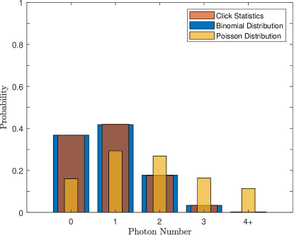
Figure 6: (Color online) Distributions describing photon statistics gathered experimentally for a nominal power of 0.11 nW and coincidence window of 3.5 $\mu$s. Click statistics, integrated over 0.6 seconds, are shown in brown. The fitted binomial distribution is in blue, and the corresponding Poisson distribution, calculated using the binomial model’s average photon number of 2.46, is in gold. The “4+” bin aggregates the probabilities for four or more photons.

As noted previously, we swept through values of both coincidence window as well as source power. Fig. 7 (top panel) shows the click statistics for all values of coincidence window at a source power level of 0.53 nW, and Fig. 7 (bottom panel) illustrates the corresponding binomial distribution resultant from the modified SVA model. We observe, in both cases, the weight of the probability shifting from low photon numbers to higher photon numbers as the coincidence window increases. The discrepancy between the click statistics and the binomial distribution resulted in an average uncertainty below $\pm 1.5\%$ showing excellent agreement.

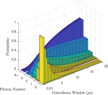
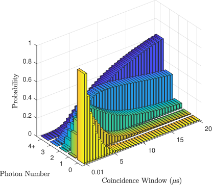
Figure 7: (Color online) Top panel: Click statistics at 0.53 nW. Bottom panel: Binomial distribution at 0.53 nW

Each binomial photon distribution contained an associated average photon number which is plotted in Fig. 8 (top panel) as a function of both coincidence window and source power level. We can see that, as expected, as the source power increases the average photon number increases. We can also observe the normal saturating effect as the source power induces detection rates on par with the dead time of the detector (1 $\mu$s) shown in appendix 1. In addition to these expected characteristics, the average photon number behavior also shows a strong dependence on the coincidence window. To our knowledge no other experimental groups have displayed data showing systematic dependence of calculated photon distribution on coincidence window. The coincidence window dependence, similar to the power dependence, shows some saturating behavior. It must be noted, however, that as the average photon number grows above 4 the certainty with which we may treat the photon distribution diminishes and consequently the validity of the average photon number begins to rely more heavily on the adherence of the laser’s character as representing a true Poissonian light source.

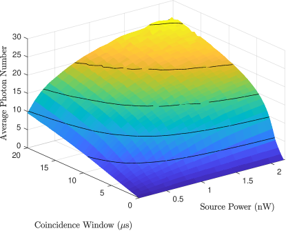
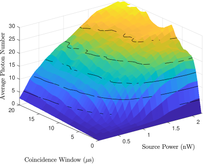
Figure 8: (Color online) Top panel: Average photon number dependence on coincidence window and source power. Data was captured experimentally and passed through an analytical model based on SVA’s work. Bottom panel: Average photon number dependence on coincidence window and source power. Calculated using fully classically modeled detection events, then passed through the SVA binomial model for photon detection.

In addition to gathering experimental data, we also chose to implement a fully classical model based on stochastic vacuum fluctuations and amplitude threshold detection, as described by Eqns. (5) and (6), in order to test if it is possible to replicate the output of a photon number resolving detector without relying on the a priori assumption of light particles. Figure 8 (bottom panel) shows the results of this modeling effort in a one-to-one comparison manner with the experimental results. Indeed, the average photon number constructed purely from the results of the classical model processed in the exact manner as the experimental data shows striking similarity. First, we note the overall similar values on an order of magnitude scale, which we emphasize was not guaranteed as the generally accepted mechanism of operation of PNR detectors, i.e. photon absorption, is not invoked in the simple one-factor model. Secondly, we see similar qualitative behavior at comparable values both in the coincidence window timescale as well as the power level. In particular we observe the relatively rapid rise and gradual saturation of average photon number values as each independent variable increases. As for discrepancies, the model data shows more fine-grained variability even after one application of nearest neighbor averaging, which may be attributed to the slightly shorter overall integration time of the model data. The experimental integration time amounted to 200-300 cycles of 2 ms time periods providing a total of about half a second of total integration time for each combination of coincidence window and power level. Likewise, the model data was integrated over 100 periods of 2 ms, which corresponded to similar 10 MB file sizes for experimental data and model data. The file size limit was necessary for prompt processing of the coincidence window script on a PC i.e. 10 hours total for each model and experiment over all coincidence window and input power combinations. Incidentally, the binomial model optimization script required 11 hours total for each.

VI Discussion

The previous SNR analysis by Malvimat et al. describes the case for incoherent light, as distant starlight has been the principal target of intensity interferometry. In our case, where the light source is a coherent source, Glauber states that “fully coherent fields and delayed coincidence counting measurements carried out in them will reveal no photon correlations at all.” [79] i.e. $g^{(N)}=1$. As a result, in measuring $g^{(N)}$ for coherent sources, we can expect the counting rate of $N$-fold coincidences to be,

$$r_{c}^{(N)}=r_{1}\cdots r_{N}(\Delta t)^{N-1}\,g^{(N)}$$ (7)

where $r_{c}^{(N)}$ is the coincidence rate and $r_{i}$ is the counting rate of the i^th detector. Therefore the coincidence rate, and thus the SNR, will decrease in the same manner as Eqn. 1 due to their similar scaling $\sim(r\Delta t)^{N}$. In this way, results from SNR analysis still hold validity for the coherent light used in our experiment.

In past work, the connection between PNR detectors and higher order correlations has been hinted at partially [80, 81, 82], but the specific relations linking higher order correlations with multiphoton detections as analyzed in this work have not been addressed. Further extending the richness to our assertion that beamsplitter-based PNR detectors operate on the principals of generalized IIs, we claim that all types of PNR detectors constitute generalized intensity interferometers. In order to support this claim we must consider not only coherence time as playing a critical role, but also coherence area. PNR detectors composed of a grid of single photon detectors as in the case of MPPC’s and SNSPD-based PNR detectors must obey a similar rule as the coherence-time-coincidence-window relation. In order for correlated coincidences to dominate the signal over random coincidences the spatial coherence area of the light source must be larger than the size of the detector array. For a beamsplitter based PNR detector this requirement is alleviated since the coherence area must simply cover a single SPD as opposed to a grid of multiple SPDs. As was the case with coherence time, coherence area is not typically considered in normal characterization of PNR detectors. If the coherence time and coherence area satisfy conditions for an acceptable SNR, we can suppose an equivalence between beamsplitter-based multiplexed PNR designs and array-based PNR detectors. In fact, the characteristic parameters coherence time and area, coincidence window, and the number of detectors need only be corresponding for equivalence to hold. The salient tradeoff concerns the relative budgets for spatial and temporal coherence.

The remaining PNR detector type, so-called monolithic detectors, do not possess a grid of pixels, yet nevertheless have the capability of simultaneously registering more than one detection. Examples of monolithic PNR detectors are VLPCs and TESs. Despite these detector types lacking an arranged grid of SPD pixels, the detectors operate as if they do. The excitation regions (the regions of the device which register a detection and therefore require a recovery time period in the same way as an SPD pixel) of both VLPCs [83] and TESs [30] are around 3 microns. The size of the excitation region allows one to calculate the effective number of pixels a monolithic detector possesses. Due to the physical operation principles of monolithic PNR detectors, they act as if they have pixels which require resetting with the variation that the locations of the effective pixels are not bound to a prescribed grid. Therefore, the operation of each type of PNR detector is largely equivalent, provided each type of detector (BS-multiplexed, pixel-based, and monolithic) is subject to the same conditions with respect to coherence time and coherence area. The performance of each type of detector is differentiated largely on single detector dependent characteristics such as dead time, efficiency, and dark counts which themselves constitute a parametric model to be fitted according to physical device conditions e.g. reverse bias voltage or bias current, etc.

VII Conclusion

In this work, we have recognized a hitherto unacknowledged noise source active in the operation of PNR detectors. The noise source comes in the elusive form of accidental coincident detections, which are liable to be mistaken for correlated coincidences. We discuss the experimental parameters pertinent to establishing sufficient SNR and the importance of the relative values of coherence time and coincidence window. Our survey revealed that many common PNR detectors have insufficient SNRs. The PNR detector developed for this work replicated the prevalent low SNR condition to show that variable coincidence windows can indeed alter reported photon statistics. Under these conditions we were able to establish good agreement between experimental results and a fully classical model based on amplitude threshold detection. It remains to be seen if the classical model is sufficient for high SNR conditions. If shown to be sufficient, it would be possible to attribute the multimodal character of PNR detector output to the nonlinear multiplication processes ubiquitous to PNR detectors (i.e. threshold detection) combined with the aforementioned aggregation principle, rather than presuming the prior presence of a certain number of discrete photons. We posit this interpretation, which reflects the underlying assumptions of the classical model, as an alternative to the one-to-one causal relationship between an incoming photon and a consequent photoelectron, that is, the basis for light quanta.

Concerning Einstein’s bubble paradox, in light of the alternative explanation for the operation of PNR detectors discussed above, we may address aspects of this paradox using a classical description. Consider an SPD pixel-based PNR detector spread on the inside of a sphere with a highly attenuated light source situated at the center. Given each pixel operates on amplitude threshold detection and the average energy output of the source is equal to the input energy of the detector, no light particles need be presumed to avoid a paradox. In fact, given such an attenuated light source, the most likely behavior would be long periods of seeming inactivity punctuated mostly by single detector amplitude crossings caused by the combination of the light source and background noise excursions. Rather than all other detectors being suppressed in order to uphold energy conservation in the light particle picture, the simple and most probable activity occurs. In this way, the preconditioned presumption of light quanta is capable of subtly masking the clarity of such explanations.

As previously mentioned, many physical effects considered to be explained exclusively by a dualistic photon picture have now acquired classical explanations. The use of approaches that consider common, unavoidable nuances of experimental and data analytic techniques such as arbitrary coincidence windows or post selection etc., may enable explanation of fundamental quantum phenomena such as the Born rule[72, 84], quantum eraser,[85] entanglement itself,[86] or various Bell-type inequalities[87, 88, 89] with straightforward intuitable resolutions.[90, 91, 92, 93, 94, 95, 96, 97, 98, 99, 100, 101, 102] Needless to say, possible oversight regarding the foundational interpretations of instrument output can have far-reaching effects not only on aspects of quantum computational advantage and quantum communication security, but also on basic physical effects regarded as exclusively quantum.