Extremum Seeking Tracking
for Derivative-free Distributed Optimization

Abstract

In this paper, we deal with a network of agents that want to cooperatively minimize the sum of local cost functions depending on a common decision variable. We consider the challenging scenario in which objective functions are unknown and agents have only access to local measurements of their local functions. We propose a novel distributed algorithm that combines a recent gradient tracking policy with an extremum-seeking technique to estimate the global descent direction. The joint use of these two techniques results in a distributed optimization scheme that provides arbitrarily accurate solution estimates through the combination of Lyapunov and averaging analysis approaches with consensus theory. We perform numerical simulations in a personalized optimization framework to corroborate the theoretical results.

I Introduction

In recent years, distributed optimization over networks of computing and communicating agents is becoming more and more important, see, e.g., [1, 2, 3] for an overview. Moreover, there has been an increasing interest in scenarios in which agents do not have full knowledge of the objective function. This scenario arises, e.g., when the problem at hand is modeled by leveraging on black-box procedures, or when fast or automatic differentiation techniques are not allowed due to computational limitations, see [4].

Solutions to distributed optimization problems correlated to our context are found in two literature currents: collaborative/distributed extremum seeking and distributed zeroth-order/derivative-free optimization.

As for the distributed extremum seeking methodologies, the first branch of works focuses on a “consensus optimization” setup, addressed also in this paper, in which agents minimize the sum of local cost functions all depending on a common decision variable. In [5], network agents run a dynamic average consensus algorithm with their payoffs as inputs, so that the consensus output tracks the global cost. In [6], a continuous-time distributed extremum-seeking algorithm is designed based on saddle point dynamics and is applied to control energy consumption in smart grids. A proportional-integral extremum-seeking design technique is proposed in [7], while, in [8], the gradient is approximated through a real-time parameter estimation. In [9], authors propose the use of the sliding mode to generate the dither signal at the base of the extremum seeking. More recently, in [10], a distributed stochastic extremum seeking scheme is proposed for a source localization problem, while in [11] an optimization problem is solved in a distributed way by applying a Newton method in which both local gradients and local hessian functions are estimated via extremum seeking. Another branch of literature analyzes distributed extremum-seeking methodologies applied to so-called constraint-coupled optimization problems in which local functions depend on local decision variables which are coupled through a global constraint. In [12], an extremum seeking control, based on classical evolutionary game-theory ideas, is designed to perform distributed real-time resource allocation. The work [13] proposes a distributed continuous-time extremum-seeking scheme using sign-based consensus. In [14], a Lie bracket approximation technique is exploited to implement the extremum-seeking strategy for problems with linear constraints. In [15], resource allocation problems are addressed by an extremum-seeking algorithm which is shown to be semi-globally practically stable.

As for distributed zeroth-order/derivative-free optimization, the main idea consists of the approximation of the local gradients through a finite set of (possibly random) evaluations of the cost functions. Authors in [16] develop a zeroth-order scheme based on a one-point estimator and a gradient tracking policy. The work [17] instead proposes a zeroth-order algorithm based on a two-point estimator with a distributed gradient descent strategy and another one based on an $n$-point estimator with a gradient tracking policy. Authors in [18] propose a continuous-time gradient-free approach emulating a distributed gradient algorithm for which optimal asymptotic convergence is guaranteed. In [19], a sampled version of [18] is proposed. In [20], a continuous-time distributed algorithm based on random gradient-free oracles is proposed for convex optimization problems. In [21], the randomized gradient-free oracles introduced in [20] are used to build a gradient-free distributed algorithm in directed networks. Randomized gradient-free algorithms are used also in [22], where sequential Gaussian smoothing is used for non-smooth distributed convex constrained optimization. In [23], gradient-free optimization is addressed with the additional constraint that each agent can only transmit quantized information. The work in [24] instead develops a “directed-distributed projected pseudo-gradient” descent method for directed graphs. Paper [25] combines the gradient-free strategy of [20] with a saddle-point algorithm. Authors in [26] address an online constrained optimization problem by relying on the Kiefer-Wolfowitz algorithm to approximate the gradients, and [27] combines the estimation of the gradient via a “simultaneous perturbation stochastic approximation” technique with the so-called matrix exponential learning optimization method. In [28], a randomized gradient-free method is combined with a state-of-the-art distributed gradient descent approach for directed networks. In [29], an overview of zeroth-order methods based on a Frank-Wolfe framework is provided. Authors in [30] propose a distributed random gradient-free protocol to solve constrained optimization problems by using projection techniques. All the cited papers but [27] prove the stability of the proposed algorithms by using arguments not based on Lyapunov functions. It is worth noting that [27] proposes an algorithm neither based on gradient tracking nor using extremum-seeking approximations.

This paper proposes a novel algorithm to solve a distributed optimization problem in which network agents can only evaluate their local cost function at a given point, but not its gradient. The proposed solution consists of a distributed protocol in which the (unavailable) local gradients are approximated through an extremum seeking scheme. The approximations of the gradients are used to feed a suitable tracking mechanism which, in turn, allows for steering the local solution estimates along approximations of the global descent direction. Moreover, the distributed algorithm uses a further consensus action on the local solution estimates. The convergence of our scheme is proved through Lyapunov and averaging theories for discrete-time systems. It is worth mentioning that our scheme, together with the ones in [31, 32], is the only distributed extremum-seeking scheme proposed in discrete-time with the following distinctive features. The work [31] (i) does not address a consensus optimization problem and (ii) relies on consensus dynamics estimating the global cost, while ours estimates the global gradient. Instead, in [32], (i) the addressed consensus optimization problems have scalar decision variables and (ii) an extremum-seeking technique is combined with a distributed gradient algorithm, i.e., without a tracking mechanism. As for the literature on distributed zeroth-order/derivative-free methods, the closest work is [16] in which extremum seeking is not used and the global gradient is approximated by using a randomized one-point policy. Moreover, our set of Lyapunov-based tools combined with averaging theory for discrete-time systems represent a distinctive feature in the algorithm analysis.

The paper unfolds as follows. Section II introduces the problem and the proposed algorithm. The main result is provided in Section III and proved in Section IV. In Section V, we perform some numerical simulations to show the effectiveness of the proposed algorithm.

Notation

Given $N\in\mathbb{N}$ vectors $x_{1},\dots,x_{N}\in\mathbb{R}^{n}$, we denote by $\mathtt{col}(x_{1},\dots,x_{N})$ their column stacking. Given $N\in\mathbb{N}$ scalars $d_{1},\dots,d_{N}$, we denote by $\mathtt{diag}(d_{1},\dots,d_{N})$ the diagonal matrix with $i$-th entry $d_{i}$. The Kronecker product is denoted by $\otimes$. The identity matrix in ${\mathbb{R}}^{n\times n}$ is $I_{n}$. The column vector of $N\in\mathbb{N}$ ones is denoted by $1_{N}$ and we define $\mathbf{1}:=1_{N}\otimes I_{n}$. Dimensions are omitted whenever they are clear from the context. Finally, for $r>0$, we let $\mathcal{B}_{r}=\{x\in{\mathbb{R}}^{n}\,:\,\left\|x\right\|\leq r\}$.

II Problem Formulation and Gradient Tracking algorithm

We consider a network of $N$ agents communicating according to an undirected graph $\mathcal{G}=(\mathcal{V},\mathcal{E},\mathcal{A})$, where $\mathcal{V}=\{1,\dots,N\}$ is the set of agents, $\mathcal{E}\subseteq\mathcal{V}\times\mathcal{V}$ is the set of edges and $\mathcal{A}=[a_{ij}]\in{\mathbb{R}}^{N\times N}$ is the weighted adjacency matrix. Agent $i$ and $j$ can exchange information only if $(i,j)\in\mathcal{E}$. Accordingly, it holds $a_{ij}\geq 0$ if $(i,j)\in\mathcal{E}$ and $a_{ij}=0$ otherwise. We denote as $\mathcal{N}_{i}=\{j\in\mathcal{V}\mid(i,j)\in\mathcal{E}\}$ the set of neighbors of agent $i$. Moreover, we also associate to the graph the Laplacian matrix $\mathcal{L}:=\mathcal{D}-\mathcal{A}\in{\mathbb{R}}^{N\times N}$, where $\mathcal{D}:=\mathtt{diag}(\mathtt{deg}_{1},\dots,\mathtt{deg}_{N})\in{\mathbb{R}}^{N\times N}$ is the so-called degree matrix in which $\mathtt{deg}_{i}:=\sum_{j\in\mathcal{N}_{i}}a_{ij}$ is the degree of agent $i$. In the rest of the paper, we will use the following assumption on the network communication graph.

Assumption 1

The graph $\mathcal{G}$ is connected and the adjacency matrix $\mathcal{A}\in^{N\times N}$ is symmetric. $\square$

In the proposed distributed setup, each agent $i$ is equipped with a sensor only providing measurements of the local cost function $f_{i}:{\mathbb{R}}^{n}\to{\mathbb{R}}$ and aims at solving the problem

$$\min_{w\in\mathbb{R}^{n}}\sum_{i=1}^{N}f_{i}(w).$$ (1)

We enforce the following assumptions about the problem.

Assumption 2

For all $i\in\{1,\ldots,N\}$, the function $f_{i}$ is $\underline{L}$-strongly convex for some $\underline{L}>0$. $\square$

Assumption 3

Each function $f_{i}$ is (at least) $\mathcal{C}^{3}$ and has $\overline{L}_{i}$-Lipschitz continuous gradients, namely there exists a constant $\overline{L}_{i}>0$ such that for all $i\in\{1,\dots,N\}$ it holds

$$\left\|\nabla f_{i}(x_{1})-\nabla f_{i}(x_{2})\right\|\leq\overline{L}_{i}\left\|x_{1}-x_{2}\right\|,$$

for all $x_{1}$, $x_{2}\in\mathbb{R}^{n}$. We denote $\overline{L}=\max\{\overline{L}_{1},\dots,\overline{L}_{N}\}$. $\square$

Remark 1

Assumption 2 ensures the existence of a unique global minimum $x^{\star}\in\mathbb{R}^{n}$. Moreover, being problem (1) unconstrained, it holds $\sum\limits_{i=1}^{N}\nabla f_{i}(x^{\star})=0$. $\square$

Our aim is to iteratively solve problem (1) via a distributed algorithm. Namely, given the iteration index $t\in\mathbb{N}$ and by denoting with $w_{i}^{t}\in{\mathbb{R}}^{n}$ the $i$-th agent’s estimate, at iteration $t$, of the solution to problem (1), our goal is to design a distributed protocol able to steer all these estimates to the minimizer $x^{\star}$. The peculiar challenge of this paper is that each agent $i$ can access neither the gradients $\nabla f_{i}(w_{i}^{t})$ (as in standard gradient-based methods) nor the cost functions in arbitrary points (as in standard zeroth-order methods). More in detail, we assume that agent $i$ can estimate the local gradient by only using the single measurement $f_{i}(w_{i}^{t})$ properly combined with the so-called dither signal $d_{i}^{t}\in{\mathbb{R}}^{n}$ and the amplitude parameter $\delta>0$. The role of $d_{i}^{t}$ and $\delta$ will become clearer in the next section.

III Extremum Seeking Tracking:
Algorithm Introduction and Convergence

Since the cost gradients are not available, we replace them with an estimation based on a proper elaboration of the local cost function values excited via suitable dithering signals $d_{i}^{t}$. The proposed distributed method, termed Extremum Seeking Tracking, is described in Algorithm 1, from the perspective of agent $i$.

initialization: $x_{i}^{0}\in\mathbb{R}^{n}$ and $z_{i}^{0}=0$

for $t=0,1,\dots$ do

     

$$w_{i}^{t+1} =w_{i}^{t}-\gamma\sum_{j\in\mathcal{N}_{i}}\!\!{\ell}_{ij}(w_{j}^{t}-\delta d_{j}^{t})-\gamma s_{i}^{t}+\delta(d_{i}^{t+1}-d_{i}^{t})$$ (2a)

$$s_{i}^{t+1} =s_{i}^{t}-\!\gamma\!\sum_{j\in\mathcal{N}_{i}}\ell_{ij}s_{j}^{t}+\frac{2}{\delta}(f_{i}(w_{i}^{t+1})d_{i}^{t+1}-f_{i}(w_{i}^{t})d_{i}^{t})\!$$ (2b)

end for

Algorithm 1 Extremum Seeking Tracking (agent $i$)

In Algorithm 1, the parameter $\delta>0$ represents the amplitude of the dither signal $d_{i}^{t}$, while $\gamma>0$ represents the stepsize. The dithering signal $d_{i}^{t}$ is defined as

$$d_{i}^{t}=\mathtt{col}\left(\sin\left(\dfrac{2\pi t}{\tau_{i_{1}}}+\phi_{i_{1}}\right),\,\dots,\,\sin\left(\dfrac{2\pi t}{\tau_{i_{n}}}+\phi_{i_{n}}\right)\right),$$ (3)

where $\tau_{i_{p}}\in\mathbb{N}$ and $\phi_{i_{p}}\in\mathbb{R}$ such that, given $p,q,r\in\{1,\ldots,n\}$, $p\neq q$, $q\neq r$, $p\neq r$, it holds

$$\sum_{t=0}^{\tau_{\text{per}}-1}\sin\left(\tfrac{2\pi t}{\tau_{i_{p}}}+\phi_{i_{p}}\right)\!=\!0$$ (4a)

$$\sum_{t=0}^{\tau_{\text{per}}-1}\sin\left(\tfrac{2\pi t}{\tau_{i_{p}}}+\phi_{i_{p}}\right)\sin\left(\tfrac{2\pi t}{\tau_{i_{q}}}+\phi_{i_{q}}\right)\!=\!\dfrac{\tau_{\text{per}}}{2}$$ (4b)

$$\sum_{t=0}^{\tau_{\text{per}}-1}\sin\!\left(\tfrac{2\pi t}{\tau_{i_{p}}}\!+\!\phi_{i_{p}}\right)\!\sin\!\left(\tfrac{2\pi t}{\tau_{i_{p}}}\!+\!\phi_{i_{p}}\right)\!\sin\!\left(\tfrac{2\pi t}{\tau_{i_{r}}}\!+\!\phi_{i_{r}}\right)\!=\!0,$$ (4c)

for $i\in\{1,\ldots,N\}$. Here, $\tau_{\text{per}}\in\mathbb{N}$ is the least common multiple of all periods $\tau_{ip}$.

The local gradient estimates generated by $\frac{f_{i}(w_{i}^{t})d_{i}^{t}}{2\delta}$ are suitably interlaced with (i) the term $\sum_{j\in\mathcal{N}_{i}}{\ell}_{ij}(w_{j}^{t}-\delta d_{j}^{t})$ to force consensus among the local quantities $w_{i}^{t}-\delta d_{i}^{t}$ and (ii) a tracking mechanism to reconstruct the (estimated) global gradient. More in detail, the consensus step is performed by using the entries $\ell_{ij}$ the $(i,j)$-entry of the Laplacian matrix $\mathcal{L}$ associated to the graph $\mathcal{G}$, while the tracking mechanism is implemented by equipping each agent $i$ with an auxiliary variable $s_{i}^{t}\in{\mathbb{R}}^{n}$. In this algorithm, agents exchange with their neighbors the information $\mathtt{col}(w_{i}^{t}-\delta d_{i}^{t},s_{i}^{t})$ involving $2n$ components.

The convergence properties of Extremum Seeking Tracking are formalized in the next theorem.

Theorem 1

Consider (2) and let Assumptions 1, 2, and 3 hold. Then, for any $r,\bar{\rho}>0$, there exist $\gamma^{\star},\delta^{\star},k_{1}>0$, $\epsilon\in(0,\bar{\rho}/2)$, and $k_{2}\geq(\bar{\rho}/2-\epsilon)$ such that, for any $\gamma\in(0,\gamma^{\star})$, $\mathtt{col}(w_{i},s_{i})\in\mathcal{D}_{i}:=\{\mathtt{col}(w_{i}^{0},z_{i}^{0})\in{\mathbb{R}}^{2n}\mid\left\|w_{i}-x^{\star}\right\|\leq r,s_{i}=\frac{2f_{i}(w_{i}^{0})}{\delta_{i}}\}$, $\delta\in(0,\delta^{\star})$, $i\in\{1,\ldots,N\}$, the trajectories of (2) are bounded and for each $i\in\{1,\ldots,N\}$

$$\left\|w_{i}^{t}-x^{\star}\right\|\leq\bar{\rho},$$ (5)

for all $t\geq t^{\star}$, where $t^{\star}\!:=\!-\frac{1}{\gamma k_{1}}\ln((\bar{\rho}/2\!-\!\epsilon)/k_{2})$, i.e., the convergence to the set $\{w_{i}\in{\mathbb{R}}^{n}\mid\left\|w_{i}^{t}\!-\!x^{\star}\right\|\leq\bar{\rho}\}$ is linear. $\square$

The proof of Theorem 1 is provided in Section IV-C. It is worth noting that Theorem 1 provides a semi-global, practical exponential-stability result restricted to the set $\mathcal{D}:=\mathcal{D}_{1}\times\dots\times\mathcal{D}_{N}$. Indeed, it is semi-global because the parameters $\gamma^{\star}$ and $\delta^{\star}$ depend on the initial radius $r$ and it is practical because they also depend on the arbitrary small final radius $\bar{\rho}>0$.

IV Extremum Seeking Tracking:
Stability Analysis

In this section, we give the convergence proof of Extremum Seeking Tracking. Assumptions 1, 2, and 3 hold throughout the whole section. We first introduce the novel coordinates $x_{i}^{t},z_{i}^{t}\in{\mathbb{R}}^{n}$ defined as

$$x_{i}^{t}:=w_{i}^{t}-\delta d_{i}^{t},\quad z_{i}^{t}:=s_{i}^{t}-\frac{2f_{i}(w_{i}^{t})d_{i}^{t}}{\delta},$$ (6)

for all $i\in\{1,\ldots,N\}$, which allow us to rewrite (2) as

$$x_{i}^{t+1} =x_{i}^{t}\!-\!\gamma\!\left(\sum_{j\in\mathcal{N}_{i}}\!\!{\ell}_{ij}x_{j}^{t}+z_{i}^{t}+\frac{2f_{i}(x_{i}^{t}+\delta d_{i}^{t})d_{i}^{t}}{\delta}\!\right)$$ (7a)

$$z_{i}^{t+1} =z_{i}^{t}\!-\!\gamma\!\sum_{j\in\mathcal{N}_{i}}\ell_{ij}\left(z_{j}^{t}+\frac{2f_{j}(x_{j}^{t}+\delta d_{j}^{t})d_{j}^{t}}{\delta}\right).$$ (7b)

Remark 2

In the case of a perfect gradient estimation, the distributed algorithm (7) would read as

$$x_{i}^{t+1} ={x_{i}^{t}}-{\gamma}\sum_{j\in\mathcal{N}_{i}}{\ell}_{ij}x_{j}^{t}-\gamma\left(z_{i}^{t}+\nabla f_{i}(x_{i}^{t})\right)$$ (8a)

$$z_{i}^{t+1} ={z_{i}^{t}}-{\gamma}\sum_{j\in\mathcal{N}_{i}}{\ell}_{ij}\left(z_{j}^{t}+\nabla f_{j}(x_{j}^{t})\right).$$ (8b)

It is worth noting that it is possible to interpret (8) as the discrete-time version of the continuous-time gradient tracking proposed in [33]. The analysis required to prove Theorem 1 will also require the investigation of the convergence properties of (8) (see Lemma 3 and Remark 4). $\square$

Then, we aggregate the local updates in (7) obtaining the compact algorithm description

$${x}^{t+1} =\,x^{t}-\gamma\left(L{x}^{t}+z^{t}+f_{d}(t,x^{t})\right)$$ (9a)

$${z}^{t+1} =\,z^{t}-\gamma\left(L{z}^{t}+Lf_{d}(t,x^{t})\right),$$ (9b)

where we introduced $L:=\mathcal{L}\otimes I_{n}$, $x^{t}:=\mathtt{col}(x_{1}^{t},\dots,x_{N}^{t})$, $z^{t}:=\mathtt{col}(z_{1}^{t},\dots,z_{N}^{t})$, $d^{t}:=\mathtt{col}(d_{1}^{t},\dots,d_{N}^{t})$, $\delta:=\mathtt{diag}(I_{n},\dots,I_{n})\otimes I_{n}$, and the function $f_{d}:\mathbb{N}\times{\mathbb{R}}^{Nn}\to{\mathbb{R}}^{Nn}$ defined as

$$f_{d}(t,x):=\begin{bmatrix}2f_{1}(x_{1}+\delta_{1}d_{1}^{t})d_{1}^{t}/\delta_{1}\\ \vdots\\ 2f_{N}(x_{N}+\delta_{N}d_{N}^{t})d_{N}/\delta_{N}\end{bmatrix},$$ (10)

where we decomposed $x$ according to $x:=\mathtt{col}(x_{1},\dots,x_{N})$ with $x_{i}\in{\mathbb{R}}^{n}$ for all $i\in\{1,\ldots,N\}$. We point out that, see also Fig. 1, system (9) can be conceived as an extremum-seeking scheme with output map $f(x+\delta d^{t})$.

Figure 1: Block scheme of the proposed Extremum Seeking Tracking algorithm in the $(x,z)$ coordinates.

We now give an overview of the main steps of the stability analysis carried out to prove Theorem 1:

1. We perform a first change of variables to describe the dynamics (9) in terms of the mean value (over the agents) $\tilde{z}_{\text{avg}}$ of $z$ and the orthogonal part $\tilde{z}_{\perp}$ associated to the consensus error. Then, by relying on averaging theory (see [34] for discrete-time systems or [35, Ch.10] and [36] for continuous-time systems), we introduce a suitable auxiliary system named averaged system. The latter is obtained by averaging the original algorithm dynamics over a common period. The averaged system is shown to be driven by the local function gradients with additive estimation errors.

2. When neglecting these errors, the averaged system corresponds to an equivalent form of (8). Based on this observation, we rely on existing stability properties of the continuous gradient tracking to demonstrate that the trajectories of the averaged system exponentially converge to an arbitrarily small neighborhood of $\mathtt{col}(\mathbf{1}x^{\star},\tilde{z}^{\text{eq}}_{\perp})$ for some $\tilde{z}^{\text{eq}}_{\perp}$ arising from the analysis.

3. Finally, we prove Theorem 1 by exploiting the steps above and by using averaging theory to show the closeness between the trajectories of (9) and those of its averaged system.

Step (i) is performed in Section IV-A, while step (ii) is carried out in Section IV-B. Section IV-C is devoted to the development of step (iii).

IV-A Coordinate changes and averaged system

We start by introducing a change of coordinates to highlight the error dynamics. To this end, let us introduce $G:{\mathbb{R}}^{Nn}\to{\mathbb{R}}^{Nn}$ be defined as

$$G(x):= \,\mathtt{col}(\nabla f_{1}(x_{1}),\dots,\nabla f_{N}(x_{N})).$$ (11)

Then, let the error coordinates $\tilde{x},\tilde{z}\in{\mathbb{R}}^{Nn}$ be

$$\tilde{x}:=x-\mathbf{1}x^{\star},\quad\tilde{z}=z+G(\mathbf{1}x^{\star}),$$ (12)

and let us introduce $\phi_{xz}:\mathbb{N}\times{\mathbb{R}}^{Nn}\times{\mathbb{R}}^{Nn}\to{\mathbb{R}}^{2Nn}$ as

$$\phi_{xz}(t,\tilde{x},\tilde{z})\!\!:=\!\!\begin{bmatrix}-L\tilde{x}-\tilde{z}-f_{d}(t,\tilde{x}+\mathbf{1}x^{\star})+G(\mathbf{1}x^{\star})\\ -L\tilde{z}-L(f_{d}(t,\tilde{x}+\mathbf{1}x^{\star})+G(\mathbf{1}x^{\star}))\end{bmatrix}\!,$$

Then, by using the new coordinates, we rewrite (9) as

$$\begin{bmatrix}\tilde{x}^{t+1}\\ \tilde{z}^{t+1}\end{bmatrix}=\begin{bmatrix}\tilde{x}^{t}\\ \tilde{z}^{t}\end{bmatrix}+\gamma\phi_{xz}(t,\tilde{x}^{t},\tilde{z}^{t}),$$ (13)

where we have used the property $L\mathbf{1}=0$. Let $n_{\xi}:=(2N-1)n$. As in [33], we take advantage of the initialization $z_{i}^{0}=0$ for all $i\in\{1,\ldots,N\}$ by introducing the novel coordinates $z_{\text{m}}\in{\mathbb{R}}^{n}$, $\tilde{z}_{\perp}\in{\mathbb{R}}^{(N-1)n}$, and $\xi\in{\mathbb{R}}^{n_{\xi}}$ defined as

$$\begin{bmatrix}\tilde{z}_{\text{m}}\\ \tilde{z}_{\perp}\end{bmatrix}:=\begin{bmatrix}\frac{\mathbf{1}^{\top}}{N}\\ R^{\top}\end{bmatrix}\tilde{z},\quad\xi:=\begin{bmatrix}\tilde{x}\\ \tilde{z}_{\perp}\end{bmatrix},$$ (14)

where we introduced the matrix $R\in{\mathbb{R}}^{Nn\times(N-1)n}$ such that $R^{\top}\mathbf{1}=0$, $R^{\top}R=I$. Then, since $\mathbf{1}^{\top}L=0$ in light of Assumption 1 and $\mathbf{1}^{\top}G(\mathbf{1}x^{\star})=\sum_{i=1}^{N}\nabla f_{i}(x^{\star})=0$ (since $x^{\star}$ is the minimizer of problem (1)), system (13) reads as

$$\xi^{t+1} =\xi^{t}+\gamma\phi_{\xi}(t,\mathtt{col}(\tilde{x}^{t},\mathbf{1}\tilde{z}_{\text{m}}^{t}+R\tilde{z}_{\perp}^{t}))$$ (15a)

$$\tilde{z}_{\text{m}}^{t+1} =\tilde{z}_{\text{m}}^{t},$$ (15b)

where we introduced $\phi_{\xi}:\mathbb{N}\times{\mathbb{R}}^{2Nn}\to{\mathbb{R}}^{(2N-1)n}$ defined as

$$\phi_{\xi}(t,\mathtt{col}(\tilde{x},\tilde{z})):=\begin{bmatrix}I&0\\ 0&R\end{bmatrix}\phi_{xz}(t,\tilde{x},\tilde{z}).$$ (16)

The equation (15b) allows us to claim that $\tilde{z}_{\text{m}}^{t}=\tilde{z}_{\text{m}}^{0}$ for all $t\geq 0$. Moreover, we recall that (i) $z_{i}^{0}=0$ for all $i\in\{1,\ldots,N\}$, and (ii) $\mathbf{1}^{\top}G(\mathbf{1}x^{\star})=0$. Hence, it holds $\tilde{z}_{\text{m}}^{0}=0$ which allows us to ignore (15b) and rewrite (15) according to the equivalent, reduced system

$$\xi^{t+1}=\xi^{t}+\gamma\phi(t,\xi^{t}),$$ (17)

where $\phi:\mathbb{N}\times{\mathbb{R}}^{n_{\xi}}\to{\mathbb{R}}^{n_{\xi}}$ is introduced to compactly describe system (15a) with $\tilde{z}_{\text{m}}^{t}=0$ for all $t\geq 0$, i.e., $\phi$ is defined as

$$\phi(t,\xi) :=\phi_{\xi}(t,\underbrace{\mathtt{col}(\tilde{x},R\tilde{z}_{\perp})}_{\xi})$$ (18)

$$\stackrel{{\scriptstyle(a)}}{{=}}\!\begin{bmatrix}I&0\\ 0&R\end{bmatrix}\!\!\begin{bmatrix}-L\tilde{x}-R\tilde{z}_{\perp}-f_{d}(t,\tilde{x}+\mathbf{1}x^{\star})+G(\mathbf{1}x^{\star})\\ -LR\tilde{z}_{\perp}-L(f_{d}(t,\tilde{x}+\mathbf{1}x^{\star})+G(\mathbf{1}x^{\star}))\end{bmatrix}\!\!,$$

where in $(a)$ we used the definition of $\phi_{\xi}$ (cf. (16)).

We resort to the averaging theory [34] to analyze the time-varying system (17). The averaging theory-related investigations introduce an auxiliary scheme typically named averaged system, obtained by averaging the time-varying vector field $\phi(t,\xi)$ over $\tau_{\text{per}}$ samples by freezing the system state. In detail, the averaged system associated with (17) is

$$\xi_{\text{avg}}^{t+1}=\xi_{\text{avg}}^{t}+\gamma\phi_{\text{avg}}(\xi_{\text{avg}}^{t}),\quad\quad\quad\text{(averaged system)}$$ (19)

with $\xi_{\text{avg}}^{0}=\xi_{0}$, where $\phi_{\text{avg}}:{\mathbb{R}}^{n_{\xi}}\to{\mathbb{R}}^{n_{\xi}}$ is defined as

$$\phi_{\text{avg}}(\xi):=\frac{1}{\tau_{\text{per}}}\sum_{k=t+1}^{t+\tau_{\text{per}}}\phi(k,\xi),\quad\text{for any }t\geq 0.$$ (20)

Notice that, since $\phi(k,\xi)$ is periodic with period $\tau_{\text{per}}$ on the first argument, the function $\phi_{\text{avg}}(\xi)$ (cf. (20)) is time-invariant.

The next lemma shows that the gradient of each $f_{i}$ can be approximated by averaging each block of $f_{d}$ (cf. (10)) over the period $\tau_{\text{per}}$ on the first argument. For this reason, the next lemma will be useful to explicitly write $\phi_{\text{avg}}$ (cf. (20)) in terms of $G(x)$, (i.e., the stack of the gradients $\nabla f_{i}(x_{i})$, see (11)).

Lemma 1 (Gradient estimation)

For all $i\in\{1,\ldots,N\}$, there exists $\ell_{i}:\mathbb{R}^{n}\to\mathbb{R}^{n}$ such that, for any given $x_{i}\in{\mathbb{R}}^{n}$ and all $t\geq 0$, it holds

$$\dfrac{2}{\delta\tau_{\text{per}}}\sum_{k=t+1}^{t+\tau_{\text{per}}}f_{i}(x_{i}+\delta d_{i}^{k})d_{i}^{k}=\nabla f_{i}(x_{i})+\delta^{2}\ell_{i}(x_{i}).$$ (21)

Moreover, given any compact set $\mathcal{S}_{i}\subset{\mathbb{R}}^{n}$, if $\delta\in(0,1]$, there exists $L_{i,\mathcal{S}_{i}}>0$ such that

$$\left\|\ell_{i}(x_{i})\right\|\leq L_{i,\mathcal{S}_{i}},$$ (22)

for all $x_{i}\in\mathcal{S}_{i}$ and $i\in\{1,\ldots,N\}$. $\square$

The proof of Lemma 1 is in Appendix -A.

We note that the quantity on the right-hand side of (21) is time-invariant because $d_{i}^{k}$ is periodic, with period $\tau_{\text{per}}$, and the left-hand side of (21) is averaged over the period $\tau_{\text{per}}$. Now, let us introduce the function $\ell:{\mathbb{R}}^{Nn}\to{\mathbb{R}}^{Nn}$ stacking all the approximation errors $\ell_{i}(x_{i})$ used in (21), namely

$$\ell(x):=\mathtt{col}\left(\ell_{1}(x_{1}),\dots,\ell_{N}(x_{N})\right).$$ (23)

Then, by using (21), the definitions of $f_{d}$ in (10), $G(x)$ as the stack of the gradients $\nabla f_{i}(x_{i})$ in (11), and $\ell(x)$ as the stack of the approximation errors $\ell_{i}(x_{i})$ in (23), it holds

$$\frac{1}{\tau_{\text{per}}}\sum_{k=t+1}^{t+\tau_{\text{per}}}f_{d}(k,x)=G(x)+\ell(x),$$ (24)

for all $x\in{\mathbb{R}}^{Nn}$ and $t\geq 0$. Hence, by introducing $\xi_{\text{avg}}:=\mathtt{col}(\tilde{x}_{\text{avg}},\tilde{z}_{\perp,_{\text{avg}}})$ and by combining the definition of $\phi_{\text{avg}}$ in (20), $\phi$ in (18), and (24), we obtain

$$\phi_{\text{avg}}(\xi_{\text{avg}}) =\begin{bmatrix}-L\tilde{x}_{\text{avg}}-R\tilde{z}_{\perp,_{\text{avg}}}-G(\tilde{x}_{\text{avg}}+\mathbf{1}x^{\star})+G(\mathbf{1}x^{\star})\\ -R^{\top}LR\tilde{z}_{\perp,_{\text{avg}}}-R^{\top}L(G(\tilde{x}+\mathbf{1}x^{\star})-G(\mathbf{1}x^{\star}))\end{bmatrix}$$

$$\hskip 11.38092pt+\begin{bmatrix}-\ell(\tilde{x}_{\text{avg}}+\mathbf{1}x^{\star})\\ -R^{\top}L\ell(\tilde{x}_{\text{avg}}+\mathbf{1}x^{\star})\end{bmatrix}.$$ (25)

We define

$$\phi_{GT}(\xi_{\text{avg}}) :=\begin{bmatrix}-L\tilde{x}_{\text{avg}}-R\tilde{z}_{\perp,_{\text{avg}}}-G(\tilde{x}_{\text{avg}}+\mathbf{1}x^{\star})+G(\mathbf{1}x^{\star})\\ -R^{\top}LR\tilde{z}_{\perp,_{\text{avg}}}-R^{\top}L(G(\tilde{x}+\mathbf{1}x^{\star})-G(\mathbf{1}x^{\star}))\end{bmatrix}$$

$$B :=\begin{bmatrix}-I\\ -R^{\top}L\end{bmatrix}$$

$$M_{\delta} :=\mathtt{diag}(\delta_{1}^{2},\dots,\delta_{N}^{2})\otimes I_{n}$$

$$u(\xi_{\text{avg}}) :=\ell(\tilde{x}_{\text{avg}}+\mathbf{1}x^{\star})$$

to short (25) as

$$\phi_{\text{avg}}(\xi_{\text{avg}})=\phi_{GT}(\xi_{\text{avg}})+BM_{\delta}u(\xi_{\text{avg}}),$$

which, in turn, allows us to rewrite (19) as

$$\xi_{\text{avg}}^{t+1}=\xi_{\text{avg}}^{t}+\gamma\phi_{GT}(\xi_{\text{avg}})+\gamma BM_{\delta}u(\xi_{\text{avg}})\quad\text{(averaged system)}.$$ (26)

Remark 3

It is worth highlighting the main distinctive features of our method. First, the finite differences methods are characterized by estimation errors involving second-order terms of the local cost function expansion, while our estimation policy allows for estimation errors involving third-order terms and, thus, a higher precision. Second, the estimation of the gradients is performed according to a single-point estimator and, thus, the objective functions queries and, possibly, communications are reduced. Also, in some application scenarios, it may be not possible to have multiple samples of the cost function, but the user/agent/robot should decide just one. Third and final, the estimation policy is purely deterministic and, thus, the convergence guarantees are deterministic too. $\square$

IV-B Averaged System Analysis

In this subsection, we analyze the averaged system (26). To this end, we first consider an additional nominal system in which the term $\gamma BM_{\delta}u(\xi_{\text{avg}}^{t})$ (i.e., the term describing the gradients’ estimation error) is neglected. Then, by using such a nominal system analysis as a building block, we provide the result concerning system (26). Therefore, we start by studying

$$\xi_{\text{avg}}^{t+1}=\xi_{\text{avg}}^{t}+\gamma\phi_{GT}(\xi_{\text{avg}}^{t}),$$ (27)

which corresponds to system (26) in the case of $\gamma BM_{\delta}u(\xi_{\text{avg}}^{t})=0$. The next lemma proves the global exponential stability of the origin for (27).

Lemma 2

There exist $P=P^{\top}\in{\mathbb{R}}^{n_{\xi}\times n_{\xi}}$, $a_{1},a_{2},c_{1}>0$, and $\gamma_{0}>0$ such that, for any $\gamma\in(0,\gamma_{0})$, along the trajectories of (27) it holds

$$a_{1}I\leq P \leq a_{2}I$$ (28a)

$${\xi_{\text{avg}}^{t+1}}^{\top}P\xi_{\text{avg}}^{t+1}-{\xi_{\text{avg}}^{t}}^{\top}P\xi_{\text{avg}}^{t} \leq-\gamma c_{1}\left\|\xi_{\text{avg}}^{t}\right\|^{2},$$ (28b)

for all $\xi_{\text{avg}}\in{\mathbb{R}}^{n_{\xi}}$. $\square$

The proof of Lemma 2 is in Appendix -B.

Remark 4

Notice that Lemma 2 proves the algorithm (8) linearly converges to the minimizer of (1), since (27) is an equivalent formulation of (8). $\square$

With this result at hand, we analyze the impact of $u(\cdot)$ thus obtaining the stability properties for the averaged system (26).

Lemma 3

Consider the averaged system (26). Assume that there exist $a_{1},a_{2},c_{1}>0$ and $P=P^{\top}\in{\mathbb{R}}^{n_{\xi}\times n_{\xi}}$ such that conditions (28) hold. Then, for any $r_{\xi}>0,c_{1}^{\prime}\in(0,c_{1})$, and $\rho\in(0,r_{\xi})$, there exist $c_{3}\geq 0$ and $\delta^{\star}_{1}\in(0,1]$ such that, for any $\gamma\in(0,1]$, $\delta\in(0,\delta^{\star}_{1})$, $i\in\{1,\ldots,N\}$, and $\left\|\xi_{\text{avg}}^{0}\right\|\leq r_{\xi}$, it holds
(i) $\xi_{\text{avg}}^{t}\in\mathcal{B}_{\sqrt{a_{2}/a_{1}}r_{\xi}}$ for all $t\geq 0$, and
(ii)

$$\|\xi_{\text{avg}}^{t}\|\leq\sqrt{a_{2}/a_{1}}\exp\left(-t\gamma c_{3}\right)\|\xi_{\text{avg}}^{0}\|,$$ (29)

for all $\left\|\xi_{\text{avg}}^{t}\right\|\geq\rho$. $\square$

The proof of Lemma 3 is in Appendix -C.

Remark 5

The result of Lemma 3 only involves the averaged system (26). In the next section, such a result will be used as a building block to study the original dynamics, i.e., system (17) and, thus, to conclude the proof of Theorem 1. However, it is a per se result that can be used to show robust stability for the distributed algorithm (8).

IV-C Proof of Theorem 1

Despite averaging tools for discrete-time systems are already present in the literature, see [34] for example, we got the inspiration from continuous-time averaging [35, Ch. 10] and [36] for elaborating the proof of Theorem 1 to make clear how $\gamma$ affects the closeness of the trajectories of (17) and (26).

Since Assumptions 1, 2, and 3 hold, we apply Lemma 2 to claim that there exists $P=P^{\top}\in{\mathbb{R}}^{n_{\xi}\times n_{\xi}}$, $\gamma_{0}>0$, and $a_{1},a_{2},c_{1}>0$ such that, if $\gamma\in(0,\gamma_{0})$, the conditions (28) are satisfied. Then, we evaluate the distance with respect to the origin of the initial conditions of system (17) and (26), i.e., $\left\|\xi^{0}\right\|=\left\|\xi^{0}_{\text{avg}}\right\|$. By using the definition of $\xi$, the changes of variables (12) and (14), and the triangle inequality, we get

$$\left\|\xi^{0}\right\| \leq\left\|x^{0}-\mathbf{1}x^{\star}\right\|+\left\|R^{\top}(z^{0}+G(\mathbf{1}x^{\star}))\right\|$$

$$\hskip 11.38092pt+\left\|\frac{\mathbf{1}^{\top}}{N}(z^{0}+G(\mathbf{1}x^{\star}))\right\|\stackrel{{\scriptstyle(a)}}{{\leq}}r\sqrt{N}+\left\|R\right\|\left\|G(\mathbf{1}x^{\star})\right\|,$$

where in $(a)$ we combine the initialization $\left\|x_{i}^{0}-x^{\star}\right\|\leq r$ and $z_{i}^{0}=0$ for all $i\in\{1,\ldots,N\}$ with the fact that $\mathbf{1}^{\top}G(\mathbf{1}x^{\star})=\sum_{i=1}^{N}f_{i}(x^{\star})=0$. Hence, by defining $r_{\xi}:=r\sqrt{N}+\left\|R\right\|\left\|G(\mathbf{1}x^{\star})\right\|$, we claim that

$$\left\|\xi^{0}\right\|=\left\|\xi_{\text{avg}}^{0}\right\|\leq r_{\xi}.$$

Once the initial distance from the origin has been evaluated, we choose any $\bar{\rho}>0$, set $c_{2}:=\sqrt{a_{2}/a_{1}}$, and choose any $\epsilon\in(0,\bar{\rho}(1+c_{2})/2)$. Then, we pick $\rho\in(0,(\bar{\rho}/2-(1+c_{2})\epsilon)/c_{2})$, $c_{1}^{\prime}\in(0,c_{1})$, and use the matrix $P$ satisfying (28) to apply Lemma 3. Specifically, we claim that there exist $c_{3}>0$, and $\delta^{\star}_{1}\in(0,1]$ such that, for any $\delta\in(0,\delta^{\star}_{1})$ for all $i\in\{1,\ldots,N\}$ and $\gamma\in(0,1]$, it holds (i) $\xi_{\text{avg}}^{t}\in\mathcal{B}_{c_{2}r_{\xi}}$ for all $t\geq 0$, and (ii) the inequality $\left\|\xi_{\text{avg}}^{t}\right\|\leq c_{2}\exp(-t\gamma c_{3})\left\|\xi_{\text{avg}}^{0}\right\|$, for all $\xi_{\text{avg}}^{t}$ such that $\left\|\xi_{\text{avg}}^{t}\right\|\geq\rho$. Now, in order to bound $\|\xi^{t}-\xi_{\text{avg}}^{t}\|$, let us introduce

$$\upsilon(t,\xi_{\text{avg}}):=\sum_{k=0}^{t-1}\left(\phi(k,\xi_{\text{avg}})-\phi_{\text{avg}}(\xi_{\text{avg}})\right).$$

By using this definition and the one of $\phi_{\text{avg}}$ (cf. (20)), it holds

$$\upsilon(t+1,\xi_{\text{avg}}^{t+1})-\upsilon(t,\xi_{\text{avg}}^{t})$$

$$=\phi(t,\xi_{\text{avg}}^{t+1})-\phi_{\text{avg}}(\xi_{\text{avg}}^{t+1})+\upsilon(t,\xi_{\text{avg}}^{t+1})-\upsilon(t,\xi_{\text{avg}}^{t}).$$ (30)

Then, let $r_{\xi}^{\prime}:=c_{2}r_{\xi}$ and define $\Delta:=\delta\sqrt{Nn}$. Under the assumption of $\xi^{t}\in\mathcal{B}_{r_{\xi}^{\prime}+\epsilon}$ for all $t\geq 0$ (later verified by a proper selection of $\gamma$), we claim that the arguments of the functions $f_{i}$ and their derivatives (embedded into the definitions of $\phi(t,\cdot)$ and $\phi_{\text{avg}}(\cdot)$ and their derivatives) lie into the compact set $\mathcal{B}_{r^{\prime}_{\xi}+\epsilon+\Delta}$. Thus, since the functions $f_{i}$ and its derivatives are continuous (cf. Assumption 3) and the functions $\phi(\cdot,\cdot)$ and $\nu(\cdot,\cdot)$ are periodic in the first argument, we define

$$L_{\phi}:=\sup_{\begin{subarray}{c}\xi\in\mathcal{B}_{r_{\xi}^{\prime}+\epsilon}\\ t\in[0,\tau_{\text{per}}]\end{subarray}}\bigg{\{} \left\|\phi(t,\xi)\right\|,\left\|\phi_{\text{avg}}(\xi)\right\|,\left\|\frac{\partial\phi(t,\xi)}{\partial\xi}\right\|,$$

$$\left\|\frac{\partial\phi_{\text{avg}}(\xi)}{\partial\xi}\right\|,\left\|\frac{\partial\nu(t,\xi)}{\partial\xi}\right\|\bigg{\}}.$$

Consequently, it holds

$$\|\upsilon(t,\xi)\| \leq 2L_{\phi}\tau_{\text{per}}$$ (31a)

$$\|\phi(t,\xi)-\phi(t,\xi^{\prime})\| \leq L_{\phi}\|\xi-\xi^{\prime}\|$$ (31b)

$$\|\phi_{\text{avg}}(\xi)-\phi_{\text{avg}}(\xi^{\prime})\| \leq L_{\phi}\|\xi-\xi^{\prime}\|$$ (31c)

$$\|\upsilon(t,\xi)-\upsilon(k,\xi^{\prime})\| \leq 2L_{\phi}\tau_{\text{per}}\|\xi-\xi^{\prime}\|$$ (31d)

$$\left\|\phi_{\text{avg}}(\xi)\right\| \leq L_{\phi},$$ (31e)

for all $\xi,\xi^{\prime}\in\mathcal{B}_{r_{\xi}^{\prime}+\epsilon}$ and $t\geq 0$. Let us introduce $\zeta^{t}\in{\mathbb{R}}^{n_{\xi}}$ defined as

$$\zeta^{t}:=\xi_{\text{avg}}^{t}+\gamma\upsilon(t,\xi_{\text{avg}}^{t}).$$

Then, it holds

$$\xi^{t}-\zeta^{t} =\sum_{k=0}^{t-1}(\xi^{k+1}-\xi^{k})-(\zeta^{k+1}-\zeta^{k}),$$

add $\pm\gamma\sum_{k=0}^{t-1}(\phi(k,\zeta^{k})+\phi(k,\xi_{\text{avg}}^{k})),$ and use (30) to get

$$\xi^{t}-\zeta^{t}=\gamma\sum_{k=0}^{t-1}(\phi(k,\xi^{k})-\phi(k,\zeta^{k}))$$

$$+\gamma\sum_{k=0}^{t-1}(\phi(k,\zeta^{k})-\phi(k,\xi_{\text{avg}}^{k}))$$

$$\hskip 11.38092pt-\gamma\sum_{k=0}^{t-1}(\phi(k,\xi_{\text{avg}}^{k+1})-\phi(k,\xi_{\text{avg}}^{k}))$$

$$+\gamma\sum_{k=0}^{t-1}(\phi_{\text{avg}}(\xi_{\text{avg}}^{k+1})-\phi_{\text{avg}}(\xi_{\text{avg}}^{k}))$$

$$\hskip 11.38092pt-\gamma\sum_{k=0}^{t-1}(\upsilon(k,\xi_{\text{avg}}^{k+1})-\upsilon(k,\xi_{\text{avg}}^{k})).$$

Use (17), (26), and (31) to bound

$$\|\xi^{t}-\zeta^{t}\| \leq\gamma L_{\phi}\sum_{k=0}^{t-1}\|\xi^{k}-\zeta^{k}\|+\gamma^{2}L_{\phi}^{2}2\left(1+2\tau_{\text{per}}\right)t.$$

Apply the discrete Gronwall inequality (see [37, 38]) and

$$\sum_{k=0}^{t-1}\gamma L_{\phi}k\exp\left(-\gamma L_{\phi}k\right)\leq\sum_{k=0}^{\infty}\gamma L_{\phi}k\exp\left(-\gamma L_{\phi}k\right)=1$$

to get

$$\|\xi^{t}-\zeta^{t}\|\leq \,\gamma^{2}L_{\phi}^{2}2\left(1+2\tau_{\text{per}}\right)t+\gamma L_{\phi}2\left(1+2\tau_{\text{per}}\right)\exp\left(\gamma L_{\phi}t\right),$$

from which

$$\|\xi^{t}-\xi_{\text{avg}}^{t}\| \leq\gamma^{2}L_{\phi}^{2}2\left(1+2\tau_{\text{per}}\right)t$$

$$\hskip 11.38092pt+\gamma L_{\phi}2\left(1+2\tau_{\text{per}}\right)\exp\left(\gamma L_{\phi}t\right)+\gamma 2L_{\phi}\tau_{\text{per}}.$$

Then, set $\theta^{\star}\in\mathbb{N}$ such that

$$\theta^{\star}\geq-\tfrac{1}{c_{3}}\ln\left(\tfrac{(\bar{\rho}/2-\epsilon)/c_{2}}{c_{2}r_{\xi}}\right).$$ (32)

Let $\gamma_{2}:=\tfrac{\epsilon/3}{L_{\phi}^{2}2\left(1+2\tau_{\text{per}}\right)\theta^{\star}}$, $\gamma_{3}:=\tfrac{\epsilon/3}{2L_{\phi}(1+2\tau_{\text{per}})\exp(L_{\phi}\theta^{\star})}$,$\gamma_{4}:=\tfrac{\epsilon/3}{2L_{\phi}\tau_{\text{per}}}$, $\gamma_{1}:=\min\{\gamma_{2},\gamma_{3},\gamma_{4},1\}$, and $t^{\star}:=\theta^{\star}/\gamma$. Then, for any $\gamma\in(0,\gamma_{1})$, it holds

$$\|\xi^{t}-\xi_{\text{avg}}^{t}\|\leq\epsilon,$$ (33)

for all $t\in[0,t^{\star}]$. As a consequence, since $\xi_{\text{avg}}^{t}\in\mathcal{B}_{r_{\xi}^{\prime}}$ for all $t\geq 0$, it holds ${\xi}^{t}\in\mathcal{B}_{r_{\xi}^{\prime}+\epsilon}$ for all $t\in[0,t^{\star}]$, i.e., we have verified that the bounds (31) can be used into the interval $[0,t^{\star}]$. Moreover, the exponential law (29) and the expression of $\theta^{\star}$ (cf. (32)) ensure that it holds

$$\|\xi_{\text{avg}}^{t}\|\leq(\bar{\rho}/2-\epsilon)/c_{2},$$ (34)

for all $t\geq t^{\star}$. Now, by using the triangle inequality, we write

$$\|\xi^{t^{\star}}\|\leq\|\xi^{t^{\star}}-\xi_{\text{avg}}^{t^{\star}}\|+\|\xi_{\text{avg}}^{t^{\star}}\|\stackrel{{\scriptstyle(a)}}{{\leq}}\frac{\bar{\rho}}{2c_{2}},$$ (35)

where in $(a)$ we combined (33) and (34). The inequality (35) guarantees that $\xi^{t^{\star}}\in\mathcal{B}_{\frac{\bar{\rho}}{2c_{2}}}$, hence we proved that the trajectories of (26) enters into $\mathcal{B}_{\frac{\bar{\rho}}{2c_{2}}}$ with linear rate. Next, in order to show that $\xi^{t}\in\mathcal{B}_{\bar{\rho}/2}$ for all $t\geq t^{\star}$, we divide the set of natural numbers in intervals as $\mathbb{N}=[0,\,t^{\star}]\cup[t^{\star},2t^{\star}]\cup\dots$. Define $\psi_{\text{avg}}(k+t^{\star},\xi^{t^{\star}})$ as the solution to (26) for $\xi_{\text{avg}}^{0}=\xi^{t^{\star}}$ and $k\in[0,t^{\star}]$. Thus, at the beginning of the time interval $[t^{\star},2t^{\star}]$, the initial condition of the trajectory of (26) (i) coincides with the one of $\psi_{\text{avg}}(k+t^{\star},\xi^{t^{\star}})$, and (ii) lies into $\mathcal{B}_{\bar{\rho}/2}\subseteq\mathcal{B}_{r_{\xi}}$. Thus, we apply the same arguments above to guarantee that, for any $\gamma\in(0,\gamma^{\star})$, it holds (i) $\left\|\xi^{k+t^{\star}}-\psi_{\text{avg}}(k+t^{\star},\xi^{t^{\star}})\right\|\leq\epsilon$, for all $k\in[0,t^{\star}]$, and (ii) $\psi_{\text{avg}}(2t^{\star},\xi^{t^{\star}})\in\mathcal{B}_{(\bar{\rho}/2-\epsilon)/c_{2}}$. Moreover, using the arguments of Lemma 3, we guarantee that system (26) cannot escape from the set $\mathcal{B}_{\bar{\rho}/2-\epsilon}$, namely $\xi_{\text{avg}}^{t}\in\mathcal{B}_{\bar{\rho}/2-\epsilon}$ for all $t\geq t^{\star}$. Thus, we get $\xi^{t}\in\mathcal{B}_{\bar{\rho}/2}$ for all $t\in[t^{\star},2t^{\star}]$. By recursively applying the same arguments above for each time interval $[jt^{\star},(j+1)t^{\star}]$ with $j=2,3,\dots$ and by using the trivial inequality $\left\|x_{i}^{t}-x^{\star}\right\|\leq\left\|\xi^{t}\right\|$ for all $i\in\{1,\ldots,N\}$ and $t\geq 0$, we get

$$\left\|x_{i}^{t}-x^{\star}\right\|\leq\frac{\bar{\rho}}{2},$$ (36)

for all $i\in\{1,\ldots,N\}$ and $t\geq 0$. By reverting the change of coordinates (6) and combining the inequality (36) with the triangle inequality, we get

$$\left\|w_{i}^{t}-x^{\star}\right\| \leq\frac{\bar{\rho}}{2}+\delta\left\|d_{i}^{t}\right\|\stackrel{{\scriptstyle(a)}}{{\leq}}\frac{\bar{\rho}}{2}+\delta\sqrt{n},$$ (37)

where in $(a)$ we use the boundedness of the dither signals. The proof follows from (37) by setting $\delta^{\star}:=\min\left\{\delta^{\star}_{1},\frac{\bar{\rho}}{2\sqrt{n}}\right\}$.

V Numerical Computations on Distributed personalized optimization

To corroborate the theoretical analysis, in this section, we provide numerical computations for the proposed distributed algorithm on a personalized optimization framework.

In several engineering applications, a problem of interest consists of optimizing a performance metric while keeping into account user discomfort terms [6, 39]. In these scenarios, the user discomfort term is usually not known in advance but can be only accessed by measurements. Specifically, we associate to each agent $i\in\{1,\ldots,N\}$ a cost function in the form $f_{i}(w)=w^{\top}Q_{i}w+r_{i}^{\top}w+\log(\sum_{\ell=1}^{n}a_{i\ell}e^{b_{i\ell}w_{\ell}})$ with $Q_{i}=Q_{i}^{\top}\in^{n\times n}$, $r_{i}\in^{n}$ and $a_{i\ell},b_{i\ell}$, for all $\ell\in\{1,\ldots,n\}$. For all $i\in\{1,\ldots,N\}$ and $\ell\in\{1,\ldots,n\}$, we uniformly randomly choose the eigenvalues of $Q_{i}$ from the interval $[10^{-3},5\cdot 10^{-3}]$, the components of $r_{i}$ within the interval $[-10^{-2},3\cdot 10^{-2}]$, and the parameters $a_{i\ell},b_{i\ell}$ within the interval $[0,10^{-3}]$. Agents communicate according to Erdős-Rényi random graphs with edge probabilities equal to $0.2$. We choose the parameters $\tau_{i_{p}}$ and $\phi_{i_{p}}$ as follows. Define $\mathbb{O}_{3}$ as the set of odd numbers greater than $3$. Then, for all $i\in\{1,\ldots,N\}$, we take $\delta=0.2$, $\phi_{i_{p}}=\dfrac{\pi}{4}\left(1+(-1)^{p}\right)$ for all $p=1,\dots,n$, while $\tau_{i_{p}}$ have been chosen as the first $\lfloor(n+1)/2\rfloor$ elements of $\mathbb{O}_{3}$. Simulations are performed using DISROPT [40], a Python package based on MPI to encode and simulate distributed optimization algorithms.

First, we consider for the number of agents the values $N=5,10,20,30$. For each value of $N$, we generate $50$ random instances. We generate communication graphs with a diameter $d$ such that the ratio $N/d$ is constant while varying $N$. Results are depicted in Fig. 2, where for each problem instance, we evaluated the relative errors ${|\sum_{i}f_{i}(\bar{x}^{t})-f(x^{\star})|}/{|f(x^{\star})|}$ and ${\|\bar{x}^{t}-x^{\star}\|}/{\|x^{\star}\|}$, where $\bar{x}^{t}:=\frac{1}{N}\sum_{i=1}^{N}x_{i}^{t}$.

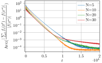
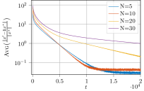
Figure 2: Cost error (left) and optimization variable error (right) in Monte Carlo simulations for varying number of agents.

Then, we perform numerical simulations over a larger network made of $N=250$ agents. We consider different optimization variable sizes, namely $n=10,20$. For each value of $N$, we generate $20$ random instances. Part of these performances have been run on the Marconi100 HPC Cluster of the Italian Cineca. We used $10$ nodes of the cluster and, for each node, we used $25$ cores and $4$ GPUs. The code has been adapted in order to perform part of the computation directly on GPUs. The results are shown in Fig. 3.In detail, increasing the number of agents increases the Lipschitz constant of the system to be averaged. Moreover, a larger domain of initial conditions also implies a potentially larger $L_{\phi}$ constant (cf. Section IV-C). This implies smaller $\gamma^{\star}$, which, fixed the other parameters, makes the convergence slower. The decision variable dimension instead impacts the selection of the dither signal. A larger number of states implies a larger number of frequencies. This, in turn, means a longer time to estimate the gradient (cf. Lemma 1). Notice that, however, the accuracy of the final estimate is guaranteed by design. Indeed, since $\delta$ and $\gamma$ are designed on $\bar{\rho}$, the trajectories of (5) converge to a ball of radius $\bar{\rho}$ independently of the problem size.

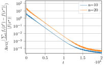
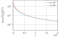
Figure 3: Cost error (left) and optimization variable error (right) in Monte Carlo simulations for different problem size and $250$ agents.

To conclude, we perform simulations with $n=30$ and $N=10$ to compare our method with the zeroth-order distributed scheme in [16]. Each agent of the algorithm in [16] estimates the local gradient with one query of the objective function at each communication round. Therefore, it is comparable to our estimation approach. The results depicted in Fig. 4 have been obtained by enforcing the same communication graphs, cost functions, and initial conditions. In detail, Fig. 4 shows that our scheme has better convergence rate and final accuracy.

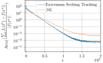
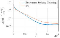
Figure 4: Cost error (left) and optimization variable error (right) comparison between the proposed algorithm and a zeroth-order scheme.

VI Conclusions

In this paper, we addressed a distributed optimization problem in which the cost function is unknown and agents have only access to local measurements. Taking inspiration from a continuous gradient tracking algorithm, we proposed a novel gradient-free distributed optimization algorithm in which gradients are estimated via extremum seeking. We analyzed the convergence properties of the proposed algorithm by using Lyapunov and averaging tools from system theory. We corroborated the theoretical analysis through Monte Carlo simulations on personalized optimization problems.

-A Proof of Lemma 1

Given $\alpha=\mathtt{col}(\alpha_{1},\dots,\alpha_{n})\in\mathbb{N}^{n}$, $y=\mathtt{col}(y_{1},\dots,y_{n})\in\mathbb{R}^{n}$, and a smooth function $f\,:\,\mathbb{R}^{n}\to\mathbb{R}$, we define

$$\alpha! :=\alpha_{1}!\dots\alpha_{n}!,\quad y^{\alpha}:=y_{1}^{\alpha_{1}}\dots y_{n}^{\alpha_{n}},$$

$$\partial^{\alpha}f(y) :=\dfrac{\partial^{\alpha_{1}}}{\partial y_{1}^{\alpha_{1}}}\dots\dfrac{\partial^{\alpha_{n}}}{\partial y_{n}^{\alpha_{n}}}f(y),\quad |\alpha|:=\alpha_{1}+\dots+\alpha_{n}.$$

Being each function $f_{i}$ smooth (cf. Assumption 3), we can apply Taylor’s expansion (cf. [41, Theorem 2]) and write

$$f_{i}(x_{i}+\delta d_{i}^{t})\! =\!f_{i}(x_{i})\!+\!\delta{d_{i}^{t}}^{\top}\nabla f_{i}(x_{i})\!+\!\frac{\delta^{2}}{2}{d_{i}^{t}}^{\top}\nabla^{2}f_{i}(x_{i})d_{i}^{t}$$

$$\hskip 11.38092pt+\delta^{3}R_{i,2}(x_{i},\delta d_{i}^{t}),$$ (38)

where the remainder $R_{i,2}(x_{i},\delta d_{i}^{t})$ is given by

$$R_{i,2}(x_{i},\delta d_{i}^{t})=\sum_{|\alpha|=3}\dfrac{\partial^{\alpha}f_{i}(x_{i}+c\delta d_{i}^{t})}{\alpha!}(\delta d_{i}^{t})^{\alpha},$$ (39)

for some $c\in(0,1)$. Then, we can use (38) to write

$$\dfrac{2}{\delta\tau_{\text{per}}}\sum_{k=t+1}^{t+\tau_{\text{per}}}d_{i}^{k}f_{i}(x_{i}+\delta d_{i}^{k})$$

$$=\dfrac{2f_{i}(x_{i})}{\delta\tau_{\text{per}}}\sum_{k=t+1}^{t+\tau_{\text{per}}}d_{i}^{k}+\left[\dfrac{2}{\tau_{\text{per}}}\sum_{k=t+1}^{t+\tau_{\text{per}}}\left(d_{i}^{k}{d_{i}^{k}}^{\top}\right)\right]\nabla f_{i}(x_{i})$$

$$\hskip 11.38092pt+\dfrac{\delta}{\tau_{\text{per}}}\sum_{k=t+1}^{t+\tau_{\text{per}}}\left(d_{i}^{k}{d_{i}^{k}}^{\top}\right)\nabla^{2}f_{i}(x_{i})d_{i}^{k}$$

$$\hskip 11.38092pt+\dfrac{2}{\delta\tau_{\text{per}}}\sum_{k=t+1}^{t+\tau_{\text{per}}}d_{i}^{k}R_{i,2}(x_{i},\delta d_{i}^{k}).$$ (40)

Since the frequencies of $d_{i}^{k}$ satisfy (4), we get

$$\sum_{k=t+1}^{t+\tau_{\text{per}}}d_{i}^{k}=0,\quad\dfrac{2}{\tau_{\text{per}}}\sum_{k=t+1}^{t+\tau_{\text{per}}}\left(d_{i}^{k}{d_{i}^{k}}^{\top}\right)=I_{n}$$

$$\sum_{k=t+1}^{t+\tau_{\text{per}}}\left(d_{i}^{k}{d_{i}^{k}}^{\top}\right)\nabla^{2}f_{i}(x_{i})d_{i}^{k}=0,$$

which combined with (40), allows us to write

$$f_{i}(x_{i}+\delta d_{i}^{t})=\nabla f_{i}(x_{i})+\dfrac{2}{\delta\tau_{\text{per}}}\sum_{k=t+1}^{t+\tau_{\text{per}}}d_{i}^{k}R_{i,2}(x_{i},\delta d_{i}^{k}).$$

The proof follows by setting $\ell_{i}(x_{i})=\dfrac{2}{\tau_{\text{per}}}\sum_{k=t+1}^{t+\tau_{\text{per}}}d_{i}^{k}R_{i,2}(x_{i},\delta d_{i}^{k})/\delta^{3}$. Finally, given a compact set $\mathcal{S}_{i}\subset{\mathbb{R}}^{n}$, let us bound $\left\|\ell_{i}(x_{i})\right\|$ for all $x_{i}\in\mathcal{S}_{i}$. Note that $\left\|\delta d_{i}^{t}\right\|\leq\delta\sqrt{n}$ for all $t\geq 0$ and let $\mathcal{S}^{\prime}_{i}\subset{\mathbb{R}}^{n}$ be a compact set such that (i) $\mathcal{S}_{i}\subseteq\mathcal{S}_{i}^{\prime}\subset{\mathbb{R}}^{n}$, and (ii) $x_{i}+\delta d_{i}^{t}\in\mathcal{S}^{\prime}$ for all $x_{i}\in\mathcal{S}_{i}$, $\delta\in(0,1]$, and $t\geq 0$. Thus, we can write

$$\sup_{\begin{subarray}{c}x_{i}\in\mathcal{S}_{i}^{\prime}\\ k\in\{1,\ldots,\tau_{\text{per}}-1\}\end{subarray}}\left\|\frac{R_{i,2}(x_{i},\delta d_{i}^{k})}{\delta^{3}}\right\|$$

$$\stackrel{{\scriptstyle(a)}}{{\leq}}\sup_{\begin{subarray}{c}x_{i}\in\mathcal{S}_{i}^{\prime}\\ k\in\{1,\ldots,\tau_{\text{per}}-1\}\end{subarray}}\left\|\frac{1}{\delta^{3}}\sum_{|\alpha|=3}\dfrac{\partial^{\alpha}f_{i}(x_{i})}{\alpha!}(\delta d_{i}^{k})^{\alpha}\right\|$$

$$\stackrel{{\scriptstyle(b)}}{{=}}\sup_{\begin{subarray}{c}x_{i}\in\mathcal{S}_{i}^{\prime}\\ k\in\{1,\ldots,\tau_{\text{per}}-1\}\end{subarray}}\left\|\sum_{|\alpha|=3}\dfrac{\partial^{\alpha}f_{i}(x_{i})}{\alpha!}(d_{i}^{k})^{\alpha}\right\|=:L_{i,\mathcal{S}_{i}}^{\prime},$$ (41)

where in $(a)$ we use the expression (39) of $R_{i,2}(x_{i},\delta d_{i}^{k})$, the definition of $\mathcal{S}_{i}^{\prime}$, and the fact that $\delta\in(0,1]$, while in $(b)$ we drop out the term $\delta^{3}$ from $(\delta d_{i}^{k})^{\alpha}$. We underline that, since the set $\mathcal{S}_{i}^{\prime}$ is compact and $f_{i}$ is smooth, $L_{i,\mathcal{S}_{i}}$ exists and is finite. The bound of $\ell_{i}(x_{i})$ follows by defining $L_{i,\mathcal{S}_{i}}:=2L_{i,\mathcal{S}_{i}}^{\prime}\sqrt{n}$ and combining the result (41) with the bound about the norm of the dither signal, i.e., $\left\|d_{i}^{t}\right\|\leq\sqrt{n}$ for all $t\geq 0$.

-B Proof of Lemma 2

In [33], it is provided a Lyapunov function proving that, under the Assumptions 1, 2, and 3, the point $\xi^{\star}=(\mathbf{1}x^{\star},\tilde{z}_{\perp}^{\text{eq}})$, with $\tilde{z}_{\perp}^{\text{eq}}:=-R^{\top}G(\mathbf{1}x^{\star})$, is a globally exponentially stable equilibrium for the continuous-time system

$$\dot{\xi}(t)=\phi_{\text{GT}}(\xi(t)).$$

In detail, in [Th. 3.1][33], it is introduced a matrix $\bar{T}\in{\mathbb{R}}^{n_{\xi}\to n_{\xi}}$ to define a change of variables $\bar{\xi}:=\bar{T}\xi$, and a matrix $\bar{P}=\bar{P}^{\top}\in{\mathbb{R}}^{n_{\xi}\times n_{\xi}}$ such that

$$\bar{a}_{1}I \leq\bar{P}\leq\bar{a}_{2}I$$ (42a)

$$(\bar{\xi}_{\text{avg}})^{\top}\bar{P}\bar{T}\phi_{\text{GT}}(\bar{T}^{-1}\bar{\xi}_{\text{avg}}) \leq-a_{3}\left\|\bar{\xi}_{\text{avg}}\right\|^{2},$$ (42b)

for all $\xi_{\text{avg}}\in{\mathbb{R}}^{(2N-1)n}$. Based on this observation, we ensure the existence of $P=P^{\top}\in{\mathbb{R}}^{n_{\xi}}$ such that

$$a_{1}I \leq P\leq a_{2}I$$ (43a)

$$\xi_{\text{avg}}^{\top}P\phi_{\text{GT}}(\xi_{\text{avg}}) \leq-a_{3}\left\|\xi_{\text{avg}}\right\|^{2},$$ (43b)

for all $\xi_{\text{avg}}\in{\mathbb{R}}^{(2N-1)n}$. With this result at hand, we define the candidate Lyapunov function $V(\xi_{\text{avg}}):=\xi_{\text{avg}}^{\top}P\xi_{\text{avg}}$ and bound $\Delta V(\xi_{\text{avg}}^{t}):=V(\xi_{\text{avg}}^{t+1})-V(\xi_{\text{avg}}^{t})$ along the trajectories of (27) as

$$\Delta V(\xi_{\text{avg}}^{t})\leq-\gamma 2a_{3}\left\|\xi_{\text{avg}}^{t}\right\|^{2}+\gamma^{2}\phi_{\text{GT}}(\xi_{\text{avg}}^{t})^{\top}P\phi_{\text{GT}}(\xi_{\text{avg}}^{t}).$$ (44)

Moreover, by using the Lipschitz continuity of the gradients of the objective functions (cf. Assumption 3) and the definition of $\phi_{\text{GT}}$, there exists $a_{4}>0$ such that

$$\left\|\phi_{\text{GT}}(\xi_{\text{avg}}^{t})\right\|\leq a_{4}\left\|\xi_{\text{avg}}^{t}\right\|.$$ (45)

Finally, for any $c\in(0,2a_{3})$, let $\gamma_{0}:=(2a_{3}-c)/(a_{2}a_{4}^{2})$ and the proof follows by using (44) and (45).

-C Proof of Lemma 3

The proof relies on (i) the matrix $P$ satisfying (28), and (ii) the fact that the norm of the perturbation term $\gamma BM_{\delta}u(\xi_{\text{avg}}^{t})$ can be arbitrarily reduced through the parameters $\delta$ as long as $\xi_{\text{avg}}^{t}$ lies into a compact set. First of all, without loss of generality, we assume $\rho\leq r_{\xi}$. Indeed, we will use the parameter $r_{\xi}$ to define a (compact) ball and arbitrarily bound the norm of the perturbation term $\gamma BM_{\delta}u(\xi_{\text{avg}}^{t})$ through the parameters $\delta$ as long as $\xi_{\text{avg}}^{t}$ lies into this ball. Hence, we can always use the more conservative condition. In detail, we define the candidate Lypaunov function $V(\xi_{\text{avg}}):=\xi_{\text{avg}}^{\top}P\xi_{\text{avg}}$ and $\Omega_{r_{\xi}}:=\{\xi_{\text{avg}}^{n_{\xi}}\mid V(\xi_{\text{avg}})\leq a_{2}r_{\xi}^{2}\}\subset{\mathbb{R}}^{n_{\xi}}$. Then, from (28a), we derive $\mathcal{B}_{r_{\xi}}\subseteq\Omega_{r_{\xi}}\subseteq\mathcal{B}_{r^{\prime}_{\xi_{\text{avg}}}}$, where $r^{\prime}_{\xi_{\text{avg}}}:=\sqrt{a_{2}/a_{1}}r_{\xi}$. Thus, it holds $\xi_{\text{avg}}^{t}\in\Omega_{r_{\xi}}$. Now, under the assumption $\xi_{\text{avg}}^{t}\in\mathcal{B}_{r_{\xi}}$ (later verified by a proper selection of the algorithm parameters), we use (44), the Cauchy-Schwarz inequality, the result (45), and the parameter $\bar{\delta}:=\max\{\delta_{1},\dots,\delta_{N}\}$, to bound $\Delta V(\xi_{\text{avg}}^{t}):=V(\xi_{\text{avg}}^{t+1})-V(\xi_{\text{avg}}^{t})$ along the trajectories of (26) as

$$\Delta V(\xi_{\text{avg}}^{t}) \leq-\gamma c_{1}\|\xi_{\text{avg}}^{t}\|^{2}+\bar{\delta}^{2}\gamma 2\left\|PB\right\|\|\xi_{\text{avg}}^{t}\|\left\|u(\xi_{\text{avg}}^{t})\right\|$$

$$\hskip 11.38092pt+\bar{\delta}^{2}\gamma^{2}2a_{4}\left\|PB\right\|\left\|\xi_{\text{avg}}^{t}\right\|\left\|u(\xi_{\text{avg}}^{t})\right\|$$

$$\hskip 11.38092pt+\bar{\delta}^{4}\gamma^{2}\left\|B^{\top}PB\right\|\left\|u(\xi_{\text{avg}}^{t})\right\|^{2}.$$ (46)

Now, let us define the compact set $\mathcal{S}_{i}:=\{x_{i}\in{\mathbb{R}}^{n}\mid\left\|x_{i}-x^{\star}\right\|\leq r^{\prime}_{\xi_{\text{avg}}}\}\subset{\mathbb{R}}^{n}$ and note that $\xi_{\text{avg}}:=(\tilde{x}_{\text{avg}},\tilde{z}_{\perp,a})\in\Omega_{r_{\xi}}\implies\tilde{x}\in\mathcal{S}\subset{\mathbb{R}}^{Nn}$, where $\mathcal{S}:=\mathcal{S}_{1}\times\dots\times\mathcal{S}_{N}$. Then, we apply result (22) to claim that, for all $i\in\{1,\ldots,N\}$, it holds $\ell_{i}(x_{i})\leq L_{i,\mathcal{S}_{i}}$ for all $x_{i}\in\mathcal{S}_{i}$. Thus, by defining $L_{\mathcal{S}}:=\max_{i}\{L_{1,\mathcal{S}_{1}},\dots,L_{N,\mathcal{S}_{N}}\}$ and using the definition $u(\xi_{\text{avg}}^{t})=\ell(\tilde{x}^{t}+\mathbf{1}x^{\star})$, we get

$$\left\|u(\xi_{\text{avg}}^{t})\right\|\leq\sqrt{N}L_{\mathcal{S}}.$$ (47)

Hence, if $\gamma\in(0,1]$ and $\delta\in(0,1]$, we can bound (46) as

$$\Delta V(\xi_{\text{avg}}^{t}) \leq-\gamma c_{1}\|\xi_{\text{avg}}^{t}\|^{2}+\gamma\bar{\delta}^{2}(b_{1}\left\|\xi_{\text{avg}}^{t}\right\|+b_{2}),$$ (48)

where we introduced

$$b_{1} :=2\left\|PB\right\|\sqrt{N}L_{\Omega_{r_{\xi}}}+2a_{4}\left\|PB\right\|\sqrt{N}L_{\Omega_{r_{\xi}}}$$

$$b_{2} :=\left\|B^{\top}PB\right\|NL_{\Omega_{r_{\xi}}}^{2}.$$

Therefore, for any $\rho\in(0,r_{\xi})$ and $c_{1}^{\prime}\in(0,c_{1})$, we define

$$\delta^{\star}_{1}:=\min\left\{\sqrt{(c_{1}-c_{1}^{\prime})\rho^{2}/(b_{1}r^{\prime}_{\xi_{\text{avg}}}+b_{2})},1\right\}.$$ (49)

Consequently, by combining (48) and (49), we claim that, if $\delta\in(0,\delta^{\star}_{1})$ for all $i\in\{1,\ldots,N\}$, then, for all $\xi_{\text{avg}}^{t}\in\Omega_{r^{\prime}_{\xi_{\text{avg}}}}$ such that $\left\|\xi_{\text{avg}}^{t}\right\|\geq\rho$, it holds

$$\Delta V(\xi_{\text{avg}}^{t})<-\gamma c_{1}^{\prime}\left\|\xi_{\text{avg}}^{t}\right\|^{2}.$$ (50)

Thus, the inequality (50) ensures that the set $\Omega_{r_{\xi}}$ is invariant for system (26). Hence, if we pick $\xi_{\text{avg}}^{0}\in\mathcal{B}_{r_{\xi}}$, we prove that $\xi_{\text{avg}}^{t}\in\Omega_{r_{\xi}}$ for all $t\geq 0$. Consequently, the bound (47) holds for all $t\geq 0$ and, in turn, also the inequality (50) is verified for all $t\geq 0$, namely we proved that the trajectories of system (26) enter the ball $\mathcal{B}_{\rho}$ exponentially fast. The result (29) follows from the inequality (50) and (28a) by setting $c_{3}:=c_{1}^{\prime}/(2a_{2})$.

References

- [1] A. Nedić and J. Liu, “Distributed optimization for control,” Ann. Rev. of Control, Robotics, and Autonomous Systems, vol. 1, pp. 77–103, 2018.
- [2] T. Yang, X. Yi, J. Wu, Y. Yuan, D. Wu, Z. Meng, Y. Hong, H. Wang, Z. Lin, and K. H. Johansson, “A survey of distributed optimization,” Annual Reviews in Control, vol. 47, pp. 278–305, 2019.
- [3] G. Notarstefano, I. Notarnicola, A. Camisa, et al., “Distributed optimization for smart cyber-physical networks,” Foundations and Trends® in Systems and Control, vol. 7, no. 3, pp. 253–383, 2019.
- [4] A. R. Conn, K. Scheinberg, and L. N. Vicente, Introduction to derivative-free optimization. SIAM, 2009.
- [5] A. Menon and J. S. Baras, “Collaborative extremum seeking for welfare optimization,” in IEEE Conf. on Decision and Contr., pp. 346–351, 2014.
- [6] M. Ye and G. Hu, “Distributed extremum seeking for constrained networked optimization and its application to energy consumption control in smart grid,” IEEE Transactions on Control Systems Technology, vol. 24, no. 6, pp. 2048–2058, 2016.
- [7] M. Guay, I. Vandermeulen, S. Dougherty, and P. J. McLellan, “Distributed extremum-seeking control over networks of dynamically coupled unstable dynamic agents,” Automatica, vol. 93, pp. 498–509, 2018.
- [8] S. Dougherty and M. Guay, “An extremum-seeking controller for distributed optimization over sensor networks,” IEEE Transactions on Automatic Control, vol. 62, no. 2, pp. 928–933, 2017.
- [9] Y. B. Salamah, L. Fiorentini, and U. Ozguner, “Cooperative extremum seeking control via sliding mode for distributed optimization,” in 2018 IEEE Conference on Decision and Control (CDC), pp. 1281–1286, 2018.
- [10] Z. Li, K. You, and S. Song, “Cooperative source seeking via networked multi-vehicle systems,” Automatica, vol. 115, p. 108853, 2020.
- [11] M. Guay, “Distributed newton seeking,” Computers & Chemical Engineering, vol. 146, p. 107206, 2021.
- [12] J. Poveda and N. Quijano, “Distributed extremum seeking for real-time resource allocation,” in American Control Conf., pp. 2772–2777, 2013.
- [13] J. Poveda, M. Benosman, and A. Teel, “Distributed extremum seeking in multi-agent systems with arbitrary switching graphs,” IFAC-PapersOnLine, vol. 50, no. 1, pp. 735–740, 2017.
- [14] S. Michalowsky, B. Gharesifard, and C. Ebenbauer, “Distributed extremum seeking over directed graphs,” in 2017 IEEE 56th Annual Conference on Decision and Control (CDC), pp. 2095–2101, 2017.
- [15] D. Wang, M. Chen, and W. Wang, “Distributed extremum seeking for optimal resource allocation and its application to economic dispatch in smart grids,” IEEE Transactions on Neural Networks and Learning Systems, vol. 30, no. 10, pp. 3161–3171, 2019.
- [16] E. Mhanna and M. Assaad, “Zero-order one-point estimate with distributed stochastic gradient-tracking technique,” arXiv preprint arXiv:2210.05618, 2022.
- [17] Y. Tang, J. Zhang, and N. Li, “Distributed zero-order algorithms for nonconvex multi-agent optimization,” IEEE Transactions on Control of Network Systems, pp. 1–1, 2020.
- [18] J. Lu and C. Y. Tang, “Zero-gradient-sum algorithms for distributed convex optimization: The continuous-time case,” IEEE Transactions on Automatic Control, vol. 57, no. 9, pp. 2348–2354, 2012.
- [19] J. Liu and W. Chen, “Sample-based zero-gradient-sum distributed consensus optimization of multi-agent systems,” in Proc. of the 11th World Congress on Intelligent Control and Automation, pp. 215–219, 2014.
- [20] D. Yuan and D. W. C. Ho, “Randomized gradient-free method for multiagent optimization over time-varying networks,” IEEE Transactions on Neural Networks and Learning Systems, vol. 26, no. 6, pp. 1342–1347, 2015.
- [21] Y. Pang and G. Hu, “Randomized gradient-free distributed optimization methods for a multiagent system with unknown cost function,” IEEE Transactions on Automatic Control, vol. 65, no. 1, pp. 333–340, 2019.
- [22] X. Chen, C. Gao, M. Zhang, and Y. Qin, “Randomized gradient-free distributed algorithms through sequential gaussian smoothing,” in 2017 36th Chinese Control Conference (CCC), pp. 8407–8412, 2017.
- [23] J. Ding, D. Yuan, G. Jiang, and Y. Zhou, “Distributed quantized gradient-free algorithm for multi-agent convex optimization,” in 29th Chinese Control And Decision Conference (CCDC), pp. 6431–6435, 2017.
- [24] Y. Pang and G. Hu, “Exact convergence of gradient-free distributed optimization method in a multi-agent system,” in 2018 IEEE Conference on Decision and Control (CDC), pp. 5728–5733, 2018.
- [25] C. Wang and X. Xie, “Design and analysis of distributed multi-agent saddle point algorithm based on gradient-free oracle,” in 2018 Australian New Zealand Control Conference (ANZCC), pp. 362–365, 2018.
- [26] L. Wang, Y. Wang, and Y. Hong, “Distributed online optimization with gradient-free design,” in Chinese Control Conf., pp. 5677–5682, 2019.
- [27] O. Bilenne, P. Mertikopoulos, and E. V. Belmega, “Fast optimization with zeroth-order feedback in distributed, multi-user mimo systems,” IEEE Transactions on Signal Processing, vol. 68, pp. 6085–6100, 2020.
- [28] Y. Pang and G. Hu, “Randomized gradient-free distributed optimization methods for a multiagent system with unknown cost function,” IEEE Transactions on Automatic Control, vol. 65, no. 1, pp. 333–340, 2020.
- [29] A. K. Sahu and S. Kar, “Decentralized zeroth-order constrained stochastic optimization algorithms: Frank–wolfe and variants with applications to black-box adversarial attacks,” Proceedings of the IEEE, vol. 108, no. 11, pp. 1890–1905, 2020.
- [30] D. Wang, J. Zhou, Z. Wang, and W. Wang, “Random gradient-free optimization for multiagent systems with communication noises under a time-varying weight balanced digraph,” IEEE Transactions on Systems, Man, and Cybernetics: Systems, vol. 50, no. 1, pp. 281–289, 2020.
- [31] I. Vandermeulen, M. Guay, and P. J. McLellan, “Discrete-time distributed extremum-seeking control over networks with unstable dynamics,” IEEE Transactions on Control of Network Systems, vol. 5, no. 3, pp. 1182–1192, 2018.
- [32] K. Kvaternik and L. Pavel, “An analytic framework for decentralized extremum seeking control,” in 2012 American Control Conference (ACC), pp. 3371–3376, IEEE, 2012.
- [33] G. Carnevale, I. Notarnicola, L. Marconi, and G. Notarstefano, “Triggered gradient tracking for asynchronous distributed optimization,” Automatica, vol. 147, p. 110726, 2023.
- [34] E.-W. Bai, L.-C. Fu, and S. S. Sastry, “Averaging analysis for discrete time and sampled data adaptive systems,” IEEE Transactions on Circuits and Systems, vol. 35, no. 2, pp. 137–148, 1988.
- [35] H. K. Khalil and J. W. Grizzle, Nonlinear systems, vol. 3. Prentice hall Upper Saddle River, NJ, 2002.
- [36] J. A. Sanders, F. Verhulst, and J. Murdock, Averaging methods in nonlinear dynamical systems, vol. 59. Springer, 2007.
- [37] J. Popenda, “On the discrete analogy of gronwall lemma,” Demonstratio Mathematica, vol. 16, no. 1, pp. 11–26, 1983.
- [38] J. M. Holte, “Discrete gronwall lemma and applications,” in MAA-NCS meeting at the University of North Dakota, vol. 24, pp. 1–7, 2009.
- [39] A. M. Ospina, A. Simonetto, and E. Dall’Anese, “Time-varying optimization of networked systems with human preferences,” IEEE Transactions on Control of Network Systems, 2022.
- [40] F. Farina, A. Camisa, A. Testa, I. Notarnicola, and G. Notarstefano, “Disropt: a python framework for distributed optimization,” IFAC-PapersOnLine, vol. 53, no. 2, pp. 2666–2671, 2020.
- [41] G. Folland, “Higher-order derivatives and taylor’s formula in several variables,” Preprint, pp. 1–4, 2005.