Photoprocessing of H₂S on dust grains: building S chains in translucent clouds and comets

Abstract

Context. Sulfur is a biogenic element used as a tracer of the evolution from interstellar clouds to stellar systems. However, most of the expected sulfur in molecular clouds remains undetected. Sulfur disappears from the gas phase in two steps. One first depletion occurs during the translucent phase, reducing the gas phase sulfur by 7-40 times, while the following freeze-out step occurs in molecular clouds, reducing it by another order of magnitude. This long-standing dilemma awaits an explanation.

Aims. The aim of this study is to understand under which form the missing sulfur is hiding in molecular clouds. The possibility that sulfur is depleted onto dust grains is considered.

Methods. Experimental simulations mimicking H₂S ice UV-photoprocessing in molecular clouds were conducted at 8 K under ultra-high vacuum. The ice was subsequently warmed up to room temperature. The ice was monitored using infrared spectroscopy and the desorbing molecules were measured by quadrupole mass spectrometry in the gas phase. Theoretical Monte Carlo simulations were performed for interpretation of the experimental results and extrapolation to the astrophysical and planetary conditions.

Results. H₂S₂ formation was observed during irradiation at 8 K. Molecules H₂S_x with $x$ ¿ 2 were also identified and found to desorb during warm-up, along with S₂ to S₄ species. Larger S_x molecules up to S₈ are refractory at room temperature and remained on the substrate forming a residue. Monte Carlo simulations were able to reproduce the molecules desorbing during warming up, and found that residues are chains or sulfur consisting of 6-7 atoms.

Conclusions. Based on the interpretation of the experimental results using our theoretical model, it is proposed that S⁺ in translucent clouds contributes notoriously to S depletion in denser regions by forming long S-chains on dust grains in few times 10⁴ years. We suggest that the S₂ to S₄ molecules observed in comets are not produced by fragmentation of these large chains. Instead, they probably come either from UV-photoprocessing of H₂S-bearing ice produced in molecular clouds or from short S chains formed during the translucent cloud phase.

1 Introduction

Sulfur is an important element for life as we know it and its chemistry is particularly relevant for linking interstellar clouds to star forming regions, to protoplanetary disks and stellar systems such as our own. S-bearing molecules are frequently used to trace the kinematics and the chemical evolution of star- (e.g. Zhou et al., 1993; Wakelam et al., 2004) and planet-forming regions (e.g. Dutrey et al., 1997; Le Gal et al., 2019). Several S-bearing species have also been recently detected in the coma of comet 67P (Calmonte et al., 2016). There is however a big problem related to sulfur chemistry, which was first recognized in the early 70s: it is not yet clear in which form most of the sulfur resides in molecular clouds. In fact, while cosmic abundances of (ionized) sulfur are found in diffuse clouds (Jenkins, 2009), the abundance of the most abundant S-bearing molecule in molecular clouds, CS, cannot be reproduced by astrochemical models, unless the S abundance in the gas phase is reduced by several orders of magnitude (e.g. Penzias et al., 1971; Oppenheimer & Dalgarno, 1974; Hasegawa et al., 1992; Bulut et al., 2021).

Several attempts have been done in the past to shed light on the ”missing sulfur” problem in molecular clouds. Caselli et al. (1994) considered the possibility that most of the S in molecular clouds is residing on the surface of dust grains; if this is the case, the rapid formation of H₂S, and the production of H₂ from the H₂S+H reaction in the ice, create a sink of H atoms, which could also explain the very slow conversion of CO ice in CH₃OH, which is indeed only observed in dense cores of molecular clouds and star-forming regions (e.g. Boogert et al., 2015; Goto et al., 2020). However, only upper limits have been measured for H₂S in ice (e.g. Smith, 1991; van der Tak et al., 2003; Jiménez-Escobar & Muñoz Caro, 2011), thus excluding that the majority of solid S is in H₂S form. Ruffle et al. (1999) proposed that most of the S depletion happens in translucent clouds, where S atoms are still mainly in atomic ionized form (see also Sternberg & Dalgarno, 1995) while the dust grains are mainly negatively charged; in this scenario, the Coulomb-enhanced freeze-out rate of S⁺ will rapidly deplete sulfur from the gas phase (see also Umebayashi & Nakano, 1980, for generic cations). Vidal et al. (2017) compared their astrochemical modeling results to observations toward the TMC-1(CP) dark cloud and concluded that, depending on the cloud age, most of the sulfur could be either in (the not observable) atomic form or on HS and H₂S in solid form. Laas & Caselli (2019) expanded the chemistry of sulfur by including S-bearing organic molecules and the Ruffle et al. (1999) freeze-out mechanism; they found a good agreement with observations in molecular clouds and concluded that the majority of S is trapped in organo-sulfur species in icy mantles of dust grains.

In laboratory experiments where H₂S ice is irradiated either with UV photons or energetic particles (proxy for the interstellar cosmic rays), it has been found that a significant fraction of H₂S can be transformed in allotropic forms of S, including the most stable form S₈ (e.g. Jiménez-Escobar & Muñoz Caro, 2011; Jiménez-Escobar et al., 2014). This has also been confirmed theoretically by Shingledecker et al. (2020) using astrochemical models inclusive of radiation chemistry; interestingly, these models predict that the impact of energetic particles in H₂S-rich ices reduces the abundance of H₂S, while enhancing SO₂, OCS and S₈. The first interstellar molecule containing more than one S atom (S₂H) was detected recently by Fuente et al. (2017) toward the Horsehead photodissociation region, suggesting an interesting interplay between gas-phase and surface chemistry. The GEMS large project (Rodríguez-Baras et al., 2021) at the IRAM 30m telescope is also providing important observational constraints on sulfur chemistry in molecular clouds; for example Navarro-Almaida et al. (2020) measured gas-phase H₂S across several sources, finding good agreement with chemical models assuming non depleted S abundances, which however highly overestimate the CS abundance. With the ROSINA instrument onboard Rosetta, Calmonte et al. (2016) measured a variety of S-bearing molecules in comet 67P, which appears to preserve pre-stellar ice (Altwegg et al., 2019; Drozdovskaya et al., 2019, 2021): the majority of S is in H₂S ice (about 57%), followed by atomic S, SO₂, SO, OCS, H₂CS, CH₃SH, CS₂, S₂ and other S-bearing organics.

Despite the many observations and chemical models available, there are still many open questions about sulfur chemistry in the interstellar medium: what happens to S atoms when adsorbed onto dust grains in translucent and molecular clouds? What is the chemistry of irradiated H₂S ice? Which fraction of sulfur atoms will form chains? Which S-bearing molecules should be observed to test the models? In this paper we focus our attention on detailed experimental work and its simulation with a Monte Carlo chemical model, with the aim of putting quantitative constraints on the S depletion and chemical processing in translucent and molecular clouds.

The paper is structured as follows: Section 2 describes the laboratory experiments and Section 3 presents the results of the experimental work; Monte Carlo simulations are described in Section 4. Section 5 discusses photo-processes of H₂S ice in simulations and experimental work, while applications to interstellar molecular clouds and to Solar System conditions can be found in Sections 6 and 7, respectively. Our conclusions are in Section 8.

2 Experiments: H₂S irradiation with UV photons

The experimental results presented here have been obtained using the InterStellar Astrochemistry Chamber (ISAC) at the Centro de Astrobiología (Muñoz Caro et al., 2010). ISAC is an ultra-high vacuum (UHV) chamber with a base pressure dominated by background H₂ in the range $P$ = 2.5-4.0 x 10^-11 mbar, which corresponds to dense cloud interiors. H₂S ice samples were grown by accretion of gas molecules onto the tip of a cold finger at 8 K, where a MgF₂ infrared (IR) and ultraviolet (UV) transparent window serves as the substrate for deposition. This temperature was achieved by means of a closed-cycle helium cryostat. The samples were then warmed up until a complete sublimation was attained. A silicon diode temperature sensor, and a LakeShore Model 331 temperature controller are used, reaching an accuracy of about 0.1 K.

The evolution of the solid sample was monitored by in situ transmittance Fourier Transform Infrared spectroscopy (FTIR) with a spectral resolution of 2 cm^-1. Column densities of each species in the ice were calculated from the IR spectra using the formula

$$N=\frac{1}{A}\int_{band}{\tau_{\nu}d\nu},$$ (1)

where $N$ is the column density in cm^-2, ${\tau}_{\nu}$ the optical depth of the band, $d\nu$ the wavenumber differential in cm^-1, and $A$ the band strength in cm molecule^-1. The integrated absorbance is equal to 0.43 $\times$ $\tau$, where $\tau$ is the integrated optical depth of the band. The adopted band strengths, $A$, derived from laboratory experiments are provided in Table 1.

Species	Feature	Position	Position	$A$$\times$ 10-17
		$\mu$m	cm-1	cm molec-1
H2S	S-H stretch	3.940	2538	2.0 a
H2S2	S-H stretch	4.016	2490	2.4$\pm$0.5 b

^a Jiménez-Escobar & Muñoz Caro (2011)
^b This work. Band strength of H₂S₂ was calculated between 100 K and 120 K, showing a constant value in this range, see Sect. 3.2.

Table 1: Photo-dissociation reactions with associated rates considered in the present study. These rates are taken from Shingledecker et al. (2020).

The accretion rate measured by IR spectroscopy of the deposited ice was 1 ML s^-1. Samples were UV-irradiated using a microwave-stimulated hydrogen flow discharge lamp (MDHL) that provides a flux of 2.5 $\times$ 10¹⁴ photons cm^-2 s^-1 at the sample position with an average photon energy of 8.6 eV. The MDHL spectrum is reported in Cruz-Diaz et al. (2014). UV spectra were measured routinely in situ during the experiments with the use of a McPherson 0.2 meter focal length VUV monochromator (Model 234/302) with a photomultiplier tube (PMT) detector equipped with a sodium salicylate window, optimized to operate from 100-500 nm (11.27-2.47 eV), with a spectral resolution of 0.4 nm. UV absorption spectra of H₂S ice samples served to monitor the detection of photoproducts generated upon UV-irradiation at 8 K or later during warm-up. For more details on the experimental protocol employed for VUV spectroscopy, see Cruz-Diaz et al. (2014).

3 Experimental results

As reported by Jiménez-Escobar & Muñoz Caro (2011), thermal processing of H₂S ice leads to crystallization at temperatures above 40 K. This process reduces the number of randomly oriented molecules and the vibration modes become narrower, see inlet of Fig. 1, which agrees with Fig. 1 in Jiménez-Escobar & Muñoz Caro (2011). The antisymmetric and symmetric vibrations appear at 2553 and 2530 cm^-1, respectively. The remaining amorphous domains are responsible for the IR band centered at 2538 cm^-1.

3.1 Photoproduct formation in UV-irradiated H₂S ice

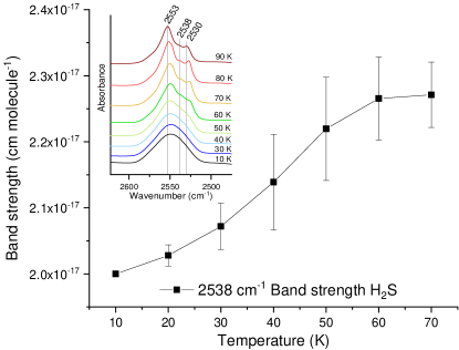
Figure 1: Evolution of the H₂S band strength as a function of temperature. Above 70 K, thermal desorption becomes important, reducing H₂S column density, preventing us from a quantification of the band strength.

UV-irradiation of H₂S ice samples produces HS$\cdot$ radicals very readily, according to Reaction 2. HS$\cdot$ radicals can also react with hydrogen atoms in the backwards reaction to reform the original H₂S molecule. IR spectroscopy shows that H₂S is dissociated along the first steps of UV irradiation, when recombination to form H₂S is inhibited, as a consequence of the low abundance of HS$\cdot$ radicals. For larger irradiation periods, however, H₂S recombination takes place, reducing the overall H₂S dissociation.

$$\rm{H}_{2}\rm{S}\thinspace\rightleftharpoons\thinspace\rm{HS\cdot}\thinspace+\thinspace\rm{H\cdot}$$ (2)

The rapid formation of HS$\cdot$ radicals favors Reaction 3 to produce H₂S₂ molecules as well as a second hydrogen elimination (Reaction 4) forming S atoms. H₂S₂ molecules were detected at 8 K by IR spectroscopy through its H-S stretching mode centered at 2485 cm^-1 (Isoniemi et al., 1999). On the other hand, S atoms can only be detected during the warm-up phase (see Sect. 3.2).

$$2\thinspace\rm{HS\cdot}\thinspace\xrightarrow{}\thinspace\rm{H_{2}S_{2}}$$ (3)

$$\rm{HS\cdot}\thinspace\xrightarrow{}\thinspace\rm{S}\thinspace+\thinspace\rm{H\cdot}$$ (4)

The rapid formation of H₂S₂ enables further reactions. H₂S₂ molecules can be dissociated by UV-photons according to Reaction 5. H₂S₂ molecules can also recombine with HS$\cdot$ radicals to produce H₂S₃ molecules (Reaction 6).

$$\rm{H_{2}S_{2}}\thinspace\xrightarrow{}\thinspace\rm{H_{2}S\cdot}\thinspace+\thinspace\rm{H\cdot}$$ (5)

$$\rm{H_{2}S_{2}}\thinspace+\thinspace\rm{HS\cdot}\thinspace\xrightarrow{}\thinspace\rm{H_{2}S_{3}}$$ (6)

Finally, H₂S₄ was also detected in our experiments. The presence of HS${}_{3}\cdot$ radicals will produce H₂S₄ by reaction with the abundant HS$\cdot$ radical (Reaction 7). Secondly, 2 HS${}_{2}\cdot$ radicals can react producing H₂S₄ molecules (Reaction 8). The relatively low abundance of HS${}_{3}\cdot$ radicals, and the low probability of 2 HS${}_{2}\cdot$ radical-radical reactions in an environment dominated by HS$\cdot$ radicals determine the low formation rate of H₂S₄ molecules. Nevertheless, H₂S₄ was detected during warm-up of the irradiated H₂S ice by quadrupole mass spectrometry (QMS), as explained in Sect. 3.2.

$$\rm{HS\cdot}\thinspace+\thinspace\rm{HS_{3}\cdot}\thinspace\xrightarrow{}\thinspace\rm{H_{2}S_{4}}$$ (7)

$$2\thinspace\rm{HS_{2}\cdot}\thinspace\xrightarrow{}\thinspace\rm{H_{2}S_{4}}\thinspace$$ (8)

Non-hydrogenated molecules can also be formed. Reaction between S atoms produces S₂ molecules. Further S atom additions, as well as dehydrogenation of H₂S_x species can lead to larger S_x molecules. Some S_x species do not absorb in the IR and others display only very weak absorption bands. These products could not be detected by IR spectroscopy in our experiments, but they were measured by QMS during warm-up.

3.2 Warm-up of UV-irradiated H₂S ice

Some of the radical species made during UV irradiation of H₂S ice react at low temperatures, such as HS$\cdot$ radicals, while larger radical species may remain in the ice matrix until thermal energy during warm-up enables subsequent reactions. IR spectroscopy confirmed the production of H₂S₂ molecules at 8 K (Isoniemi et al., 1999). Overlapping of H-S IR stretching modes of H₂S₂ with those of larger H₂S_x species, expected to present lower formation rates, hindered the estimation of their formation temperatures.

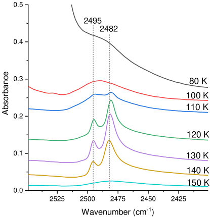
Figure 2: IR spectra collected during warm-up of a previously UV-irradiated H₂S ice sample. After sublimation near 90 K of most H₂S molecules, H₂S₂ molecules are allowed to interact forming a crystalline structure. Crystallization leads to narrowing of the antisymmetric and symmetric vibrations of H₂S₂ that appear at 2495 and 2482 cm^-1, respectively.

After the sublimation of amorphous and crystalline H₂S molecules at 96 K, IR spectra show the crystallization of H₂S₂ (Fig. 2). From the IR band centered around 2490 cm^-1, two absorption features can be clearly distinguished at temperatures between 110 K and 150 K. These bands belong to the antisymmetric (2495 cm^-1) and the symmetric (2482 cm^-1) vibration modes of H₂S₂. Zengin & Giguère (1959) measured the IR spectrum of crystalline H₂S₂, reporting values in close agreement with our experiments and the work reported by Moore et al. (2007).

The band strength of the H₂S₂ IR band at 2490 cm^-1 was estimated as follows. Martín-Doménech et al. (2015) provided a method to calculate the column density of a given species from the integrated QMS signal, after calibrating the QMS by using CO ice, by applying Eq. 9, where $N(mol)$ is the column density of a given species in molec $\cdot$ cm^-2, $A\left(\frac{m}{z}\right)$ is the integrated area taken from the QMS, $k_{CO}$ is the proportionality constant from the calibration of the QMS in a CO ice irradiation experiment leading to photodesorption of the CO molecules, $\sigma^{+}$(mol) is the ionization cross-section of each species ionized at a voltage of 70 eV in the QMS (data adopted from the National Institute of Standards and Technology), $IF(z)$ is the ionization factor, which has been considered unity for all molecules, $FF$ is the fragmentation factor, derived from the QMS spectrum of each species, and $S\left(\frac{m}{z}\right)$ is the sensitivity of the QMS (Martín-Doménech et al., 2015).

$$N(mol)=\frac{A\left(\frac{m}{z}\right)}{k_{CO}}\cdot\frac{\sigma^{+}(CO)}{\sigma^{+}(mol)}\cdot\frac{IF(CO^{+})}{IF(z)}\cdot\frac{FF(28)}{FF(m)}\cdot\frac{S(28)}{S(\frac{m}{z})}\\$$ (9)

Then, the ratio between column density of H₂S and H₂S₂ (R${}_{\frac{H_{2}S}{H_{2}S_{2}}}$) can be obtained from the QMS during thermal desorption of H₂S and H₂S₂, using Eq. 10, and taking the area below the thermal desorption peak in the QMS:

$$R_{\frac{H_{2}S}{H_{2}S_{2}}}=\frac{N(H_{2}S)}{N(H_{2}S_{2})}=\frac{A(34)}{A(66)}\cdot\frac{\sigma^{+}(H_{2}S_{2})}{\sigma^{+}(H_{2}S)}\cdot\frac{IF(H_{2}S_{2}^{+})}{IF(H_{2}S^{+})}\cdot\frac{FF(66)}{FF(34)}\cdot\frac{S(66)}{S(34)}\\$$ (10)

The band strength of the 2490 cm^-1 IR feature of H₂S₂ can be finally obtained assuming that $\sigma^{+}(H_{2}S_{2})$ = $\sigma^{+}(H_{2}S)$, as there is no reported value for $\sigma^{+}(H_{2}S_{2})$, and calculating the column density of H₂S from IR data before its thermal desorption:

$$N(H_{2}S_{2})=\frac{1}{R_{\frac{H_{2}S}{H_{2}S_{2}}}}\cdot N(H_{2}S)$$ (11)

Because the factor $k_{CO}$ cancels out and does not appear in Eq. 10, this method reduces the error due to i) variation in the QMS sensitivity between the CO photodesorption experiment and the H₂S irradiation experiment due to degradation of the QMS filament with time and ii) different environmental conditions between those experiments, since the measurement of the reference species, H₂S, and that of the target molecule, H₂S₂, were made during the same experiment. Entering the estimated values of $N$(H₂S₂) and its corresponding integrated IR absorption in Eq. 1, an IR band strength value of $A$(H₂S₂) = 2.4$\pm$0.5 $\times$ 10^-17 cm molecule^-1 was obtained.

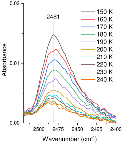
Figure 3: IR spectra acquired during warm-up of previously irradiated H₂S ice. This band is evidence for the presence of H₂S_x molecules with $x$ ¿ 2 that were detected during desorption in the gas phase by QMS, H₂S₃ and H₂S₄ desorbing at temperatures below 225 K, see Fig. 4. Therefore, the small IR absorption that remains above 240 K is likely due to H₂S_x species with $x$ ¿ 4 that are refractory at this temperature and could thus not be detected by the QMS.

After thermal desorption of H₂S₂, a new IR feature becomes visible at 2481 cm^-1 (Fig. 3). This IR band disappears gradually above 150 K during the TPD, suggesting that H-S stretching modes from species less volatile than H₂S₂ contribute to this vibration mode.

Fig. 4 shows the thermal desorption of H₂S_x molecules. Two peaks are clearly observed during H₂S thermal desorption. A first desorption peak appearing at 88 K coincides with the disappearance of the 2538 cm^-1 IR feature between 80 K and 90 K in Fig. 1, that is, thermal desorption of amorphous H₂S molecules. More stable crystalline H₂S molecules sublimate at slightly larger temperatures, producing a second peak at 96 K, see Fig. 4.

Furthermore, QMS data in Fig. 4 shows evidence for H₂S₂ desorption, $\frac{m}{z}=66$, with a maximum at 144 K, which coincides with the disappearance of the IR features at 2495 and 2482 cm^-1 attributed to this species.

The better sensitivity of QMS compared to IR spectroscopy allowed the identification of larger species during ice warm-up. Fig. 4 shows a maximum of $\frac{m}{z}=98$ at 184 K related to desorbing H₂S₃ molecules, and the peak of $\frac{m}{z}=130$ at 204 K corresponds to thermally desorbed H₂S₄. The latter identification of H₂S₄ was confirmed in several irradiation and warm-up experiments.

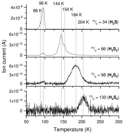
Figure 4: Thermal programmed desorption (TPD) of an irradiated H₂S ice sample. Up to 4 different H₂S_x species were detected with decreasing abundances. Most intense $\frac{m}{z}$ fragment for all the species is shown.

The fragmentation of desorbing H₂S_x species when they impact the filament of the QMS can lead to S${}_{x}^{+}$ fragments that might be erroneously attributed to the desorption of S_x species formed in the ice. Nevertheless, this was not a problem since the m/z values of S_x molecules were detected at temperatures that did not overlap significantly with those of H₂S_x species. Fig. 5 shows the thermal desorption of S_x species. Thermal desorption of S atoms reaches its maximum at 58 K, dragging some S₂ molecules during this process. The main desorption of S₂ molecules takes place at 113 K. If we assume that the molecular mass is the main factor determining the desorption temperature, S₃ molecules are expected to desorb around 180-200 K, but they were not detected in our experiments. The non-detection of S₃ and the detection of S₄, with a maximum of desorption at 283 K, suggests that a preferential formation scheme encompass the dimerization of S₂ molecules, favoring the formation of S_x species with a pair number of S atoms.

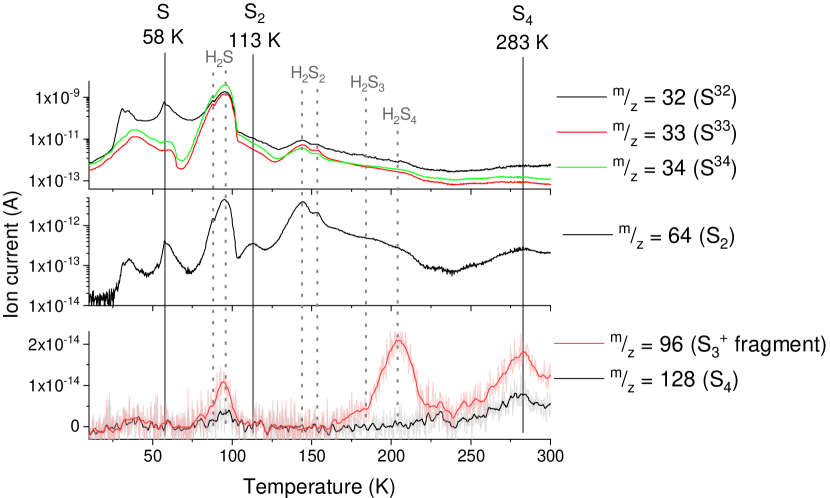
Figure 5: TPD of an irradiated H₂S ice sample. It should be noted that a given m/z value can correspond to the molecular ion of a species or to a fragment of a larger species. The desorption temperatures of S_x molecules correspond to the solid vertical lines. Dashed lines indicate the desorption of H₂S_x species. Apart from the molecular ion of each species, $\frac{m}{z}$ values of the main fragments used to confirm the presence of these species are displayed.

4 Monte Carlo simulations

We used a step-by-step Monte Carlo simulation to follow the deposition of H₂S molecules on the surface as well as their photo-dissociation into other products. Our model is described in Cazaux et al. (2015, 2017). H₂S molecules originating from the gas phase arrive at a random time and location on the substrate, which is represented as a grid, and follow a random walk. The arrival time depends on the rate at which gas species collide with the surface. The molecules arriving on the surface can be bound to the substrate and to other H₂S, HS or S species via van der Waals interactions. In the present study we use on-lattice KMC simulations. Other types of simulations, such as off-lattice KMC method allow to determine the distance of the species explicitly (Garrod, 2013). In the present study, we consider the distance between two adsorption sites (and therefore the distance between two adjacent adsorbed species) to be equal for the entire grid, and concentrate on defining the reactions occurring within the chemical species that are deposited on the surface (H₂S) or are produced by photo-dissociation reactions. Our model is meant to constrain the experimental results as accurately as possible, before being exported to interstellar medium conditions in sections 6 and 7.
The different mechanisms used in this model are accretion, diffusion, sublimation, chemical reactions and photo-dissociation. These different mechanisms (accretion, diffusion and sublimation) occur at rates which have been described in a previous work (Cazaux et al., 2018). The accretion rate in number of molecules per second is

$$R_{\rm{H_{2}S}}=n_{\rm{H_{2}S}}\rm{V}_{\rm{H_{2}S}}\ \sigma\ \rm{Stick},$$ (12)

where V${}_{\rm{H_{2}S}}=\sqrt{\frac{8\ k\ T_{\rm{gas}}}{\pi\ m_{\rm{H_{2}S}}}}\sim 2.5\times 10^{4}\sqrt{\frac{T_{\rm{gas}}}{100}}$ cm s^-1 is the thermal velocity of H₂S, and $\sigma$, the cross-section of the surface. Stick is the sticking coefficient that we consider to be unity in this study. The distance between two sites is assumed to be 3 Å, which is consistent with the density of the number of sites typically assumed on surfaces N_S = $({3\AA})^{-2}$ $\sim$ 10¹⁵ cm^-2. The cross-section scales with the size of the grid considered in our calculations (which is 40$\times$40 sites) as $\sigma\sim(3\ 10^{-8}\times 40)^{2}$ cm²= 1.4  10^-12 cm². The accretion rate of H₂S molecules in the experiment is 1ML/s. In our calculations, the accretion rate in ML/s can be written as R${}_{\rm{H_{2}S}}=\frac{n_{\rm{H_{2}S}}\rm{V}_{\rm{H_{2}S}}}{NS}$ ML/s. Therefore, we chose the density of H₂S in our simulations to be around $n_{\rm{H_{2}S}}\sim 10^{10}$ cm^-3 in order to reproduce experimental conditions.

The diffusion from one site to another one is described in previous work (Cazaux et al., 2017). In the present study, we consider an alpha coefficient, e.g. the ratio between diffusion barriers and thermal desorption barriers, of 0.9. Such slow diffusion was determined in previous work (Cazaux et al., 2017) and is considered in the present study.

In the present work, we also consider photo-dissociation reactions as well as the reactions between the photo-products. These mechanisms are described in the following subsections.

4.1 Photo-dissociation reactions

Once a photon is absorbed by a H₂S molecule, it will dissociate it in HS + H. The product of the reaction, HS, can also receive a photon and be dissociated further in S + H. For our model, the dissociation rates are taken from Shingledecker et al. (2020) and are reported in Table 2. As the photo-dissociation of H₂S can produce S atoms, these S atoms can find each other and make chains, which increases their binding energies and lowers their photo-dissociation rates as shown in Table 2. The rates are computed as follow:

$$R_{diss}=G_{0}*A\exp(-B\times Av).$$ (13)

In the experiments, each H₂S molecule receives a photon every 10 seconds. The parameter G₀ is the Habing radiation field (Habing, 1968) which is the far ultraviolet (FUV) radiation field (where 1 G₀ equals a flux of 1.6 $\times$ 10^-3 erg cm^-2 s^-1, which is equivalent to 2$\times$ 10⁷ cm^-2 s^-1). In order to have 0.1 photon per second, to mimic experimental conditions, we use G₀=5$\times$ 10⁶. The dissociation rate of H₂S molecules is therefore R_diss= 0.015 s^-1 for H₂S and is of 0.006 s^-1 for HS.

React1	React2	Prod1	Prod2	A	B
HS	Photon	H	S	0.12E-08	2.4
H2S	Photon	H	HS	0.31E-08	2.6
H2S2	Photon	H	HS	0.55E-09	1.7
H2S2	Photon	H	HS	0.45E-09	1.7
S2	Photon	S	S	0.6E-09	1.9
S3	Photon	S2	S	0.1E-09	0.0
S4	Photon	S3	S	0.8E-10	0.0
S5	Photon	S4	S	0.5E-10	0.0
S6	Photon	S5	S	0.1E-10	0.0

Table 2: Photo-dissociation reactions with associated rates considered in the present study. These rates are taken from Shingledecker et al. (2020).

4.2 Chemical reactions

In the present simulations, we consider that species present in the solid phase (on the surface or in the ice) can react with each other. We consider a small solid phase chemical network allowing 5 possible reactions, and report the associated pre-exponential factors and barriers in table 3. These reactions have been selected in the chemical network from Shingledecker et al. (2019). In the present study we do not consider chemical desorption.

React1	React2	Prod1	Prod2	$\nu$ (s-1)	Ea(K)
H	H	H2		1E12	0
H	S	HS		1E12	0
H	HS	H2S		1E12	0
H	H2S	H2	HS	1E12	1530
H	HS	H2	S	1E12	0

Table 3: Reactions considered in the present study. Reactions are taken from Shingledecker et al. (2020).

4.3 Binding energies

The binding energies of S atoms, as well as H, H₂, HS, H₂S and S-chains are reported in Table 4. The binding energies for the S-chains are extrapolated by using the S-chains observed in the experiments. S₄ desorbs at 283 K (which implies a binding energy of $\sim$8490 K) while S₃ desorbs around 200 K (binding energy of $\sim$6000 K). These binding energies are reported in Table 4. This means that the difference in desorption peak in the TPD when a S is added is around 80 K, which corresponds to a additional binding energy due to an additional S atom to the chain around  2400 K. We take this value as an addition to the binding energy of the S-chain when an extra S atom is added. We therefore reach a binding energy of 18000 K for S₈. It should be noted that this is a simple assumption, and the change in binding energy could become less with the number of S atoms added, as this is the case in clusters (Lin et al., 2005).

Species	Binding	Reference
	energy
	(K)
H	500	Dulieu et al. 2005
H2	400	Dulieu et al. 2005
H2S	2640	Jiménez-Escobar & Muñoz Caro 2011
HS	1100	Wakelam et al. 2017
S	1800	Wakelam et al. 2017
HS2	4264	Jiménez-Escobar & Muñoz Caro 2011
	5500	Jiménez-Escobar & Muñoz Caro 2011
S2	3390	this work
S3	6000	this work
S4	8490	this work
S5	10800	extrapolation
S6	13200
S7	15600
S8	18000

Table 4: Species considered in this study with their associated binding energies. Note that 2 values of HS₂ correspond to the 2 desorption peaks in the TPD implying different orientation of the molecules.

4.4 Results

4.4.1 TPD simulations of H₂S

We performed Monte Carlo simulations for the deposition and irradiation of H₂S in order to reproduce the experimental measurements. We first performed simulations without irradiation in order to reproduce a simple experimental TPD curve. Our results are reported in Figure 6. In this figure, we are able to reproduce the two peaks located around 88 K and 96 K as found in Fig. 4. To reproduce these two peaks, we considered binding energies of species in Table 4. In our calculations, the strongest interaction between a species with a neighbor is considered. However, the width of the peaks seen in the experiments are of few tens of K. This implies that the binding energy is not a single value but a distribution of values. To reproduce the width of the peak, we consider the strongest interaction of the species (from Table 4) and add the contribution of the neighbors around the considered species for 2% (this value is taken as it reproduces the width the best). For example, an H₂S molecule bound with 2 neighbors would have a binding energy of 2640 + 0.02 $\times$ 2640 = 2693 K. This allows to take into account the fact that the binding energy is increased if more neighbors are involved.

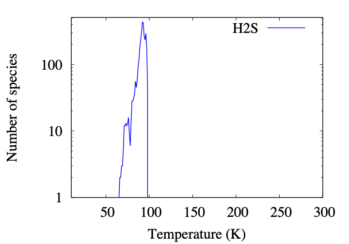
Figure 6: TPD of H₂S with MC simulations.

4.4.2 TPD simulations of irradiated H₂S: case without ice self shielding

In these simulations, we deposit H₂S on the surface and irradiate the molecules with UV photons in rates similar to experimental rates. The vizualisation of our Monte Carlo simulations for different surface temperature is presented in Figure 7. In this figure, we show the grid of 40 by 40 sites. Each cube shows one species, the color allowing to identify the species. The H₂S molecules are presented in yellow, the HS in green and S atoms in blue. The first panel represents the H₂S after deposition, while the second, third, fourth and fifth panels show the coverage of the surface during the TPD at 50, 100, 200 and 300 K respectively. Our results show that after deposition, the H₂S layers have not interacted much with the photons since most of the ice is yellow (and traces of green and blue). The deposition in our simulation takes around 8 seconds, and the molecules receive a photon every 10 seconds. This means that the number of products due to photo-dissociation are less important during the deposition that during the TPD (in our simulations). This is reflected by the composition of the surface at 8 K, showing that most of H₂S molecules are still present on the surface with a minority of HS and S species. The surface at 50 K, shown in the top middle panel of Figure 7, illustrates a longer irradiation time, since the time spent after deposition is 42 minutes. The photo-dissociation rate of H₂S is R_diss = 0.015 s^-1 in our simulations, which implies that one H₂S molecule would not survive such a long time since in 42 minutes it would have received around 40 photons, and the first photon would have already dissociated the molecule in HS + S. The surface coverage at 50 K is therefore mainly composed of S atoms but also HS and few H₂S. The photo-products HS and S are dominating compared to the coverage at 8 K after deposition. In Figure 7, top right panel, the surface temperature is of 100 K. Most of the H₂S and HS have desorbed from the surface, and mostly S atoms are present. The species are organized as chains, which allow them to have larger binding energies compared to individual species. These binding energies are reported in Table 4. For high temperatures, only chains can still be present on the surface. The bottom left panel of Figure 7 shows the surface at 150 K. Only chains with S atoms and sometimes an inclusion of HS or H₂S can be observed. At 300 K, on the bottom middle panel, only few chains are remaining on the surface and all other species have desorbed. These residues in our simulations under the form of chains cannot be seen experimentally in the TPD because their binding energies are too high. In our simulations, the longest chain has 7 S atoms, and few chains have 6 S atoms. The bottom right panel shows the same simulation and temperature than the bottom middle panel, but in this case the chains are highlighted by different colors while in the previous figures, the colors were showing which species were composing the chain (S, HS or H₂S). We can clearly see that some chains can reach a maximum of around 6-7 S atoms in the present conditions.

In order to compare our results to the experimental measurements from Fig. 2, we present in Figure 8 the simulated number of desorbed species during the TPD. Our results show different peaks that are attributed to S atoms, S chains as well as HS, H₂S and H₂S₂. This TPD agrees very well with the experimental results, showing chains with up to 4 members. In the present simulations, we used a coverage of few 3–5 ML (see top left panel of Figure 7). This differs from the experimental conditions where thousands of monolayers were deposited on the surface. The ratios between the different peaks of the TPD would change significantly if the simulations were run for high H₂S ice thickness. Our model however, cannot compute such thick ices, but in the present study we can compare the temperature of the desorption peaks in the TPD and estimate the residuals remaining in the surface at high temperatures.

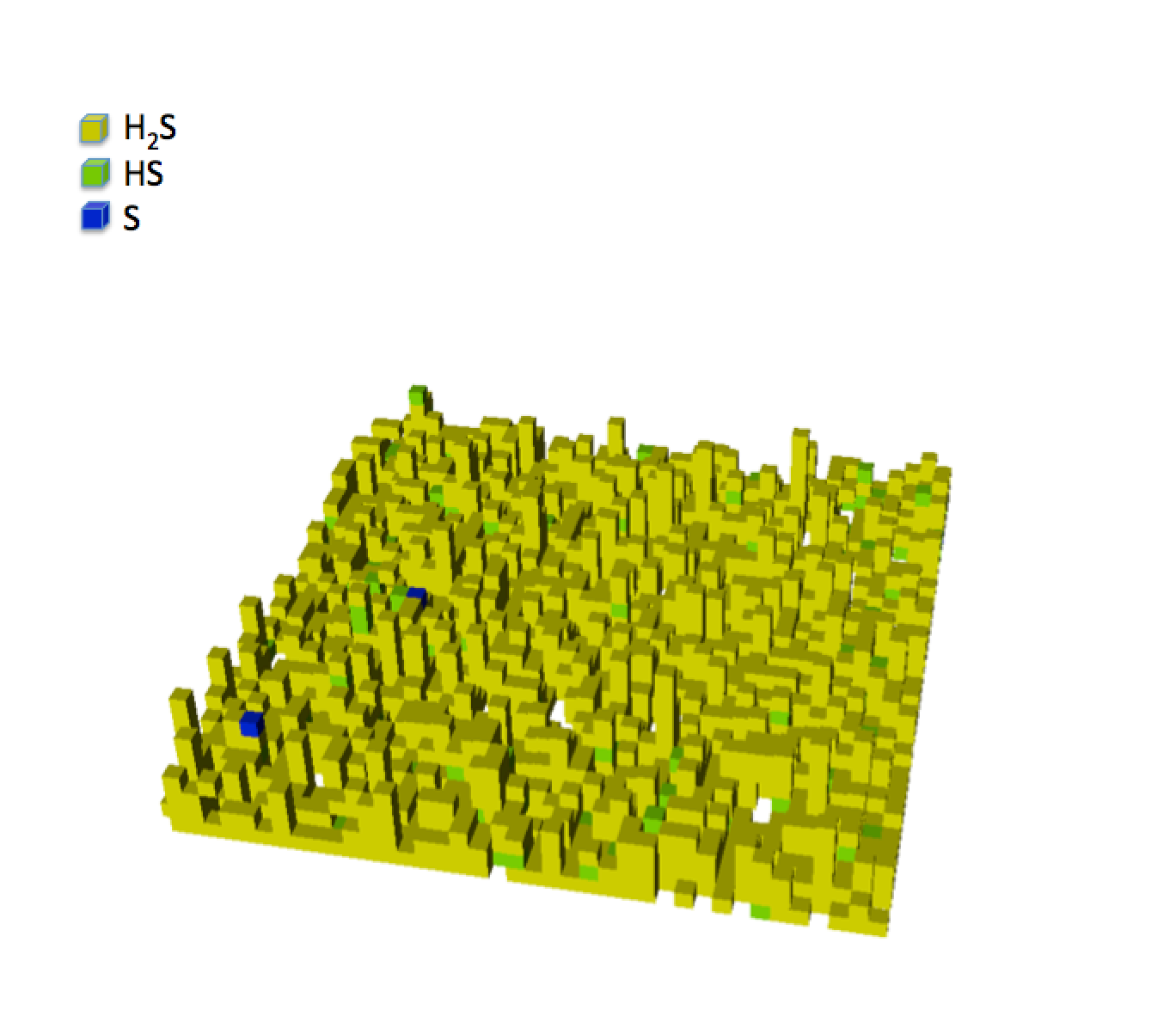
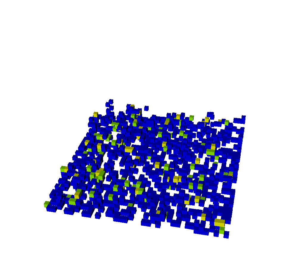
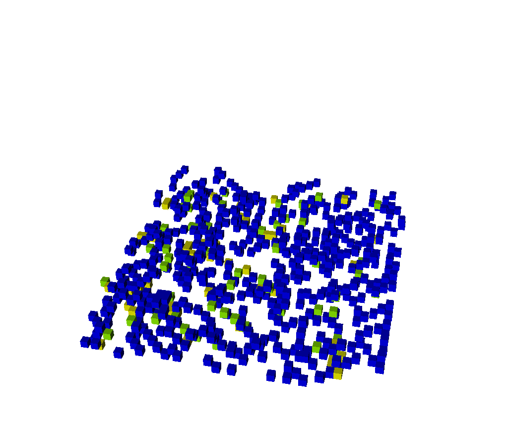
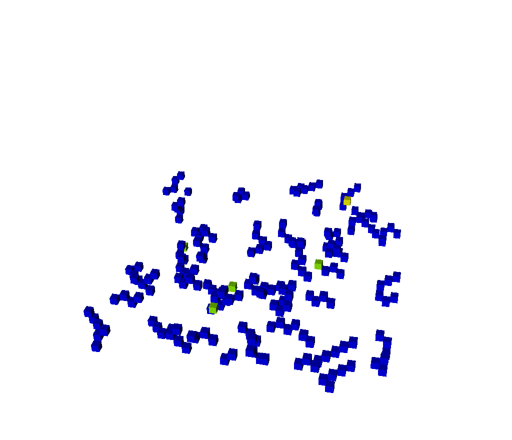
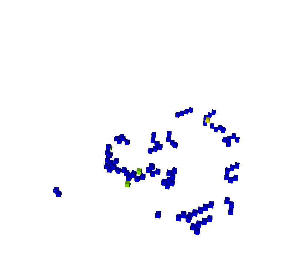
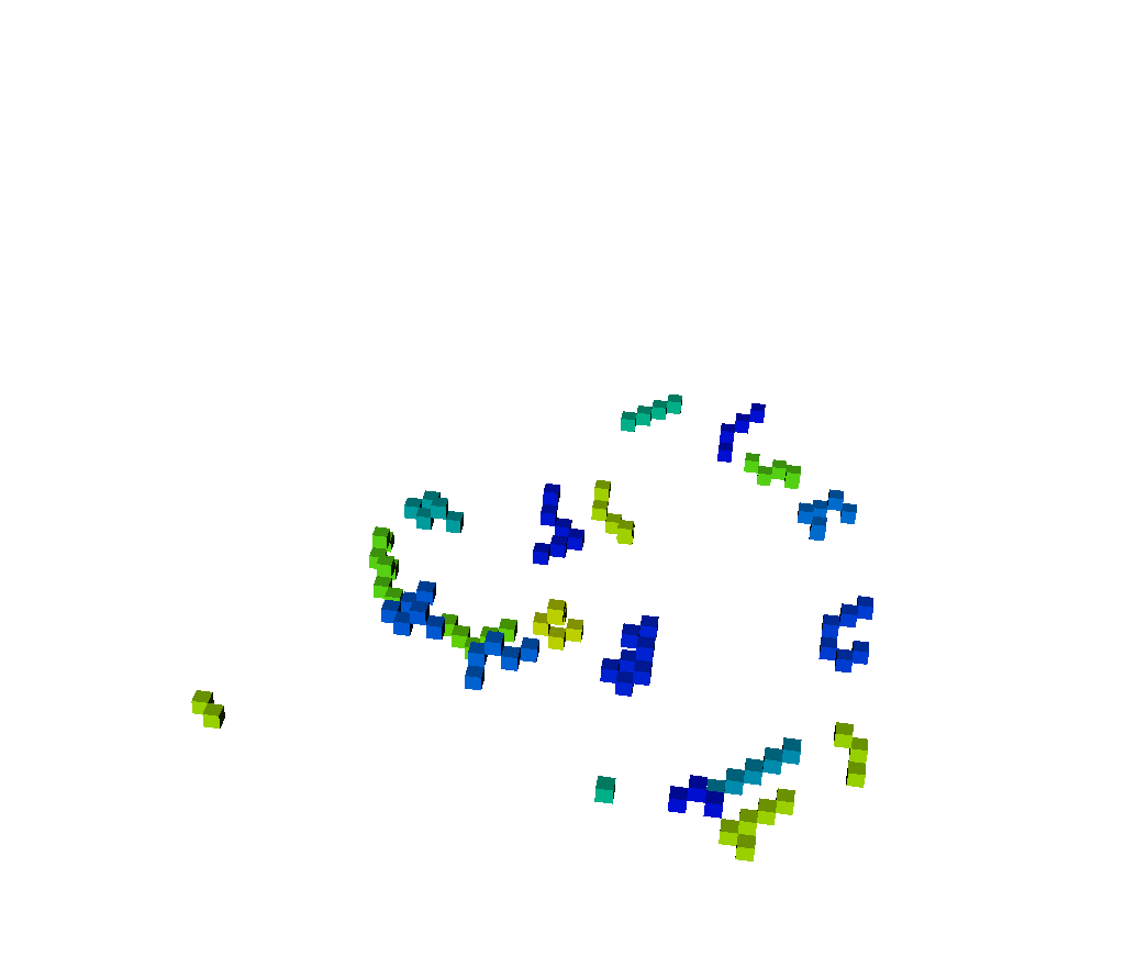
Figure 7: H₂S on the surface after deposition at 8 K (top left) and during TPD at 50 K (top middle), at 100 K, (top right), at 200 K (bottom left) and 300 K (bottom middle). The bottom right panel also shows the surface at 300 K but with the chains being highlighted by using one color per chain. In these simulations, the molecules in the ice do not shield each other and photons can therefore dissociate molecules from the top layers to the bottom layers. The deposition rate of H₂S is 1ML/s, the heating ramp is 1K/min and G₀=5 $\times$ 10⁶.

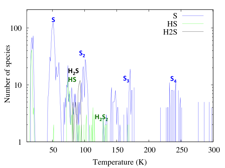
Figure 8: TPD from Monte Carlo simulations of H₂S. In these simulations, shielding of molecules within the ice is not considered.The deposition rate of H₂S is 1ML/s, the heating ramp is 1K/min and G₀=5$\times$ 10⁶.

4.4.3 TPD simulations of irradiated H₂S: case with self shielding

We perform similar simulations than in the previous section but this time, considering that molecules shield themselves from the UV radiation. For simplicity, we consider that if a species is under another one, then it is shielded from radiation and will not receive photons. It is then expected that the layers under the surface will remain H₂S as long as they are covered by other species, and will then be exposed only when the layers above sublimate. The results are presented in Figure 9. The surface coverage is shown from temperatures of 8 K (top left panel), 50 K (top middle panel), 100 K (top right panel) and 150 K (bottom left panel). These figures clearly show that there are much fewer chains on the surface than when shielded is not considered, as in Figure 8, and that instead species such as H₂S₂ (2 green boxes attached together) or H₂S₃ (1 blue box surrounded by 2 green boxes), are formed on the surface. However, no chains longer than S₃ are created, which is shown in Figure 9 bottom left panel, when chains are highlighted in different colors (for a surface temperature of 150 K). Therefore, there is no species on the surface after $\sim$ 180 K as the binding energies of these chains are too low. This is reflected by the TPD in Figure 10. This figure shows that S-chains are present, but only containing 2 to 3 sulfur atoms. On the other hand, many hydrogenated sulfur species are present, desorbing at temperatures lower than 180 K.

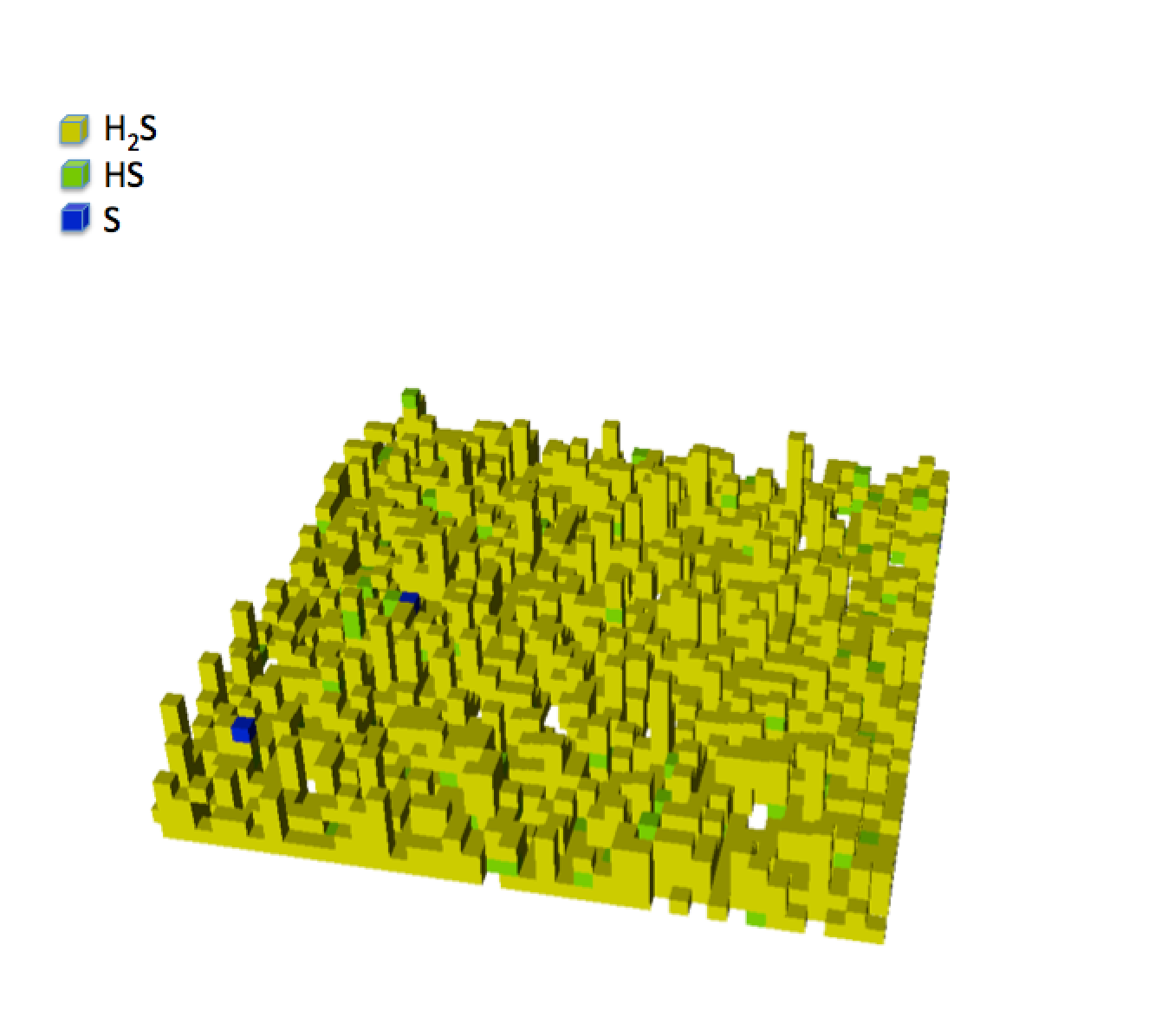
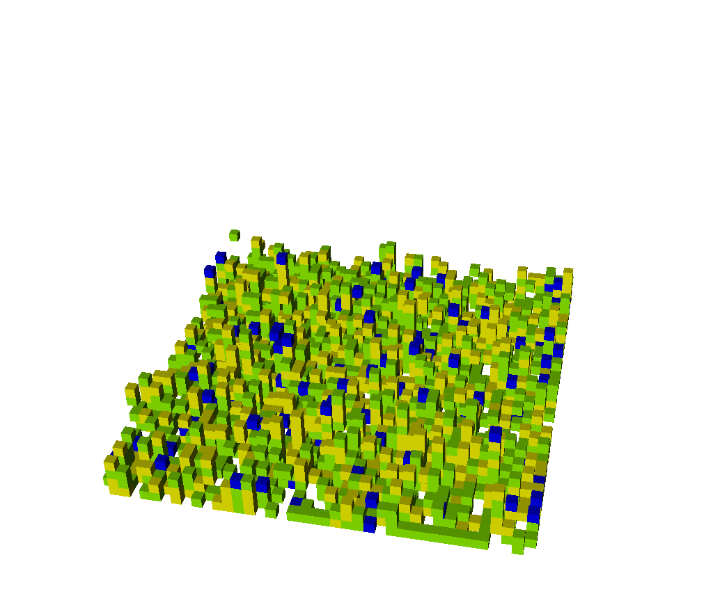
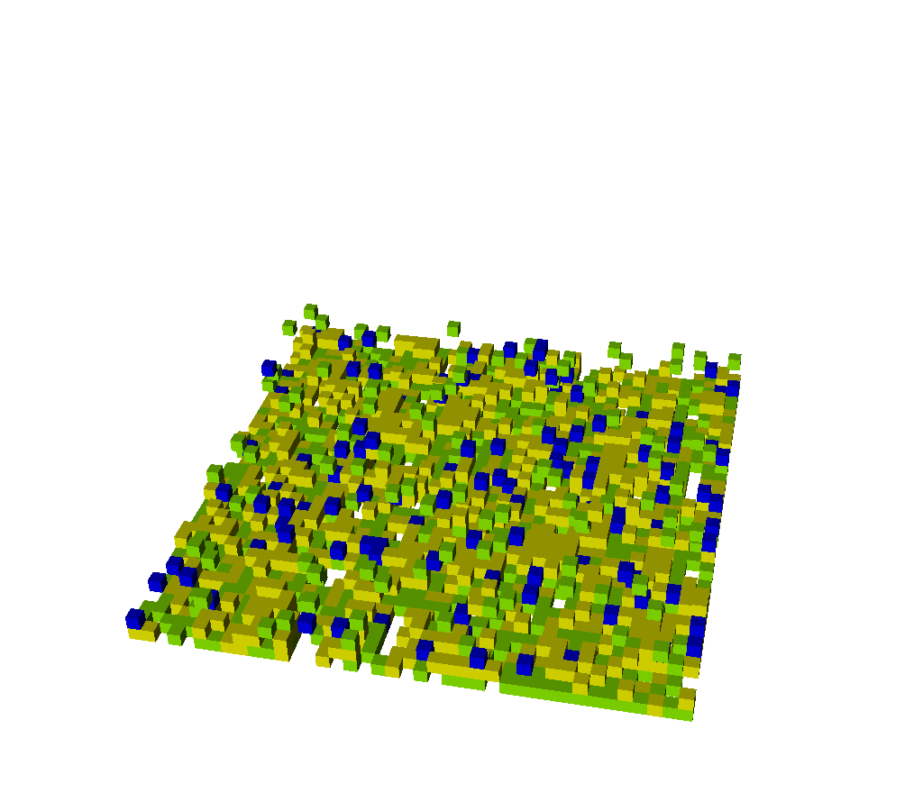
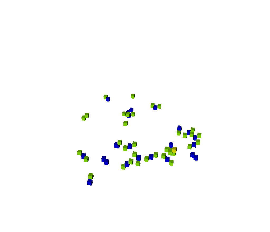
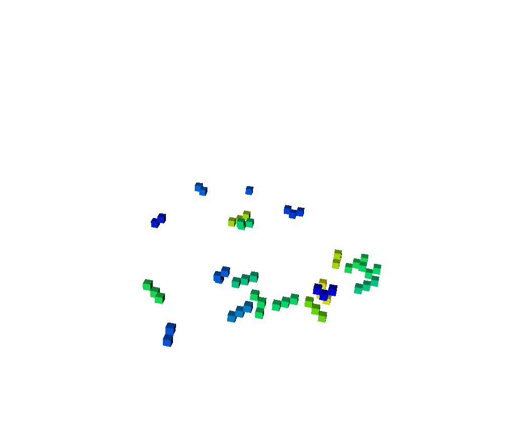
Figure 9: H₂S on the surface after deposition at 8 K (top left) and during TPD at 50 K (top middle), at 100 K, (top right), at 150 K (bottom left).The bottom right panel also shows the surface at 150 K but with the chains being highlighted by using one color per chain.In these simulations, the molecules in the ice do shield each other and photons cannot dissociate molecules if they are under another molecule. The deposition rate of H₂S is 1ML/s, the heating ramp is 1K/min and G₀=5$\times$ 10⁶.

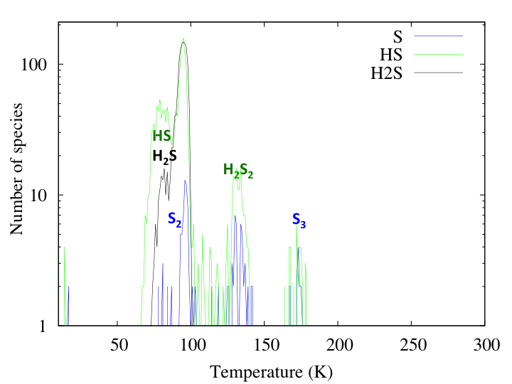
Figure 10: TPD from Monte Carlo simulations of H₂S. In these simulations, the molecules in the ice can shield each other. The deposition rate of H₂S is 1ML/s, the heating ramp is 1K/min and G₀=5$\times$ 10⁶.

5 Photo-processes in H₂S ice

In our simulations, we considered at first that icy molecules are not shielding each other from photons. As a result, we obtained a TPD dominated by atomic sulfur as well as S-chains, showing the presence of S-chains up to S₄ and a small amount of hydrogenated sulfur species. Our results show that residues are present on the surface at the end of the TPD, and that these residues are under the form of chains containing up to 6-7 sulfur atoms. Such TPD is reported in figure 7. We also considered in a second step that icy species could shield each other from UV photons, and obtained a different TPD, dominated by hydrogenated sulfur species, as shown in Figure 9. In this case, the species on the surface desorb below 200 K and no residue is found after the TPD.
The experimental results reported in Figure 5 show that the irradiation of H₂S ice allows for the formation of hydrogenated sulfur species which are dominating the TPD. The S-chains are also present and are desorbing until very high temperatures. These results are reproduced by our simulations if icy species can shield each other (hydrogenated sulfur species dominate the TPD) but also if icy species do not shield each other (S-chains up to 4 S atoms in the TPD, residue on the surface after the TPD). The experimental results shows that residues are still present on the surface after the TPD. Therefore, we can assume that H₂S species have a small shielding properties so that hydrogenated species can survive under the present experimental conditions, and S-chains can be formed.
Note that we do not consider in this study the effect of photodesorption or chemical desorption. Photodesorption will reduce the amount of solid H₂S, meaning that less H₂S is available for photo-dissociation to form HS, HS₂ and H₂S₂ as well as chains. This implies that the total number of ice species could differ. However, the fraction of H₂S versus other molecules should remain similar. Chemical desorption, on the other hand, would remove some formed species and send them into the gas phase (especially via H+HS $\rightarrow$ H₂S Oba et al. (2018); Shingledecker et al. (2020)). This will reduce the amount of H₂S species compared to other chemical species in the solid phase. Our present study aims at reproducing general experimental trends in the TPDs, so neglecting these processes will only slightly affect the abundances of the species in the ices which will not affect our conclusions.

6 Application to molecular clouds: sulfur depletion

Only $\sim$10 % of the currently detected molecules contain sulfur atoms. This apparent lack of chemical diversity in sulfur-bearing species is somewhat reflective of a great problem in astrochemistry: while the observed gaseous sulfur accounts for its total cosmic abundance (S/H$\sim$1.5$\times$10^-5) in diffuse clouds, there is an unexpected paucity of sulfur bearing molecules within molecular clouds. Indeed, the sum of the observed gas phase abundances of S-bearing molecules (mainly SO, SO₂, H₂S, and CS) constitute only ¡1 % of the cosmic abundance in cold and dense cores (n(H₂) $>$ 10⁴ cm^-3) (see, e.g., Agúndez & Wakelam, 2013). One could think that most of the sulfur is locked on the icy grain mantles in these regions but, surprisingly, the abundances of S-bearing species in the ice as measured by near-IR observations could only account for $<$ 5% of the total sulfur (Geballe et al., 1985; Palumbo et al., 1995; Boogert et al., 1997; Jiménez-Escobar & Muñoz Caro, 2011). Fuente et al. (2019) investigated the sulfur content in the translucent part of TMC 1 where the freeze-out of molecules on the grain surfaces is expected to be negligible. These observations revealed that gas-phase sulfur is already one order of magnitude lower than the cosmic value in translucent gas, i.e., 90% of S atoms incorporate to the solid grains in the transition between the diffuse medium and the translucent cloud, corresponding to an abundance of S in the gas $\sim$8 10^-7 (Fuente et al., 2019). sulfur atoms impinging in interstellar ice mantles are expected to form H₂S preferentially. The understanding of H₂S chemistry is therefore linked to the sulfur depletion problem. Chemical desorption of H₂S upon formation from HS + H is significant (Oba et al., 2018). Navarro-Almaida et al. (2020) investigated the H₂S abundance at the cloud edges and concluded that chemical desorption of H₂S from bare grains is needed to explain the high H₂S abundance observed in the translucent gas (n(H₂) $<$ 10⁴ cm^-3) towards TMC 1 and Barnard 1b.
In the present study we concentrate on the fraction of S atoms locked onto dust particles in the translucent phase, and therefore follow the fate of S atoms impinging the dust under these conditions. We can then address whether the high depletion of sulfur could be explained by our models and more specifically, could be under the form of sulfur chains or HS or H₂S. In translucent clouds, sulfur is mainly under the form of S⁺ (Laas & Caselli, 2019) and in dense PDRs S⁺ can be present until extinction of $\sim$4 (for PDRs with n_H=10⁶ cm^-3 and $\chi$=2 10⁵, see Sternberg & Dalgarno 1995). The fact that sulfur is under cationic form influences its accretion rates, as discussed in Ruffle et al. (1999). We therefore adopt a correction factor of 1+$\frac{167}{T}$ to account for the fact that the accretion rates are increased due to the charges of the sulfur as mentioned in Ruffle et al. (1999). We performed simulations for translucent cloud conditions taking into account the fact that the accretion rate of S⁺ is higher due to the effect of the charge. The conditions we used in our simulations are reported in Table 5 and are taken from Laas & Caselli (2019) and Snow & McCall (2006). In these simulations, reported in the left panel of Figure 11, we show the coverage of S compared to HS and H₂S as a function of time in translucent cloud conditions. The figure shows the increase of atomic sulfur under the form of S chains compared to H₂S and HS. The fact that S forms chains preferentially compared to HS or H₂S comes from the fact that in the gas phase, the ratio between atomic hydrogen and sulfur is 20 (see conditions in table 5). However, due to the fact that sulfur is under cationic form, its accretion rate is increased by 1+167/T which implies an accretion rate 7.5 times faster. This means that for each S⁺ accreting on the dust, 3 H atoms accrete. At temperatures of 17K, the residence time of H atoms is very short, and therefore S atoms can make S chains. These chains are not due to diffusion but to the fact that S⁺ arrive on an adsorbed S atom (or a S-chain) and makes a (larger) chain.  In order to address whether the sulfur adsorbed on the dust surface could be responsible for the depletion of sulfur in the gas phase, we estimate how much gas phase sulfur is needed to obtain the coverage obtained in our simulations. The surface area represented by carbon dust is n_c$\times$ $\sigma_{c}$ = 7.2 10^-22 cm^-1, by silicate dust is n_s$\times$ $\sigma_{s}$ = 4.4 10^-21 cm^-1, and by PAHs is $\sigma_{c}$ = 3.4 10^-21 cm^-1 (Weingartner & Draine (2001); we consider the possibility for S-chains to form on PAHs). This corresponds to a total area of 8.5 10^-21 cm^-1. This total area is multiplied by the number of sites per area (10¹⁵ cm^-2) to obtain the number density of sites per cm³ which is 8.5 10^-6 cm^-3. This implies that if the grains would be covered by one monolayer of S (or HS or H₂S), then 8.5 10^-6 S atoms would be missing from the gas phase and the gas phase density of sulfur would drop to 1.4 10^-6. The abundances of sulfur in translucent clouds have been reported to be $\sim$ 8 10^-7 (this is the most likely value taking into account the uncertainties 0.4-2.2 10^-6; Fuente et al. 2019) . Looking at our results, we show that such depletion of sulfur can occur in few times $\sim$10⁴ years. We therefore suggest that the sulfur under the form of S⁺ in translucent clouds plays a significant role in setting the S depletion in denser regions, as the timescales to reach such depletion are quite short. The fact that sulfur atoms are creating chains on the surface allows for layers to be built that can represent more than 100$\%$ surface coverage. The increase in S on the surface is due to the formation of S-chains. The right panel of Figure 11 shows the surface coverage at the end of the simulations, the blue boxes showing the sulfur atoms and how they are organized on the surface. Our simulations suggest the creation of long S-chains under translucent cloud conditions which can explain the important depletion observed in the gas phase. As translucent clouds evolved further to molecular clouds and dense cores phases, and extinction increases, these S-rich grains will then be covered with ices. Some of these ices is composed of H₂S which will adsorb on the icy grains during these phases as a fraction of sulfur is still in the gas phase. The sulfur chains from the translucent cloud phase, buried underneath the ice, cannot desorb in the hot core or hot corinos phases since the temperature of the dust in these environments is too small to allow desorption (we observe up to S₄ until 300 K). These buried chains could be ejected again in the gas phase upon shocks that would vaporize the ice, dust and these chains. These chains could also be observed in our solar system within Interplanetary dust particles (IDPs), meteorites and comets under a refractory form.

nH	nHI/nH a	nS+/nH	Tgas (K)	Tdust (K)	AV
5 103	2 10-4	10-5	25	17	1.6

Table 5: Parameters used in our simulations for translucent clouds conditions. Taken from Laas & Caselli (2019); ^a taken from Cazaux & Spaans (2009).

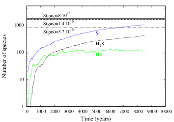
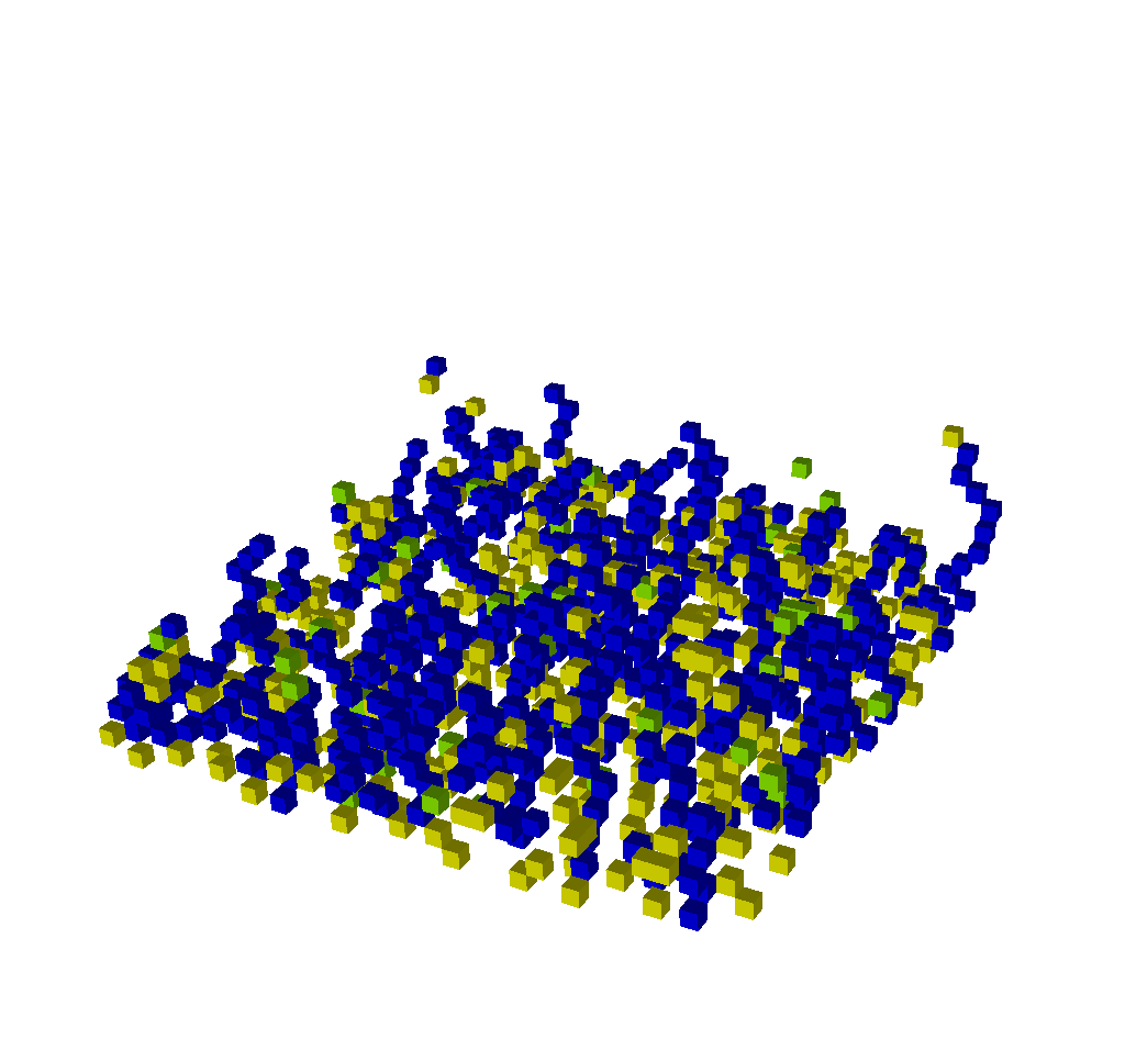
Figure 11: Sulfur coverage of S, HS or H₂ S as a function of time for translucent cloud models with increase of accretion rate due to the charge (left panel). The composition of the surface is visualised (right panel). In these simulations, the temperature of the dust is 17K, and G₀=1.

7 Application to solar system conditions: origin of sulfur found in cometary material

In the present study, we show that UV irradiation of H₂S ice results in the formation of S chains. These chains are increasingly resistant to UV as their size increase. We show that H₂S species in the ice can shield other sulfur bearing species to some extent. Our study therefore shows that photo-processes of H₂S ices can lead to the formation of S chains that either desorb (below 250 K for chains up to S₄) or stay on the surface as residue for chains with more than 4 sulfur atoms.
Comets are known to be rich in H₂S ice representing $\sim$56% of the total sulfur budget, with some minor contribution from SO₂, SO and S₂ (0.14%, Calmonte et al., 2016). The abundance of H₂S in comets is up to 1.5$\%$ relative to H₂O as inferred from millimeter and submillimeter observations (Bockelée-Morvan et al., 2000; Boissier et al., 2007). In comet 67P, data analysis from Rosina (Rosetta Orbiter Spectrometer for Ion and Neutral Analysis) showed the presence of S₃ and S₄. Calmonte et al. (2016) discussed whether these are real parent molecules or the products of even heavier S_n, fragmenting into S₃ and S₄. In the present study, we show that large S_n do not desorb at temperatures below 300 K (experimental temperature range in the TPD), but stay as residue in the ice. We therefore suggest that the S₃ and S₄ chains measured in cometary material do not come from fragmentation from large S_n, but from UV processing of H₂S bearing-ices leading to small sulfur chains.

The detection of S₂, S₃ and S₄ makes radiolysis of H₂S a very likely formation process, as already discussed by other authors (Grim & Greenberg 1987; Jiménez-Escobar et al. 2012; Woods et al. 2015) which could well connect the cometary ice to the ISM. In particular, the S₂/H₂S abundance ratio in comet 67P varied from less than 1% to about 3.4% (Calmonte et al., 2016), the latter value requires a substantial UV dose to convert H₂S into S₂ in the ice (Jiménez-Escobar et al., 2012). Other species, such as H₂S₂ and S₂H, that are efficiently formed in H₂S ice irradiation experiments (Jiménez-Escobar et al., 2012, this work), could not be detected in the coma of 67P; this was probably due to overlap with other species of similar mass-to-charge ratio (Calmonte et al., 2016). The present study suggests that small sulfur chains come either from UV photo-processes of H₂S or from S depletion in the cloud prior to the formation of the protosun. The different environments at which the formation of these S-chains occur are illustrated in figure 12. In the translucent stage, S-chains are formed on bare grains due to the accretion of cationic S on grain surfaces, while in dense clouds, S-chains are formed via UV photo-processes of H₂S ice. In this case, these chains are within the ices Therefore, observation of small S chains alone cannot allow distinguishing between the two possible formation scenarios. Large chains, produced in the second scenario (translucent cloud phase), are present in the residues within and/or beneath ice mantles that do not desorb at temperatures typical of cometary conditions, and are therefore impossible to observe in the gas phase. Infrared bands are expected for the S_n species that would be very difficult to detect since they will be masked by the intense absorption features of ice species in the same spectral region. In particular, S₈ displays a band near 465 cm^-1 and other bands in the far-IR (Trofimov et al., 2009). These species could have been detected by the COSAC-Rosetta instrument on board the Philae lander, but the non-nominal landing on 67P comet nucleus did not allow to extract a sample for analysis (Goesmann et al. (2015). Looking at the present experiments and simulations, UV photolysis of H₂S ices produces a fraction of H₂S/S_n (with n $\leq$3) of the order of 10² (from Fig. 5), while the S_n built in the translucent cloud conditions has mainly n $>$ 4. The observations of S-chains in comet 67P seem to be related with UV processes of H₂S ice, rather than S-chains originating from the translucent cloud phase. This is in agreement with Calmonte et al. (2016) suggesting an ice origin of the S-chains. Comparison of the different periods in the evolution of 67P show that at least in 2 periods the S follows more or less the H₂S abundances, suggesting a common origin in the ice matrix.

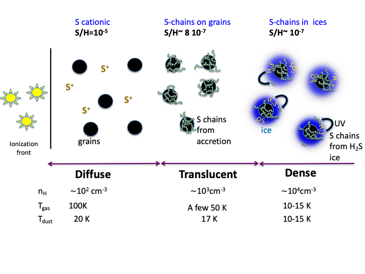
Figure 12: Sketch summarizing the results for the formation of S-chains via accretion in the translucent cloud phase, and via UV photo-processes of H₂S ices in molecular cloud phase. Adapted from Fuente et al. (2019).

8 Conclusions

1. The 2538 cm^-1 band profile (H-S stretching) and integrated band strength of H₂S ice change gradually up to about 60 K. Above this temperature the structure is dominated by the crystalline phase, as evidenced by the distinctive narrow features of antisymmetric and symmetric S-H modes, see Fig. 1.

2. Upon H₂S irradiation, the efficient formation of H₂S₂ molecules occurs already at 8 K, the lowest temperature in our experiments. Above 100 K, H₂S ice sublimates and H₂S₂ molecules are allowed to form a crystalline ice structure, see Fig. 2. H₂S₂ desorbs around 144 K.

3. Molecules H₂S_x with $x$ ¿ 2 are also observed in the IR, Fig. 3. This is confirmed by the desorption of H₂S₃ during warm-up near 184 K, while H₂S₄ desorbs near 204 K, see Fig. 4.

4. During warm-up of the previously irradiated H₂S ice, the more volatile S_x species are detected. S desorbs near 58 K, S₂ desorbs around 113 K, and S₄ desorbs at 283 K, see Fig. 5. Larger S_x species are more refractory and remain on the substrate at room temperature, being S₈ by far the most abundant species in these residues (Muñoz Caro, 2003).

5. Monte Carlo simulations of the photo-dissociation of H₂S ice shows that hydrogenated sulfur species observed in the experiments could be reproduced if species in the ice can shield each other. However, this shielding should be not too efficient to be able to reproduce the S-chains observed in the experiments. We predict that the residues remaining after the TPD in the experiments are S-chains with a length up to 6-7 S atoms.

6. Applying our Monte Carlo simulations to translucent clouds conditions, we show that long S-chains are created in a rather short timescales of few 10⁴ years. The important depletion observed in these environments can therefore be explained by grains covered by S_n. These grains will be buried under ices in later stages as the cloud evolves.

7. Small S-chains observed in comets could in theory originate from processed H₂S ices (from molecular cloud phases) or from S-chains from the translucent cloud phase. Since small chains are being mainly produced by photo-processes of H₂S ice, we suggest that observations of S₃ and S₄ in 67P have an icy origin, and are not due to processes of long chains from the translucent cloud phase.