The Chen–Yang volume conjecture for knots in handlebodies

Abstract.

In 2015, Chen and Yang proposed a volume conjecture that stated that certain Turaev–Viro invariants of an hyperbolic $3$-manifold should grow exponentially with a rate equal to the hyperbolic volume.

Since then, this conjecture has been proven or numerically tested for several hyperbolic $3$-manifolds, either closed or with boundary, the boundary being either a family of tori or a family of higher genus surfaces. The current paper now provides new numerical checks of this volume conjecture for $3$-manifolds with one toroidal boundary component and one geodesic boundary component.

More precisely, we study a family of hyperbolic $3$-manifolds $M_{g}$ introduced by Frigerio. Each $M_{g}$ can be seen as the complement of a knot in an handlebody of genus $g$.

We provide an explicit code that computes the Turaev–Viro invariants of these manifolds $M_{g}$, and we then numerically check the Chen–Yang volume conjecture for the first six members of this family.

Furthermore, we propose an extension of the volume conjecture, where the second coefficient of the asymptotic expansion only depends on the topology of the boundary of the manifold. We numerically check this property for the manifolds $M_{2},\ldots,M_{7}$ and we also observe that the second coefficient grows linearly in the Euler characteristic $\chi(\partial M_{g})$.

1. Introduction

Quantum topology began in 1984 with the definition of the Jones Polynomial [9]. Since then, several new invariants of knots and 3-manifolds were defined and, inspired by quantum field theories, the volume conjecture of Kashaev [10] and its variants rose to be among the most studied conjectures in quantum topology. What is intriguing about these volume conjectures is that they link quantum invariants of manifolds to the hyperbolic structure of these manifolds. In [3], Chen–Yang proposed a volume conjecture using a family $\left\{TV_{r,2}\right\}_{r\in\mathbb{N}_{\geq 3}}$ of Turaev-Viro type invariants for compact 3-manifolds.

Conjecture 1.1 (Conjecture 1.1, [3], Chen-Yang).

Let $M$ be a compact hyperbolic 3-manifold. Then for $r$ running over all odd integers such that $r\geq 3$,

$$\lim_{r\to\infty}\frac{2\pi}{r-2}\log\left(TV_{r,2}(M)\right)=\mathrm{Vol}(M),$$

where $\mathrm{Vol}(M)$ is the hyperbolic volume of $M$.

This conjecture has since then been proven [4, 13, 16] or numerically tested [3, 12] for several hyperbolic $3$-manifolds, mostly for manifolds without boundary, but also manifolds with toroidal boundary and manifolds with totally geodesic boundary of genus $g\geq 2$. However, there is currently no test of this conjecture for an hyperbolic $3$-manifold with a boundary which has both a toroidal component and a totally geodesic boundary component of genus $g\geq 2$. In this paper, we thus propose to test the Chen–Yang volume conjecture for a family of $3$-manifolds $\left\{M_{g}\right\}_{g\in\mathbb{N}_{\geq 2}}$, each $M_{g}$ being the exterior of a knot in a handlebody of genus $g$. These manifolds were constructed and studied by Frigerio [5].

We will actually go one step further, as we will test an extension of Conjecture 1.1 stated as follows:

Conjecture 1.2.

Let $M$ be a compact hyperbolic 3-manifold of volume $\mathrm{Vol}(M)$. Then for $r$ running over all odd integers such that $r\geq 3$,

$$TV_{r,2}(M)\underset{r\to\infty}{\sim}\omega\cdot r^{b}\cdot e^{\frac{\mathrm{Vol}(M)}{2\pi}(r-2)}\cdot\left(1+O\left(\frac{1}{r-2}\right)\right),$$

where $\omega,b\in\mathbb{R}$ are independent of $r$, or equivalently,

$$\frac{2\pi}{r-2}\log\left(TV_{r,2}(M)\right)\underset{r\to\infty}{\sim}\mathrm{Vol}(M)+b\dfrac{2\pi\ln(r-2)}{r-2}+c\dfrac{1}{r-2}+O\left(\frac{1}{(r-2)^{2}}\right),$$

where $b\in\mathbb{R}$ and $c\in\mathbb{C}$ are independent of $r$.

Variants of Conjecture 1.2 have been previously stated, proven and numerically checked, notably by Chen–Yang [2, Section 6] (for some manifolds with boundary), and by Ohtsuki [13] and Gang-Romo-Yamasaki [6] (for certain closed manifolds, via the usual quadratic relation between Reshetikhin–Turaev invariants and Turaev–Viro invariants). In the present paper, we aim to numerically test Conjecture 1.2 for Frigerio’s manifolds $M_{g}$.

A yet stronger conjecture surmises that the coefficient $b$ in Conjecture 1.2 should only depend on the topology of the boundary $\partial M$. We go further and conjecture that $b$ is linear in $\chi(\partial M)$, as stated as follows:

Conjecture 1.3.

Let $\mathcal{M}$ be the set of compact hyperbolic 3-manifolds for which Conjecture 1.2 holds. Then, for all $M\in\mathcal{M}$, the coefficient $b(M)$ in Conjecture 1.2 only depends on the topology of $\partial M$, as an affine function of the Euler characteristic $\chi(\partial M)$.

Conjecture 1.3, as stated here, might be too strong to be true. Nevertheless, in this paper, it follows from numerical computations that Conjecture 1.3 appears to hold for Frigerio’s manifolds $M_{g}$.

After reviewing preliminaries about triangulations, hyperbolic volumes, colorings of triangulations and Turaev–Viro invariants in Section 3, we discuss the manifolds $M_{g}$ in Section 4: in particular we describe their ideal triangulations $\mathcal{T}_{g}$, constructed by Frigerio. We observe that these ideal triangulations admit an ordered structure, which means we can orient all edges in a coherent way with face gluings and such that no triangle admits a cycle.

Proposition 1.4 (Proposition 4.3).

The triangulations $\mathcal{T}_{g}$ of the manifolds $M_{g}$ admit an ordered structure.

This property will not be used for the rest of the paper, but may be useful in the future for studying other quantum invariants which are only defined on ordered triangulations [1, 11], in the specific cases of these manifolds $M_{g}$.

For two fixed integers $r\geqslant 3$ and $s\geqslant 1$, the Turaev-Viro invariant $TV_{r,s}(M,\mathcal{T})$ of a triangulated manifold $(M,\mathcal{T})$ is defined as a sum over a (usually large) set of admissible colorings of the triangulation $\mathcal{T}$. Hence, in order to compute the Turaev-Viro invariants $TV_{r,s}(M_{g},\mathcal{T}_{g})$, we first need to describe the associated set of admissible colorings $\mathcal{A}_{r}(M_{g},\mathcal{T}_{g})$. The main theorem of this paper provides a description of $\mathcal{A}_{r}(M_{g},\mathcal{T}_{g})$ that is both clearer than the original definition and easier to transform into computer code (in Section 5.2). We now phrase it without technical details:

Theorem 1.5 (Theorem 4.8).

An admissible coloring of $\mathcal{T}_{g}$ has to satisfy a certain set of admissibility conditions, which are equivalent to another explicit and more convenient set of conditions.

The proof of Theorem 1.5 is quite lengthy but can give insights on how to simplify admissibility conditions for other examples of triangulations. The new set of conditions given by Theorem 1.5 will be used later on in Section 5.2.

In Section 6, we study the specific cases of $(M_{g},\mathcal{T}_{g})$ for $2\leqslant g\leqslant 7$. We numerically compute their hyperbolic volume (thanks to results of Frigerio [5] and Ushijima [15]) and their logarithmic Turaev–Viro invariants $QV_{r,2}(M_{g}):=\frac{2\pi}{r-2}\log(TV_{r,2}(M_{g},\mathcal{T}_{g}))$ for several values of $r$. For increasing values of $r$, we observe a convergence as expected in Conjecture 1.1 (for $2\leqslant g\leqslant 7$), and then a surprising pattern break for $g\in\{2,3\}$.

Numerical test 1.6 (Sections 6.1.4, 6.2.4 and 6.3).

Conjectures 1.1 and 1.2 appear to hold numerically for the manifolds $M_{2},\ldots,M_{7}$, barring possible numerical errors for $M_{2}$ and $M_{3}$.

More precisely, the graph of the function $QV_{r,2}(M_{2})$ (resp. $QV_{r,2}(M_{3})$) shows a converging behavior up to $r=33$ (resp. $r=31$) and an unexpected increase after $r=33$ (resp. $r=31$). The graph of the function $QV_{r,2}(M_{g})$ (for $4\leqslant g\leqslant 7$) shows a converging behavior.

We offer hypotheses to explain the previous pattern breaks, and we furthermore compute an interpolating function for the data, which not only fits the pre-break values quite well, but also provides a promising candidate for the next term $b$ in the expected asymptotic expansion of $QV_{r,2}(M_{g})$ (see Conjecture 1.2).

In Section 5 we provide our entire code (written in SageMath), with annotations for clarity. In particular, we program functions that compute the hyperbolic volumes and Turaev–Viro invariants for the manifolds $M_{g}$, and we list several of these values in the tables of Figures 9 and 10.

Finally, we observe a linear behavior for the second coefficient $b$, as expected in Conjecture 1.3.

Numerical test 1.7 (Section 6.4).

Conjecture 1.3 appears to hold numerically for the manifolds $M_{2},\ldots,M_{7}$.

The results in this article follow in part from the Master’s thesis [7] of the second author.

2. Materials and methods

All the calculations were performed on SageMath (a free open-source mathematics software system using Python 3), on a computer equipped with a Intel® Core™ i5-8500 CPU @ 3.00GHz × 6 processor.

3. Preliminaries

3.1. Ideal triangulations

In this section, we follow some conventions of [3] and [15]. A pseudo $3$-manifold is a topological space $M$ such that each point $p$ of $M$ has an (open) neighborhood $U_{p}$ that is homeomorphic to a cone over a surface. A triangulation $\mathcal{T}$ of a pseudo $3$-manifold $M$ consists of a disjoint union $T_{1}\sqcup\ldots\sqcup T_{N}$ of finitely many Euclidean tetrahedra and of a collection of affine homeomorphisms between pairs of faces in $T_{1}\sqcup\ldots\sqcup T_{N}$ such that the quotient space $\left(T_{1}\sqcup\ldots\sqcup T_{N}\right)/\sim$ is homeomorphic to $M$. For $i\in\{0,1,2,3\}$, we denote $\mathcal{T}^{i}$ (resp. $\mathcal{T}^{i,\sim}$) the $i$-skeleton of the disjoint union of tetrahedra in $\mathcal{T}$ (resp. the $i$-skeleton of the quotient space homeomorphic to $M$). We say that an element $\nu$ of the set $\mathcal{T}^{0,\sim}$ of vertices of $M$ is regular (resp. ideal, hyperideal) if its associated neighborhood $U_{\nu}$ is a cone over a sphere (resp. over a torus, over a surface of genus at least $2$). Finally, we say that a compact $3$-manifold $N$ with boundary admits an ideal triangulation $\mathcal{T}$ if no vertices in $\mathcal{T}^{0,\sim}$ are regular, and $N$ is obtained from the quotient space of $\mathcal{T}$ by removing open neighborhoods $U_{\nu}$ of all vertices $\nu$ in $\mathcal{T}^{0,\sim}$.

3.2. Hyperbolic volume

In [15], Ushijima gives a volume formula for a generalized hyperbolic tetrahedron with a given angle structure. Let us detail this formula and its components. Let $T=T(A,B,C,D,E,F)$ be a generalized tetrahedron in the hyperbolic space $\mathbb{H}^{3}$ whose angle structure is as in Figure 1 ($A,\ldots,F\in[0,\pi]$ are dihedral angles).

Figure 1. The configuration of dihedral angles on $T$.

Let $G$ denote the associated Gram matrix:

$$G=\left(\begin{array}[]{cccc}1&-\cos\,A&-\cos\,B&-\cos\,F\\ -\cos\,A&1&-\cos\,C&-\cos\,E\\ -\cos\,B&-\cos\,C&1&-\cos\,D\\ -\cos\,F&-\cos\,E&-\cos\,D&1\end{array}\right).$$

Let $\mathrm{Li_{2}}(z)$ be the dilogarithm function defined for $z\in\mathbb{C}\setminus[1,\infty)$ in [15, Introduction] by the analytic continuation of the following integral:

$$\mathrm{Li_{2}}(x):=-\int_{0}^{x}\frac{\log(1-t)}{t}\text{d}t\quad\text{for }x\in\mathbb{R}_{>0}.$$

Let $I$ be the principal square root of $-1$ , $a:=\exp(I\cdot A)$, $b:=\exp(I\cdot B)$, …, $f:=\exp(I\cdot F)$ and let $U(z,T)$ be the complex valued function defined as follows:

$$U(z,T):=\frac{1}{2}( \mathrm{Li_{2}}(z)+\mathrm{Li_{2}}(abdez)+\mathrm{Li_{2}}(acdfz)+\mathrm{Li_{2}}(bcefz)$$

$$-\mathrm{Li_{2}}(-abcz)-\mathrm{Li_{2}}(-aefz)-\mathrm{Li_{2}}(-bdfz)-\mathrm{Li_{2}}(-cdez)).$$

We denote by $z_{+}$ and $z_{-}$ the two complex numbers defined as follows:

$$z_{\pm}:= -2\frac{\sin\,A\sin\,D+\sin\,B\sin\,E+\sin\,C\sin\,F\pm\sqrt{\text{det}\,G}}{ad+be+cf+abf+ace+bcd+def+abcdef},$$

where $\sqrt{\text{det}\,G}\in I\mathbb{R}_{>0}$ is the principal square root of $\text{det}\,G$.

Proposition 3.1 (Ushijima, [15] Theorem 1.1).

The hyperbolic volume $\mathrm{Vol}(T)$ of a generalized tetrahedron $T=T(A,B,C,D,E,F)$ is given as follows:

$$\mathrm{Vol}(T)=\frac{1}{2}\mathcal{I}(U(z_{-},T)-U(z_{+},T)),$$

where $\mathcal{I}$ means the imaginary part.

In Section 5.1.1 we provide a code to compute the previous functions and formula.

3.3. Admissible colorings

We will mostly follow the notations, conventions and definitions of [3, Section 2]. For the remainder of this paper, let us fix a pair $(r,s)\in\mathbb{N}^{2}$ such that $r\geq 3$ and $s\geq 1$. We will only specify $s=2$ when studying the Chen–Yang volume conjecture.

Notation 3.2.

Let $\frac{\mathbb{N}}{2}=\left\{0,\frac{1}{2},1,\frac{3}{2},...\right\}$ denote the set of non-negative half-integers. Let $\frac{\mathbb{N}_{odd}}{2}=\left\{\frac{1}{2},\frac{3}{2},\frac{5}{2},...\right\}$ denote the set of non-negative half-odd-integers. Let $I_{r}$ denote the subset $\left\{0,\frac{1}{2},1,...,\frac{r-2}{2}\right\}$ of $\frac{\mathbb{N}}{2}$.

As a convention, we let $\sqrt{-x}=I\sqrt{x}$ for $x\geq 0$.

Definition 3.3.

A triple $(i,j,k)$ of elements of $I_{r}$ is called admissible if it satisfies the following conditions:

1. 1. $i+j\geq k$,

   2. $j+k\geq i$,

   3. $k+i\geq j$,

2. $i+j+k\in\mathbb{N}$,

3. $i+j+k\leq r\scalebox{1.8}[1.0]{-}2$.

Definition 3.4.

Let $M$ be an hyperbolic compact 3-manifold with boundary that admits an ideal triangulation $\mathcal{T}$. A coloring at level r of $(M,\mathcal{T})$ is an application $c:\mathcal{T}^{1,\sim}\to I_{r}$. The coloring is called admissible if for every $T\in\mathcal{T}^{3}$, the triples $\left(c([e_{01}]),c([e_{02}]),c([e_{03}])\right)$, $\left(c([e_{01}]),c([e_{12}]),c([e_{13}])\right)$, $\left(c([e_{02}]),c([e_{12}]),c([e_{23}])\right)$ and $\left(c([e_{03}]),c([e_{13}]),c([e_{23}])\right)$ are admissible, where $[e_{kl}]\in\mathcal{T}^{1,\sim}$ denotes the equivalence class under $\sim$ of the edge $e_{kl}$ of $T$ (for $k,l\in\{0,1,2,3\}$ such that $k\neq l$).

3.4. Turaev–Viro invariants

Recall that $r,s\in\mathbb{N}$ are such that $r\geq 3$ and $s\geq 1$.

For $n\in\mathbb{N}$, the quantum number $[n]$ is the real number defined by

$$[n]:=\frac{\sin\left(\frac{ns\pi}{r}\right)}{\sin\left(\frac{s\pi}{r}\right)}\in\mathbb{R}.$$

For $n\in\mathbb{N}$, the quantum factorial $[n]!$ is defined by

$$[n]!:=[n][n\scalebox{1.8}[1.0]{-}1]...[2][1]\in\mathbb{R},$$

and, as a convention, $[0]!=1$. For an admissible triple $(i,j,k)\in(I_{r})^{3}$, we define

$$\Delta(i,j,k):=\sqrt{\frac{[i+j\scalebox{1.8}[1.0]{-}k]![i\scalebox{1.8}[1.0]{-}j+k]![\scalebox{1.8}[1.0]{-}i+j+k]!}{[i+j+k+1]!}}.$$

Definition 3.5 (Quantum $6j$-symbols).

Let $(i,j,k,l,m,n)$ be a 6-tuple of elements of $I_{r}$ such that $(i,j,k)$, $(j,l,n)$, $(i,m,n)$ and $(k,l,m)$ are admissible.

Let $T_{1}=i+j+k$, $T_{2}=j+l+n$, $T_{3}=i+m+n$, $T_{4}=k+l+m$, $Q_{1}=i+j+l+m$, $Q_{2}=i+k+l+n$ and $Q_{3}=j+k+m+n$.

Then the quantum $6j$-symbol for the 6-tuple $(i,j,k,l,m,n)$ is defined by

$$\begin{vmatrix}i&j&k\\ l&m&n\end{vmatrix}:= \sqrt{\scalebox{1.8}[1.0]{-}1}^{-2(i+j+k+l+m+n)}\Delta(i,j,k)\Delta(j,l,n)\Delta(i,m,n)\Delta(k,l,m)$$

$$\cdot \sum_{z=\max\{T_{1},T_{2},T_{3},T_{4}\}}^{\min\{Q_{1},Q_{2},Q_{3}\}}\frac{(\scalebox{1.8}[1.0]{-}1)^{z}[z+1]!}{[z\scalebox{1.8}[1.0]{-}T_{1}]![z\scalebox{1.8}[1.0]{-}T_{2}]![z\scalebox{1.8}[1.0]{-}T_{3}]![z\scalebox{1.8}[1.0]{-}T_{4}]![Q_{1}\scalebox{1.8}[1.0]{-}z]![Q_{2}\scalebox{1.8}[1.0]{-}z]![Q_{3}\scalebox{1.8}[1.0]{-}z]!}.$$

Proposition 3.6 (Allowed symbol permutations).

Let $(i,j,k,l,m,n)$ be a 6-tuple of elements of $I_{r}$ such that $(i,j,k)$, $(j,l,n)$, $(i,m,n)$, $(k,l,m)$ are admissible.

Then, we have the following allowed permutations:

$$\begin{vmatrix}i&j&k\\ l&m&n\end{vmatrix}=\begin{vmatrix}j&i&k\\ m&l&n\end{vmatrix}=\begin{vmatrix}i&k&j\\ l&n&m\end{vmatrix}=\begin{vmatrix}i&m&n\\ l&j&k\end{vmatrix}=\begin{vmatrix}l&m&k\\ i&j&n\end{vmatrix}=\begin{vmatrix}l&j&n\\ i&m&k\end{vmatrix}.$$

Let $M$ be a pseudo-$3$-manifold that admits an triangulation $\mathcal{T}$. Let $R\subset\mathcal{T}^{0,\sim}$ denote the set of regular vertices. We define the regular vertices term as $N:=\left(\sum_{i\in I_{r}}w_{i}^{2}\right)^{-|R|}$. Let $c:\mathcal{T}^{1,\sim}\to I_{r}$ be an admissible coloring at level $r$ of $(M,\mathcal{T})$. For $\eta\in\mathcal{T}^{1,\sim}$, we define the edge term $|\eta|_{c}:=w_{c(\eta)}$, where $w_{i}:=(\scalebox{1.8}[1.0]{-}1)^{2i}[2i+1]$ for $i\in I_{r}$. For $T\in\mathcal{T}^{3}$, we define the tetrahedron term as

$$|T|_{c}=\begin{vmatrix}c([e_{01}])&c([e_{02}])&c([e_{12}])\\ c([e_{23}])&c([e_{13}])&c([e_{03}])\end{vmatrix},$$

where $[e_{kl}]\in\mathcal{T}^{1,\sim}$ denotes the equivalence class under $\sim$ of the edge $e_{kl}$ of $T$ (for $k,l\in\{0,1,2,3\}$ such that $k\neq l$).

Definition 3.7 (Turaev–Viro invariant).

Let $m=\left|\mathcal{T}^{1,\sim}\right|$. Let $\mathcal{A}_{r}(M,\mathcal{T}):=$

$$\left\{(c(\eta_{0}),...,c(\eta_{m}))\ |\ c:\mathcal{T}^{1,\sim}\to I_{r}\text{ is an admissible coloring at level }r\text{ of }(M,\mathcal{T})\right\}.$$

We define the Turaev–Viro invariant of $M$ as

$$TV_{r,s}(M,\mathcal{T}):=N\sum_{(c(\eta_{0}),...,c(\eta_{m}))\in\mathcal{A}_{r}(M,\mathcal{T})}\prod_{i=0}^{m}|\eta_{i}|_{c}\prod_{T\in X^{3}}|T|_{c}.$$

In [3, Theorem 2.6], Chen and Yang prove that the previously defined Turaev–Viro invariant of $M$ does not depend on the triangulation $\mathcal{T}$.

3.5. Volume conjecture

We can now state the Chen–Yang volume conjecture:

Conjecture 3.8 ([3], Conjecture 1.1).

Let $M$ be a compact hyperbolic 3-manifold. Then for $r$ running over all odd integers such that $r\geq 3$,

$$\lim_{r\to\infty}QV_{r,2}(M)=\lim_{r\to\infty}\frac{2\pi}{r-2}\log\left(TV_{r,2}(M)\right)=\mathrm{Vol}(M),$$

where $QV_{r,2}(M):=\frac{2\pi}{r-2}\log\left(TV_{r,2}(M)\right)$ and $\mathrm{Vol}(M)$ is the hyperbolic volume of $M$.

Remark 3.9.

In [2, Section 6.1], Chen and Yang discuss the potential asymptotic behavior of $QV_{r,2}(M)$ in more detail than in Conjecture 3.8. In particular, observations for specific $M$ with one boundary component lead them to ask if

$$QV_{r,2}(M)=\mathrm{Vol}(M)+b\dfrac{\ln(r-2)}{r-2}+c\dfrac{1}{r-2}+O\left(\dfrac{1}{(r-2)^{2}}\right),$$

where the numbers $b,c$ would depend only on $M$. In the examples they study, they find $b$ to be close to $\pi$ when $M$ has one toroidal boundary component and $-3\pi$ when $M$ has one geodesic boundary component of genus $2$. We rephrased this general question as Conjecture 1.2.

We will study in Sections 6.1.4 and 5.3 how likely these asymptotic behaviors seem for the manifolds $M_{2},M_{3},\ldots,M_{7}$ (which have two boundary components each, of different genera).

4. On Frigerio’s manifolds $M_{g}$

4.1. Frigerio’s construction

This section follows closely the construction in [5]. Let $g\in\mathbb{N}_{\geq 2}$. Let $S^{3}$ be the one point compactification of $\mathbb{R}^{3}$.

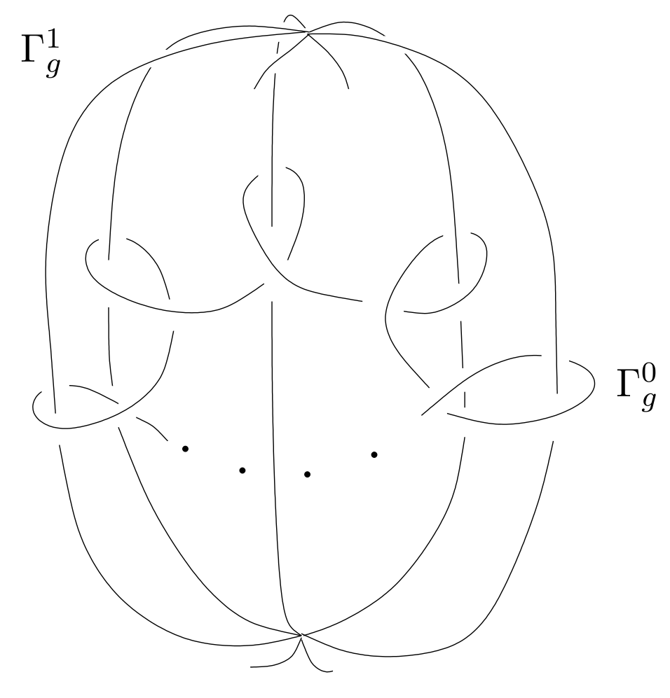
Figure 2. $\Gamma_{g}$ has two components: $\Gamma^{0}_{g}$ is a knot and $\Gamma^{1}_{g}$ is a graph with $g+1$ edges and two vertices. Source: [5, Figure 1]

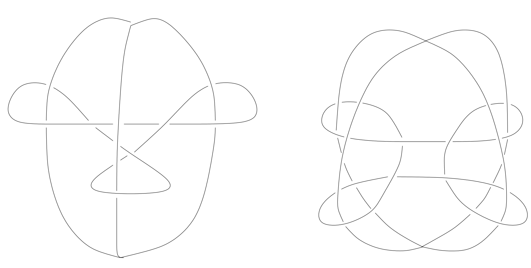
Figure 3. The graphs $\Gamma_{2}$ (on the left) and $\Gamma_{3}$ (on the right). Source: [5, Figure 2]

Let $\Gamma_{g}\subset S^{3}$ be the graph shown in Figure 2 (see Figure 3 for the cases $g=2$ and $g=3$). Let us denote by $\Gamma^{0}_{g}$ and $\Gamma^{1}_{g}$ the two connected components of $\Gamma_{g}$, where $\Gamma^{0}_{g}$ is a knot and $\Gamma^{1}_{g}$ has two vertices and $g+1$ edges. Let $U(\Gamma^{0}_{g})$ and $U(\Gamma^{1}_{g})$ denote open regular neighbourhoods of $\Gamma^{0}_{g}$ and $\Gamma^{1}_{g}$. Then $M_{g}$ is defined as the compact 3-manifold $M_{g}:=S^{3}\setminus\left\{U(\Gamma^{0}_{g}),U(\Gamma^{1}_{g})\right\}$ with boundary $\partial M=(\partial M)_{0}\cup(\partial M)_{1}$ such that $(\partial M)_{0}=\partial U(\Gamma^{0}_{g})\cong S^{1}\times S^{1}$ and $(\partial M)_{1}=\partial U(\Gamma^{1}_{g})\cong\Sigma_{g}$ a genus $g$ surface.

Remark 4.1.

The 3-manifold $M_{g}$ is the exterior of a knot in the handlebody of genus $g$ as seen in Figure 4.

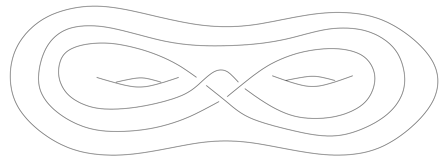
Figure 4. The 3-manifold $M_{2}$ as a knot complement in the handlebody of genus 2. Source: [5, Figure 3]

In [5, Section 2], Frigerio constructs an ideal triangulation of $M_{g}$. This construction is illustrated for the cases $g=2$ and $g=3$ in Figure 5. Let $P_{g}$ be the double cone with apices $ap_{1}$ and $ap_{2}$ and based on the regular ($2g+2$)-gon whose vertices are $p_{0}$, $p_{1}$, …, $p_{2g+1}$. Let $\mathring{P}_{g}$ be $P_{g}$ with its vertices removed. Let $Y_{g}$ be the topological space obtained by gluing the faces of $\mathring{P}_{g}$ according to the following rules:

• For any $i=0,2,...,2g$ , the face $[ap_{1},p_{i},p_{i+1}]$ is identified with the face $[p_{i+1},p_{i+2},v_{2}]$ (with $v_{1}$ identified with $p_{i+1}$, $p_{i}$ identified with $p_{i+2}$ and $p_{i+1}$ identified with $ap_{2}$),

• For any $i=1,3,...,2g+1$ , the face $[ap_{1},p_{i},p_{i+1}]$ is identified with the face $[p_{i+2},v_{2},p_{i+1}]$ (with $ap_{1}$ identified with $p_{i+2}$, $p_{i}$ identified with $ap_{2}$ and $p_{i+1}$ identified with $p_{i+1}$).

Proposition 4.2 (Proposition 2.1, [5]).

For any $g\geq 2$, $Y_{g}$ is homeomorphic to the interior of $M_{g}$.

We can then subdivide $P_{g}$ into $2g+2$ tetrahedra by adding the vertical edge between the two apices $ap_{1}$ and $ap_{2}$ (in red in Figure 5). Such tetrahedra give an ideal triangulation of $M_{g}$.

Figure 5. Representation of $Y_{2}$ (left) and $Y_{3}$ (right) with the red vertical edge between the two apices and identified edges and vertices have the same color.

4.2. Ordered triangulations and comb representation

We refer to [1, 11] for the following definitions. A triangulation is called ordered when it is endowed with an order on each quadruplet of vertices of each tetrahedron, such that the face gluings respect the vertex order. An equivalent property is that we can orient the edges of the triangulation in a compatible way with the face gluings and such that there are no cycles of length $3$.

Figure 6. An ordered tetrahedron $T$ (right) and its associated comb $C(T)$ (left).

A comb $C$ is a line together with four spikes pointing in the same direction. The spikes are numbered 0, 1, 2 and 3 going from left to right, with the spikes pointing upward. The comb representation of an ordered triangulation consists in associating a comb $C(T)$ to each tetrahedron $T$ of the triangulation, as in Figure 6; each spike numbered $i$ corresponds to a face $f^{i}$ opposed to a vertex $v_{i}$ for $i\in\{0,1,2,3\}$, and we join by a line the spike $i$ of $C(T)$ to the spike $j$ of $C(T^{\prime})$ if the $i$-th face of $T$ is glued to the $j$-th face of $T^{\prime}$.

The comb representation provides a compact way of representing an ordered triangulation, while containing all the information of this triangulation. Moreover, comb representations are convenient for studying certain quantum invariants of ordered triangulations (such as the Teichmüller TQFT [1]). In this sense, it is interesting to observe when a given triangulation admits an ordered structure. This is the case for Firgerio’s triangulations $\mathcal{T}_{g}$, as we now state:

Proposition 4.3.

The triangulations $\mathcal{T}_{g}$ of the manifolds $M_{g}$ admit an ordered structure.

The proof is quite standard, in that we exhibit a specific ordered structure (more details are in [7]). For brevity we will only refer to the examples of $g=2$ and $g=3$ represented in Figures 12 and 15. The associated comb representation for $g=2$ is drawn on Figure 7.

Figure 7. Comb representation of $\mathcal{T}_{2}$.

4.3. Hyperbolic structure

In [5, Section 2], Frigerio provides the unique angle structure on the tetrahedra of the ideal triangulation $\mathcal{T}_{g}$ that corresponds to the unique complete hyperbolic structure on the manifold $M_{g}$. Setting $\alpha_{g}=\frac{\pi}{2g+2}$ , $\beta_{g}=2\alpha_{g}$, $\gamma_{g}=\arccos((2\cos\alpha_{g})^{-1})$ and $\delta_{g}=\pi-2\gamma_{g}$, the complete angle structure on $\mathcal{T}_{g}$ follows the pattern of Figure 8: half of the $2g+2$ tetrahedra are as the one on the left, and the other half are as the one on the right.

Figure 8. Frigerio’s angle structure on $\mathcal{T}_{g}$

Both tetrahedra of Figure 8 have the same volume, and the volume of $M_{g}$ is exactly $2g+2$ times higher. Values of these volumes are computed with SageMath (see Section 5.1.2) and listed in Figure 9.

4.4. Admissible colorings

In this section we study the set of admissible colorings for the triangulations $\mathcal{T}_{g}$. The following three lemmas follow from standard arguments, are not restricted to the manifolds $M_{g}$, and will be used in the proof of Theorem 4.8. See [7] for details.

Lemma 4.4.

Let $i,k\in I_{r}$. Then $(i,i,k)$ is admissible if and only if $k\in\mathbb{N}$ and $\frac{k}{2}\leq i\leq\frac{r-2-k}{2}$.

Lemma 4.5.

Let $i,j,k,l,m\in I_{r}$ such that $(i,j,k)$ and $(k,l,m)$ are admissible, then $i+j+l+m\in\mathbb{N}$.

Lemma 4.6.

Let $i,j,k\in I_{r}$ such that $k\in\mathbb{N}$. Then the following conditions are equivalent:

1. $i+j+k\in\mathbb{N}$,

2. $i+j\in\mathbb{N}$,

3. either $i,j\in\mathbb{N}$ or $i,j\in\frac{\mathbb{N}_{odd}}{2}$.

Remark 4.7.

Lemma 4.6 can be applied to condition (ii) of Definition 3.3 when $i$, $j$ or $k$ is in $\mathbb{N}$.

Let $g\in\mathbb{N}_{\geq 2}$. For a general coloring $c$ at level $r$ of $(M_{g},\mathcal{T}_{g})$, we need the following triples of elements of $I_{r}$ to be admissible:

$(a,b,b)$,	$(a,c_{g},c_{0})$,	$(b,c_{g},c_{g})$,	$(b,c_{g},c_{0})$,
and for all $i\in\left\{0,1,2,...,g-1\right\}$,	$(a,c_{i},c_{i+1})$,	$(b,c_{i},c_{i})$,	$(b,c_{i},c_{i+1})$.

These admissibility conditions can be rewritten like in the next theorem.

Theorem 4.8.

Let $a$, $b$, $c_{0}$, $c_{1}$, $c_{2}$, …, $c_{g}\in I_{r}$.

The conditions $(A)$, $(B)$, $(C)$, $(D)$, $(E)$, $(F)$ and $(G)$ defined below are simultaneously satisfied if and only if the conditions $(1)$, $(2)$, $(3)$, $(4)$, $(5)$ and $(6)$ defined below are simultaneously satisfied.

The conditions $(A)$, $(B)$, $(C)$, $(D)$, $(E)$, $(F)$ and $(G)$ are written:

1. $(a,b,b)$ is admissible,

2. $(a,c_{g},c_{0})$ is admissible,

3. $(b,c_{g},c_{g})$ is admissible,

4. $(b,c_{g},c_{0})$ is admissible,

5. $\forall i\in\left\{0,1,2,...,g-1\right\}$, $(a,c_{i},c_{i+1})$ is admissible,

6. $\forall i\in\left\{0,1,2,...,g-1\right\}$, $(b,c_{i},c_{i})$ is admissible,

7. $\forall i\in\left\{0,1,2,...,g-1\right\}$, $(b,c_{i},c_{i+1})$ is admissible,

The conditions $(1)$, $(2)$, $(3)$, $(4)$, $(5)$ and $(6)$ are written:

1. $a\in\mathbb{N}$,

2. $b\in\mathbb{N}$,

3. either $\forall i\in\left\{0,1,2...,g\right\}$, $c_{i}\in\mathbb{N}$ or $\forall i\in\left\{0,1,2,...,g\right\}$, $c_{i}\in\frac{\mathbb{N}_{odd}}{2}$,

4. $\frac{a}{2}\leq b\leq\frac{r-2-a}{2}$,

5. 1. $\forall i\in\left\{0,1,2...,g-1\right\}$, $\frac{b}{2}\leq c_{i+1}\leq\frac{r-2-b}{2}$,

   2. $\forall i\in\left\{0,1,2...,g-1\right\}$, $a-c_{i}\leq c_{i+1}\leq r-2-a-c_{i}$,

   3. $\forall i\in\left\{0,1,2...,g-1\right\}$, $c_{i}-a\leq c_{i+1}\leq a+c_{i}$,

   4. $\forall i\in\left\{0,1,2...,g-1\right\}$, $c_{i}-b\leq c_{i+1}\leq b+c_{i}$,

6. 1. $\frac{b}{2}\leq c_{0}\leq\frac{r-2-b}{2}$,

   2. $a-c_{g}\leq c_{0}\leq r-2-a-c_{g}$,

   3. $c_{g}-a\leq c_{0}\leq a+c_{g}$,

   4. $c_{g}-b\leq c_{0}\leq b+c_{g}$.

Proof.

Let $a$, $b$, $c_{0}$, $c_{1}$, $c_{2}$, …, $c_{g}\in I_{r}$.

Step 1 : $(\ref{conditionA})\iff(\ref{condition1})\wedge(\ref{condition4})$;

This step follows immediately from Lemma 4.4.

Step 2 : $(\ref{conditionA})\wedge(\ref{conditionE})\iff(\ref{condition1})\wedge(\ref{condition3})\wedge(\ref{condition4})\wedge(\ref{condition5b})\wedge(\ref{condition5c})$;

By Definition 3.3, Condition $(\ref{conditionE})$ is equivalent to the following conditions :

1. 1. $\forall i\in\left\{0,1,2...,g-1\right\}$, $c_{i}+c_{i+1}\geq a$,

   2. $\forall i\in\left\{0,1,2...,g-1\right\}$, $c_{i}+a\geq c_{i+1}$,

   3. $\forall i\in\left\{0,1,2...,g-1\right\}$, $a+c_{i+1}\geq c_{i}$,

2. $\forall i\in\left\{0,1,2...,g-1\right\}$, $c_{i}+c_{i+1}+a\in\mathbb{N}$,

3. $\forall i\in\left\{0,1,2...,g-1\right\}$, $c_{i}+c_{i+1}+a\leq r\scalebox{1.8}[1.0]{-}2$.

To prove Step 2, we first remark that:

$$(E\ref{ia})\wedge(E\ref{iii})\iff(\ref{condition5b}),$$

$$(E\ref{ib})\wedge(E\ref{ic})\iff(\ref{condition5c}).$$

It remains to prove that :

$$(\ref{conditionA})\wedge(E\ref{ii})\iff(\ref{condition1})\wedge(\ref{condition3})\wedge(\ref{condition4}).$$

It follows from Step 1 that :

$$(\ref{conditionA})\wedge(E\ref{ii})\iff(\ref{condition1})\wedge(\ref{condition4})\wedge(E\ref{ii}).$$

From Lemma 4.6, it follows that

$$(\ref{condition1})\wedge(\ref{condition4})\wedge(E\ref{ii})\iff(\ref{condition1})\wedge(\ref{condition4})\wedge\left(\forall i\in\left\{0,1,2...,g-1\right\},\left(c_{i},c_{i+1}\in\mathbb{N}\right)\lor\left(c_{i},c_{i+1}\in\frac{\mathbb{N}_{odd}}{2}\right)\right).$$

Finally, it follows by a quick induction that:

$$(\ref{condition1})\wedge(\ref{condition4})\wedge\left(\forall i\in\left\{0,1,2...,g-1\right\},\left(c_{i},c_{i+1}\in\mathbb{N}\right)\lor\left(c_{i},c_{i+1}\in\frac{\mathbb{N}_{odd}}{2}\right)\right)\iff(\ref{condition1})\wedge(\ref{condition4})\wedge(\ref{condition3}).$$

Step 3 : $(\ref{conditionA})\wedge(\ref{conditionB})\wedge(\ref{conditionE})\iff(\ref{condition1})\wedge(\ref{condition3})\wedge(\ref{condition4})\wedge(\ref{condition5b})\wedge(\ref{condition5c})\wedge(\ref{condition6b})\wedge(\ref{condition6c})$;

From Step 2, it follows that:

$$(\ref{conditionA})\wedge(\ref{conditionE})\iff(\ref{condition1})\wedge(\ref{condition3})\wedge(\ref{condition4})\wedge(\ref{condition5b})\wedge(\ref{condition5c}).$$

By Definition 3.3, Condition $(\ref{conditionB})$ is equivalent to the following conditions :

1. 1. $c_{g}+c_{0}\geq a$,

   2. $c_{g}+a\geq c_{0}$,

   3. $a+c_{0}\geq c_{g}$,

2. $c_{g}+c_{0}+a\in\mathbb{N}$,

3. $c_{g}+c_{0}+a\leq r\scalebox{1.8}[1.0]{-}2$.

To prove Step 3, we first remark that:

$$(B\ref{iaB})\wedge(B\ref{iiiB})\iff(\ref{condition6b}),$$

$$(B\ref{ibB})\wedge(B\ref{icB})\iff(\ref{condition6c}).$$

Finally, let us prove the following implication which will imply Step 3:

$$(\ref{conditionA})\wedge(\ref{conditionE})\implies(B\ref{iiB}).$$

From Step 2, it follows that

$$(\ref{conditionA})\wedge(\ref{conditionE})\implies(\ref{condition1})\wedge(\ref{condition3}).$$

Furthermore, using Lemma 4.6, we have that:

$$(\ref{condition1})\wedge(\ref{condition3})\implies(B\ref{iiB}).$$

Step 4 : $(\ref{conditionC})\wedge(\ref{conditionF})\iff(\ref{condition2})\wedge(\ref{condition5a})\wedge(\ref{condition6a})$;

This step follows immediately from Lemma 4.4.

Step 5 : $(\ref{conditionA})\wedge(\ref{conditionB})\wedge(\ref{conditionC})\wedge(\ref{conditionE})\wedge(\ref{conditionF})\wedge(\ref{conditionG})\iff$
$(\ref{condition1})\wedge(\ref{condition2})\wedge(\ref{condition3})\wedge(\ref{condition4})\wedge(\ref{condition5a})\wedge(\ref{condition5b})\wedge(\ref{condition5c})\wedge(\ref{condition5d})\wedge(\ref{condition6a})\wedge(\ref{condition6b})\wedge(\ref{condition6c})$;

From Step 3, it follows that:

$$(\ref{conditionA})\wedge(\ref{conditionB})\wedge(\ref{conditionE})\iff(\ref{condition1})\wedge(\ref{condition3})\wedge(\ref{condition4})\wedge(\ref{condition5b})\wedge(\ref{condition5c})\wedge(\ref{condition6b})\wedge(\ref{condition6c}).$$

From Step 4, it follows that:

$$(\ref{conditionC})\wedge(\ref{conditionF})\iff(\ref{condition2})\wedge(\ref{condition5a})\wedge(\ref{condition6a}).$$

By Definition 3.3, Condition $(\ref{conditionG})$ is equivalent to the following conditions :

1. 1. $\forall i\in\left\{0,1,2...,g-1\right\}$, $c_{i}+c_{i+1}\geq b$,

   2. $\forall i\in\left\{0,1,2...,g-1\right\}$, $c_{i}+b\geq c_{i+1}$,

   3. $\forall i\in\left\{0,1,2...,g-1\right\}$, $b+c_{i+1}\geq c_{i}$,

2. $\forall i\in\left\{0,1,2...,g-1\right\}$, $c_{i}+c_{i+1}+b\in\mathbb{N}$,

3. $\forall i\in\left\{0,1,2...,g-1\right\}$, $c_{i}+c_{i+1}+b\leq r\scalebox{1.8}[1.0]{-}2$.

Following what precedes, in order to prove Step 5, we only need to prove that:

1. $(\ref{conditionC})\wedge(\ref{conditionF})\implies(G\ref{iab})\wedge(G\ref{iiib})$,

2. $(G\ref{ibb})\wedge(G\ref{icb})\iff(\ref{condition5d})$,

3. $(\ref{conditionA})\wedge(\ref{conditionE})\implies(G\ref{iib})$.

Let us prove Step 5.1. From Step 4, it follows that

$$(\ref{conditionC})\wedge(\ref{conditionF})\implies(\ref{condition5a})\wedge(\ref{condition6a}).$$

Furthermore, we have by adding inequalities that :

$$(\ref{condition5a})\wedge(\ref{condition6a})\implies(G\ref{iab})\wedge(G\ref{iiib}).$$

Step 5.2 follows immediately from the definitions.

Finally, let us prove Step 5.3. From Step 2, it follows that

$$(\ref{conditionA})\wedge(\ref{conditionE})\implies(\ref{condition1})\wedge(\ref{condition3}).$$

Furthermore, using Lemma 4.6, we have that:

$$(\ref{condition1})\wedge(\ref{condition3})\implies(G\ref{iib}).$$

This concludes the proof of Step 5.

Step 6 : $(\ref{conditionA})\wedge(\ref{conditionB})\wedge(\ref{conditionC})\wedge(\ref{conditionD})\wedge(\ref{conditionE})\wedge(\ref{conditionF})\wedge(\ref{conditionG})\iff$
$(\ref{condition1})\wedge(\ref{condition2})\wedge(\ref{condition3})\wedge(\ref{condition4})\wedge(\ref{condition5a})\wedge(\ref{condition5b})\wedge(\ref{condition5c})\wedge(\ref{condition5d})\wedge(\ref{condition6a})\wedge(\ref{condition6b})\wedge(\ref{condition6c})\wedge(\ref{condition6d})$;

We prove Step 6 almost exactly as we proved Step 5. The only difference being the $(G)$ conditions become $(D)$ conditions and $(5d)$ becomes $(6d)$.

This concludes the proof of the theorem. ∎

As we will see, Theorem 4.8 can be used to simplify the formula and computation of the Turaev–Viro invariants for the manifolds $M_{g}$, and to write a code for computing these invariants numerically (see Section 5.2).

5. Annotated code

The following codes have been written with SageMath, a free open-source mathematics software system using Python 3. In this section, let us fix a pair $(r,s)\in\mathbb{N}^{2}$ such that $r\geq 3$ and $s\geq 1$. Let $g\in\mathbb{N}_{\geqslant 2}$. Let us recall the following notation:

Notation 5.1.

Let $\frac{\mathbb{N}}{2}=\{0,\frac{1}{2},1,...\}$ denote the set of non-negative half integers. Let $\frac{\mathbb{N}_{odd}}{2}=\{\frac{1}{2},\frac{3}{2},...\}$ denote the set of non-negative half-odd-integers. Let $I_{r}$ denote the subset $\left\{0,\frac{1}{2},1,...,\frac{r-2}{2}\right\}$ of $\frac{\mathbb{N}}{2}$.

5.1. Computing the hyperbolic volume of $M_{g}$

In this section, we construct a function which computes the volume of a tetrahedron from its dihedral angles, via Ushijima’s volume formula (see Proposition 3.1). We then apply this function to the manifolds $M_{g}$ with triangulations $\mathcal{T}_{g}$.

5.1.1. The volume formula for hyperbolic tetrahedra

We follow the steps and notation of Section 3.2. We first import the NumPy package which is an easy to use, open source package in Python. This package contains the function pi giving an approximate value of $\pi$ that we will use later on. Functions imported from this package will be written in the code with the prefix np., which means we access the function inside the package NumPy. The function Gramdet(A,B,C,D,E,F) computes the determinant of the Gram matrix associated to $A,B,C,D,E,F\in\left[0,\pi\right]$.

⬇

1import numpy as np

2

3def Gramdet(A,B,C,D,E,F):

4G = matrix([ [1,-cos(A),-cos(B),-cos(F)],

5[-cos(A),1,-cos(C),-cos(E)],

6[-cos(B),-cos(C),1,-cos(D)],

7[-cos(F),-cos(E),-cos(D),1]])

8res = G.determinant()

9return res

Listing 1: The determinant of the Gram matrix of $T$

The U(z,A,B,C,D,E,F) function computes $U(z,T)$ for a given complex number $z$ and the dihedral angles $A,B,C,D,E$ and $F$ of a given generalized tetrahedron $T$. We use the dilog(z) function for $z$ a complex number to compute $\mathrm{Li_{2}}(z)$.

⬇

1def U(z,A,B,C,D,E,F):

2a = exp(I*A)

3b = exp(I*B)

4c = exp(I*C)

5d = exp(I*D)

6e = exp(I*E)

7f = exp(I*F)

8

9z1 = a*b*d*e*z

10z2 = a*c*d*f*z

11z3 = b*c*e*f*z

12z4 = -a*b*c*z

13z5 = -a*e*f*z

14z6 = -b*d*f*z

15z7 = -c*d*e*z

16

17res = 1/2*(dilog(z)+dilog(z1)+dilog(z2)+dilog(z3)-dilog(z4)-dilog(z5)-dilog(z6)-dilog(z7))

18return res

Listing 2: The complex valued fonction $U(z,T)$

Finally, the TetVolum(A,B,C,D,E,F) function uses the formula of Proposition 3.1 to compute the hyperbolic volume of a tetrahedron given its dihedral angles $A$, $B$, $C$, $D$, $E$ and $F$.

⬇

1def TetVolum(A,B,C,D,E,F):

2a = exp(I*A)

3b = exp(I*B)

4c = exp(I*C)

5d = exp(I*D)

6e = exp(I*E)

7f = exp(I*F)

8

9det = Gramdet(A,B,C,D,E,F)

10

11zminus = -2*((sin(A)*sin(D)+sin(B)*sin(E)+sin(C)*sin(F)-sqrt(det))/(a*d+b*e+c*f+a*b*f+a*c*e+b*c*d+d*e*f+a*b*c*d*e*f))

12

13zplus = -2*((sin(A)*sin(D)+sin(B)*sin(E)+sin(C)*sin(F)+sqrt(det))/(a*d+b*e+c*f+a*b*f+a*c*e+b*c*d+d*e*f+a*b*c*d*e*f))

14

15res = imag((U(zminus,A,B,C,D,E,F)-U(zplus,A,B,C,D,E,F))/2)

16return res

Listing 3: The hyperbolic volume of $T$

5.1.2. Applying the volume formula on tetrahedra of $\mathcal{T}_{g}$

Following Frigerio’s computation of the complete angle structure detailed in Section 4.3, we define the function HyperbolicVolume(g) to compute the hyperbolic volume of $M_{g}$ given $g\in\{2,3,4,...\}$. Thanks to the symmetries in the complete angle structure, this function computes the hyperbolic volume of one tetrahedron and multiplies it by $2g+2$ (the number of tetrahedra in the triangulation). We display several values for this function for some values of $g$ in Figure 9.

⬇

1def HyperbolicVolume(g):

2Alphag=np.pi/(2*g+2)

3Betag=2*Alphag

4Gammag=arccos(1/(2*cos(Alphag)))

5Deltag=np.pi - 2*Gammag

6

7res=(2*g+2)*TetVolum(Gammag,Deltag,Gammag,Alphag,Betag,Alphag)

8return res

Listing 4: The hyperbolic volume of $M_{g}$ for a given $g$

$g$	$\mathrm{Vol}(T_{g})$	$\mathrm{Vol}(M_{g})$
2	2.007682006682397	12.046092040094381
3	2.2547631818606026	18.03810545488482
4	2.3603494908554774	23.603494908554772
5	2.415787949187158	28.989455390245897
6	2.448617485457304	34.28064479640226
7	2.469695490891516	39.51512785426426
8	2.484045062029212	44.71281111652581
9	2.494259571737797	49.88519143475594
10	2.5017908556003303	55.039398823207264
100	2.5369350366401	512.4608774013002
1000	2.5373497508910896	5079.774201283962

Figure 9. The hyperbolic volumes of $M_{g}$ and one tetrahedron $T_{g}$ of $\mathcal{T}_{g}$ for various values of $g$.

5.2. Computing the Turaev–Viro invariants $TV_{r,s}(M_{g},\mathcal{T}_{g})$

In this section, we will construct several functions in order to compute the Turaev–Viro invariants $TV_{r,s}(M_{2},\mathcal{T}_{2})$ and $TV_{r,s}(M_{3},\mathcal{T}_{3})$ given $(r,s)\in\mathbb{N}^{2}$ such that $r\geq 3$ and $s\geq 1$. These functions can easily be extended to compute the other Turaev–Viro invariants $TV_{r,s}(M_{g},\mathcal{T}_{g})$ for $g\geq 4$ (which we will do for $4\leqslant g\leqslant 7$).

We first import the NumPy package as in Section 5.1.1. We also import the cmath package which gives us mathematical functions for complex numbers, such as square roots for negative numbers. Functions imported from cmath will be written with the prefix cm..

⬇

1import numpy as np

2import cmath as cm

Listing 5: Importing NumPy and cmath

The function quantum_number(r,s,n) returns the quantum number $[n]$ given $r$, $s$ and $n\in\mathbb{N}$.

⬇

1def quantum_number(r,s,n):

2res=sin(s*n*(np.pi)/r)/sin(s*(np.pi)/r)

3return res

Listing 6: Quantum number

The function quantum_factorial(r,s,n) returns the factorial of a quantum number $[n]!$ given $r$, $s$ and $n\in\mathbb{N}$.

⬇

1def quantum_factorial(r,s,n):

2if n == 0:

3return 1

4return prod([quantum_number(r,s,i) for i in range(1, n+1)])

Listing 7: Quantum factorial

The function q_big_delta_coeff(i,j,k,r,s) returns the coefficients $\Delta(i,j,k)$ given $r$, $s$ and $(i,j,k)$ an admissible triple of elements of $I_{r}$. Admissibility conditions ensure that $i+j-k$, $i+k-j$, $j+k-i$ and $i+j+k+1$ are in $\mathbb{N}$ but since the values of $i$, $j$ and $k$ can be half integers, the values $i+k-j$, $j+k-i$ and $i+j+k+1$ are stored as rational type variable. To ensure that the function quantum_factorial() works, we have to change their type from rational to integers using the $int()$ function. Since quantum_number() and thus quantum_factorial() can return negative values, the term we take the square root of might thus be negative. Hence we need to use the function cm.sqrt(), i.e the complex square root from the cmath package.

⬇

1def q_big_delta_coeff(i,j,k,r,s):

2argsqrt = (quantum_factorial(r,s,int(i + j - k)) * quantum_factorial(r,s,int(i + k - j)) * quantum_factorial(r,s,int(j + k - i))) / quantum_factorial(r,s,int(i + j + k + 1))

3

4res = cm.sqrt(argsqrt)

5return res

Listing 8: $\Delta$ coefficients

The function q_symbol(i, j, k, l, m, n, r, s) returns the quantum $6j$-symbol $\begin{vmatrix}i&j&k\\ l&m&n\end{vmatrix}$ given $r$, $s$ and $(i,j,k,l,m,n)$ a sextuple of elements of $I_{r}$ such that $(i,j,k)$, $(j,l,n)$, $(i,m,n)$ and $(k,l,m)$ are admissible.

⬇

1def q_symbol(i, j, k, l, m, n, r, s):

2prefac = q_big_delta_coeff(i, j, k, r, s) * q_big_delta_coeff(j, l, n, r, s) * q_big_delta_coeff(i, m, n, r, s) * q_big_delta_coeff(k, l, m, r, s)

3

4zmin = max(i + j + k, j + l + n, i + m + n, k + l + m)

5zmax = min(i + j + l + m, i + k + l + n, j + k + m + n)

6

7sumres = 0

8for z in range(int(zmin), int(zmax) + 1):

9den = quantum_factorial(r,s,int(z - (i + j + k))) * quantum_factorial(r,s,int(z - (j + l + n))) * quantum_factorial(r,s,int(z - (i + m + n))) * quantum_factorial(r,s,int(z - (k + l + m))) * quantum_factorial(r,s,int(i + j + l + m - z)) * quantum_factorial(r,s,int(i + k + l + n - z)) * quantum_factorial(r,s,int(j + k + m + n - z))

10

11sumres = sumres + (((-1) ** z) * quantum_factorial(r,s,int(z + 1))) / den

12

13res = prefac * sumres * sqrt(-1)**(int(2*(i+j+k+l+m+n)))

14return res

Listing 9: Quantum $6j$-symbols

The function edge(a,r,s) yields the term $w_{a}:=(\scalebox{1.8}[1.0]{-}1)^{2a}[2a+1]$ for $r$, $s$ and $a\in I_{r}$.

⬇

1def edge(a,r,s) :

2res = ((-1)**(2*a))*quantum_number(r,s,int(2*a+1))

3return res

Listing 10: Edge term

The function term(a,b,c,g,r,s) computes one term of the sum in the Definition 3.7 applied to $(M_{g},\mathcal{T}_{g})$ given $r$, $s$ as before, $g\in\{2,3,4,...\}$, $a\in I_{r}$, $b\in I_{r}$ and $c=(c_{0},c_{1},c_{2},...,c_{g})\in I_{r}^{g+1}$ satisfying the conditions in Theorem 4.8. This one term is equal to the product of $w_{a}w_{b}w_{c_{0}}\ldots w_{c_{g}}$ with

$$\scriptsize\begin{vmatrix}a&b&b\\ c_{0}&c_{0}&c_{g}\end{vmatrix}\begin{vmatrix}a&b&b\\ c_{0}&c_{0}&c_{1}\end{vmatrix}\ldots\begin{vmatrix}a&b&b\\ c_{i}&c_{i}&c_{i-1}\end{vmatrix}\begin{vmatrix}a&b&b\\ c_{i}&c_{i}&c_{i+1}\end{vmatrix}\ldots\begin{vmatrix}a&b&b\\ c_{g}&c_{g}&c_{g-1}\end{vmatrix}\begin{vmatrix}a&b&b\\ c_{g}&c_{g}&c_{0}\end{vmatrix}.$$

⬇

1def term(a,b,c,g,r,s):

2res=edge(a, r, s)*edge(b, r, s)

3

4for i in range(g+1):

5if i==0:

6res = res * edge(c[i], r, s) * q_symbol(a, b, b, c[i], c[i], c[g], r, s) * q_symbol(a, b, b, c[i], c[i], c[i+1], r, s)

7elif i==g:

8res = res * edge(c[i], r, s) * q_symbol(a, b, b, c[i], c[i], c[i-1], r, s) * q_symbol(a, b, b, c[i], c[i], c[0], r, s)

9else:

10res = res * edge(c[i], r, s) * q_symbol(a, b, b, c[i], c[i], c[i-1], r, s) * q_symbol(a, b, b, c[i], c[i], c[i+1], r, s)

11

12return res

Listing 11: One term of the sum in $TV_{r,s}(M_{g},\mathcal{T}_{g})$ for a given admissible coloring

The function turaevvirog2(r,s) computes $TV_{r,s}(M_{2},\mathcal{T}_{2})$, while the function turaevvirog3(r,s) computes $TV_{r,s}(M_{3},\mathcal{T}_{3})$ given $r$ and $s$. These two functions consists in listing all the admissible colorings in the sense of Theorem 4.8 and computing the associated term contributing to the sum in $TV_{r,s}(M_{g},\mathcal{T}_{g})$ via the term() function for $g\in\{2,3\}$.

We now detail the reasoning behind the following code. Let $a,b,c_{0},...,c_{g}\in I_{r}$.

The $a$ loop: For the coloring to be admissible, $a$ has to satisfy:

• $a\in\mathbb{N}$.

The first loop is over the label $a$ which covers all integers from $0$ to $\frac{r-2}{2}$. We will refer to it as the $a$ loop. The floor() function ensures that the loop ends at $\left\lfloor{\frac{r-2}{2}}\right\rfloor$.

The $b$ loop: For $a$ fixed and an admissible coloring, $b$ has to satisfy:

• $b\in\mathbb{N}$,

• $\frac{a}{2}\leq b\leq\frac{r-2-a}{2}$.

We thus create, inside the $a$ loop, a second loop over the label $b$ (called the $b$ loop), which covers all integers from $\frac{a}{2}$ to $\frac{r-2-a}{2}$. The floor() and ceil() functions ensure that the loop ends at $\left\lfloor{\frac{r-2-a}{2}}\right\rfloor$ and starts at $\left\lceil{\frac{a}{2}}\right\rceil$.

The two kinds of nested loops inside the $b$ loop: For an admissible coloring, the labels $c_{i}$ (for $i\in\{0,1,2,...,g\}$) have to satisfy:

• either ($\forall i\in\{0,1,2,...,g\}$, $c_{i}\in\mathbb{N}$) or ($\forall i\in\{0,1,2,...,g\}$, $c_{i}\in\frac{\mathbb{N}_{odd}}{2}$).

We denote those two categories as integer states and half-integer states. Thus, we create two different loops inside the $b$ loop (one for each).

The first family of nested loops, for integer states: Let us assume ($\forall i\in\{0,\ldots,g\}$, $c_{i}\in\mathbb{N}$). For a fixed $b$ and an admissible coloring, the label $c_{0}$ has to satisfy:

• $\frac{b}{2}\leq c_{0}\leq\frac{r-2-b}{2}$.

We thus create, inside the $b$ loop, a loop over the label $c_{0}$, the $c_{0}$ loop, which covers all integers from $\left\lceil{\frac{b}{2}}\right\rceil$ to $\left\lfloor{\frac{r-2-b}{2}}\right\rfloor$. This $c_{0}$ loop will contain a new $c_{1}$ loop, which will in turn contain a $c_{2}$ loop, and so on until a final $c_{g}$ loop. Let us now detail how this induction works. For $i\in\{0,...,g-1\}$, for fixed $a$, $b$, $c_{i}$ and an admissible coloring, the label $c_{i+1}$ has to satisfy the following conditions:

• $\frac{b}{2}\leq c_{i+1}\leq\frac{r-2-b}{2}$,

• $a-c_{i}\leq c_{i+1}\leq r-2-a-c_{i}$,

• $c_{i}-\min(a,b)\leq c_{i+1}\leq c_{i}+\min(a,b)$.

For all $i\in\{0,...,g-1\}$, we create in the loop $c_{i}$ two variables $m_{i+1}$ and $M_{i+1}$: $m_{i+1}$ is the maximum of the three lower bounds on $c_{i+1}$ and $M_{i+1}$ is the minimum of the three upper bounds on $c_{i+1}$. We thus create, inside the $c_{i}$ loop, a loop over the label $c_{i+1}$ (called the $c_{i+1}$ loop), which ranges to all integers from $\left\lceil{m_{i+1}}\right\rceil$ to $\left\lfloor{M_{i+1}}\right\rfloor$. Finally, for fixed $a$, $b$, $c_{0},\ldots,c_{g}$, for the coloring to be admissible, the following conditions also need to be satisfied:

• $a-c_{g}\leq c_{0}\leq r-2-a-c_{g}$,

• $c_{g}-\min(a,b)\leq c_{0}\leq c_{g}+\min(a,b)$.

Hence we add an if loop that checks those two conditions. If they are satisfied, we then compute the term associated to the coloring $(a,b,c_{0},c_{1},...,c_{g})$ via term().

The second family of nested loops, for half-integer states: Once we have covered all the integer states, we create inside the $b$ loop, a second loop over the label $c_{0}$, which covers all half-integers from $\left\lfloor{\frac{b}{2}}\right\rfloor+\frac{1}{2}$ to $\left\lceil{\frac{r-2-b}{2}}\right\rceil-\frac{1}{2}$. The function np.arange() allows us to start and end loops at non-integer values and specify the step of the loop to be 1. The rest of this new $c_{0}$ loop is constructed in the same way as for the $c_{0}$ loop for integer states, but the nested loops are over half-integers instead of integers.

Conclusion: As proved in Theorem 4.8, these loops go over all admissible states, thus we obtain a numerical value of the exact formula $TV_{r,s}(M_{g},\mathcal{T}_{g})$ for $g\in\{2,3\}$. In the same way, one can construct a function which computes $TV_{r,s}(M_{g},\mathcal{T}_{g})$ for $g\geq 4$ (one would simply need to add more nested loops in the two families). In the current project, we did exactly this: we defined the functions turaevvirog4(r,s), turaevvirog5(r,s), turaevvirog6(r,s) and turaevvirog7(r,s), but for the sake of brevity we do not write their codes here (their codes can be easily guessed from the detailed examples of turaevvirog2(r,s) and turaevvirog3(r,s)).

⬇

1def turaevvirog2(r,s):

2res= 0

3for a in range(floor((r-2)/2)+1):

4for b in range(ceil(a/2),floor((r-2-a)/2)+1):

5m=min(a,b)

6for c0 in range(ceil(b/2),floor((r-2-b)/2)+1):

7m1=max(c0-m,a-c0,b/2)

8M1=min(c0+m,r-2-a-c0,(r-2-b)/2)

9for c1 in range(ceil(m1),floor(M1)+1):

10m2=max(c1-m,a-c1,b/2)

11M2=min(c1+m,r-2-a-c1,(r-2-b)/2)

12for c2 in range(ceil(m2),floor(M2)+1):

13if (-m<=c2-c0<=m) and (a<=c2+c0<=r-2-a):

14c=[c0,c1,c2]

15res=res+term(a,b,c,2,r,s)

16

17for c0 in np.arange(floor(b/2)+1/2,ceil((r-2-b)/2),1):

18m1=max(c0-m,a-c0,b/2)

19M1=min(c0+m,r-2-a-c0,(r-2-b)/2)

20for c1 in np.arange(floor(m1)+1/2,ceil(M1),1):

21m2=max(c1-m,a-c1,b/2)

22M2=min(c1+m,r-2-a-c1,(r-2-b)/2)

23for c2 in np.arange(floor(m2)+1/2,ceil(M2),1):

24if (-m<=c2-c0<=m) and (a<=c2+c0<=r-2-a):

25c=[c0,c1,c2]

26res=res+term(a,b,c,2,r,s)

27return res

Listing 12: $TV_{r,s}(M_{2},\mathcal{T}_{2})$

⬇

1def turaevvirog3(r,s):

2res= 0

3for a in range(floor((r-2)/2)+1):

4for b in np.arange(ceil(a/2),floor((r-2-a)/2)+1,1):

5m=min(a,b)

6for c0 in np.arange(ceil(b/2),floor((r-2-b)/2)+1,1):

7m1=max(c0-m,a-c0,b/2)

8M1=min(c0+m,r-2-a-c0,(r-2-b)/2)

9for c1 in np.arange(ceil(m1),floor(M1)+1,1):

10m2=max(c1-m,a-c1,b/2)

11M2=min(c1+m,r-2-a-c1,(r-2-b)/2)

12for c2 in np.arange(ceil(m2),floor(M2)+1,1):

13m3=max(c2-m,a-c2,b/2)

14M3=min(c2+m,r-2-a-c2,(r-2-b)/2)

15for c3 in np.arange(ceil(m3),floor(M3)+1,1):

16if (-m<=c3-c0<=m) and (a<=c3+c0<=r-2-a):

17c=[c0,c1,c2,c3]

18res=res+term(a,b,c,3,r,s)

19

20for c0 in np.arange(floor(b/2)+1/2,ceil((r-2-b)/2),1):

21m1=max(c0-m,a-c0,b/2)

22M1=min(c0+m,r-2-a-c0,(r-2-b)/2)

23for c1 in np.arange(floor(m1)+1/2,ceil(M1),1):

24m2=max(c1-m,a-c1,b/2)

25M2=min(c1+m,r-2-a-c1,(r-2-b)/2)

26for c2 in np.arange(floor(m2)+1/2,ceil(M2),1):

27m3=max(c2-m,a-c2,b/2)

28M3=min(c2+m,r-2-a-c2,(r-2-b)/2)

29for c3 in np.arange(floor(m3)+1/2,ceil(M3),1):

30if (-m<=c3-c0<=m) and (a<=c3+c0<=r-2-a):

31c=[c0,c1,c2,c3]

32res=res+term(a,b,c,3,r,s)

33return res

Listing 13: $TV_{r,s}(M_{3},\mathcal{T}_{3})$

5.3. Asymptotic behavior of $QV_{r,2}(M_{2})$ and $QV_{r,2}(M_{3})$

The function quantumvirog2(r,s) computes $QV_{r,s}(M_{2})=\frac{s\pi}{r-2}\log\left(TV_{r,s}(M_{2},\mathcal{T}_{2})\right)$ given $(r,s)\in\mathbb{N}^{2}$ such that $r\geq 3$ and $s\geq 1$.

⬇

1def quantumvirog2(r,s):

2res=(s*(np.pi)/(r-2))*log(turaevvirog2(r,s))

3return res

Listing 14: $QV_{r,s}(M_{2},\mathcal{T}_{2})$

The function quantumvirog3(r,s) computes $QV_{r,s}(M_{3})=\frac{s\pi}{r-2}\log\left(TV_{r,s}(M_{3},\mathcal{T}_{3})\right)$ $(r,s)\in\mathbb{N}^{2}$ such that $r\geq 3$ and $s\geq 1$.

⬇

1def quantumvirog3(r,s):

2res=(s*(np.pi)/(r-2))*log(turaevvirog3(r,s))

3return res

Listing 15: $QV_{r,s}(M_{3},\mathcal{T}_{3})$

Similarly, the definitions of quantumvirog4(r,s), quantumvirog5(r,s), quantumvirog6(r,s) and quantumvirog7(r,s) follow immediately.

Let us recall that we aim for a numerical test of Conjecture 1.1. Thus, we set $s=2$ in order to numerically compute $QV_{r,2}(M_{2})$ and $QV_{r,2}(M_{3})$.

Note that, for some $r$ it happens that $TV_{r,2}(M_{2},\mathcal{T}_{2})$ is negative. Since we require the argument of the complex logarithm function to be in $[0,2\pi[$, the imaginary part of $QV_{r,2}(M_{2})$ is either 0 when $TV_{r,2}(M_{2},\mathcal{T}_{2})$ is positive or $\frac{2\pi^{2}}{r}$ when $TV_{r,2}(M_{2},\mathcal{T}_{2})$ is negative, which converges to $0$ as $r\to\infty$. Therefore to test the convergence of $QV_{r,2}(M_{2})$ we can forget about imaginary parts and consider only the real parts.

We compute the function quantumvirog2(r,s) for $s=2$ and increasing values of $r$, and we obtain the table of values of $\mathcal{R}\left(QV_{r,2}(M_{2})\right)$ shown in Figure 10. We use the numerical approximation .n() with the best available precision (around prec = 180).

⬇

1quantumvirog2(r,2).real().n(prec=180)

Listing 16: Numerical approximation of $\mathcal{R}\left(QV_{r,2}(M_{2})\right)$

Similarly, we use the functions quantumvirog3(r,s), …, quantumvirog7(r,s) for $s=2$ and increasing values of $r$, and we display the values of $\mathcal{R}\left(QV_{r,2}(M_{g})\right)$ in Figure 10.

As we will detail in Section 6, we obtain surprising values for high $r$ and $g=2,3$, probably due to numerical errors. Those values are written in red in Figure 10.

$r$ $\mathcal{R}\left(QV_{r,2}(M_{2})\right)$ 5 8.14385123663626 7 9.18650442759997 9 9.65004427173429 11 9.96879239401443 13 10.20513879726808 15 10.38914324592799 17 10.53704472005768 19 10.65879117905018 21 10.76091340012164 23 10.84790597624064 25 10.92297357052110 27 10.98846715752597 29 11.04614827534519 31 11.09819658700029 33 11.10744853337351 35 10.85076510281595 37 11.70823932238226 39 12.05034471052339 41 12.57984278565481 43 13.01497045469742 45 13.57883304172589 47 13.99851452347661	$r$ $\mathcal{R}\left(QV_{r,2}(M_{3})\right)$ 5 11.49177317419101 7 12.80934693191113 9 13.58615197340893 11 14.12955507845825 13 14.53997951590672 15 14.86388896169300 17 15.12724763049115 19 15.34618602238218 21 15.53141775410042 23 15.69039789582600 25 15.82849506550996 27 15.94972272572273 29 16.05847664488577 31 16.12064941438458 33 16.64108419344305 35 17.23677472848113 37 17.65793100469928 39 18.19438875927008	$r$ $\mathcal{R}\left(QV_{r,2}(M_{4})\right)$ 5 14.51784517894469 7 16.30280237431099 9 17.32714285662395 11 18.05414567452926 13 18.60945703261760 15 19.05151621992931 17 19.41350816169271 19 19.71628402919349 21 19.97380655712918 23 20.19586182173212 25 20.38962564202214 27 20.54717170623221
$r$ $\mathcal{R}\left(QV_{r,2}(M_{5})\right)$ 5 17.56864290428003 7 19.74442367439225 9 20.99442151342528 11 21.88836919170208 13 22.57622952582667 15 23.12700521166837 17 23.58015181610567 19 23.96067740594393 21 24.28544874705841 23 24.56622464869820	$r$ $\mathcal{R}\left(QV_{r,2}(M_{6})\right)$ 5 20.59635740610918 7 23.16334886690935 9 24.62826235095652 11 25.68044858255137 13 26.49408736663125 15 27.14829604792329 17 27.68837084809290 19 28.14316996246829 21 28.53221301857429 23 28.85466729936771	$r$ $\mathcal{R}\left(QV_{r,2}(M_{7})\right)$ 5 23.62294303366446 7 26.57176683519978 9 28.24541308192440 11 29.45065948405797 13 30.38589828885670 15 31.14019388548824 17 31.76448809338449 19 32.29128792277911

Figure 10. Values of $\mathcal{R}\left(QV_{r,2}(M_{g})\right)$ for $2\leqslant g\leqslant 7$ and $r\geqslant 5$ (assumed numerical errors are written in red).

In the following code, we look for the best interpolation of our data for the values $\mathcal{R}\left(QV_{r,2}(M_{2})\right)$, when $5\leqslant r\leqslant 33$. We look for a model of the form $a+b\frac{\ln(r-2)}{r-2}+c\frac{1}{r-2}$ (as in Conjecture 1.2). We use the function find_fit.

⬇

1data=[(2*i+1,quantumvirog2(2*i+1,2).real().n(prec=180)) for i in range(2,15)]

2

3var(’a, b, c, r’)

4model(r)= a+ b*2*pi*ln(r-2)/(r-2) + c/(r-2)

5

6sol = find_fit(data,model)

7show(sol)

Listing 17: 3-term interpolation of $\mathcal{R}\left(QV_{r,2}(M_{2})\right)$ for $5\leqslant r\leqslant 33$.

We find the values

$$a=11.86209740389381,b=-0.835561949347834,c=-5.310168450722084,$$

and in particular a constant term $a$ equal to the expected hyperbolic volume up to

$$\dfrac{12.046092040094381-11.86209740389381}{12.046092040094381}\approx 1.5\%.$$

We then do the same for $M_{3}$, in the following code.

⬇

1data=[(2*i+1,quantumvirog3(2*i+1,2).real().n(prec=180)) for i in range(2,14)]

2

3

4var(’a, b, c, r’)

5model(r)= a+ b*2*pi*ln(r-2)/(r-2) + c/(r-2)

6

7sol = find_fit(data,model)

8show(sol)

Listing 18: 3-term interpolation of $\mathcal{R}\left(QV_{r,2}(M_{3})\right)$ for $5\leqslant r\leqslant 31$.

We find the values

$$a=17.712568980467715,b=-1.95506206171866,c=-5.092760978446523,$$

and in particular a constant term $a$ equal to the expected hyperbolic volume up to

$$\dfrac{18.03810545488482-17.712568980467715}{18.03810545488482}\approx 1.8\%.$$

For each $g\in\{4,\ldots 7\}$, we interpolate all available values of $\mathcal{R}\left(QV_{r,2}(M_{g})\right)$ with the same model (since no numerical strangeness occur in these cases). The values for $a,b,c$ are listed in Figure 11.

$g$	$r_{max}$	$\mathrm{Vol}(M_{g})$	$a$	$b$	$c$	$\frac{\mathrm{Vol}(M_{g})-a}{\mathrm{Vol}(M_{g})}$
2	33	12.04609204	11.86209740	-0.83556194	-5.31016845	$\approx 1.5\%$
3	31	18.03810545	17.71256898	-1.95506206	-5.09276097	$\approx 1.8\%$
4	27	23.60349490	22.91592390	-2.65679563	-6.74587906	$\approx 2.9\%$
5	23	28.98945539	27.83557719	-3.23491649	-8.35921398	$\approx 3.9\%$
6	23	34.28064479	32.73892860	-3.85245863	-9.69525194	$\approx 4.5\%$
7	19	39.51512785	37.25645299	-4.15342419	-12.1205935	$\approx 5.7\%$

Figure 11. Values of the interpolating coefficients $a,b,c$ for the model $a+b\cdot\frac{2\pi\ln(r-2)}{r-2}+c\frac{1}{r-2}$ for $\mathcal{R}\left(QV_{r,2}(M_{g})\right)$, with $5\leqslant r\leqslant r_{max}$.

6. Numerical Results

6.1. The case of $M_{2}$

Let us now state the relevant structures and invariants of $M_{2}$, which will then allow us to numerically check the volume conjecture for this manifold.

6.1.1. Triangulation

Figure 12 displays the ideal triangulation $\mathcal{T}_{g}$ of $M_{g}$ in the case $g=2$ (note that some gluing information is not directly stated in the picture for clarity). The $0$-skeleton $(\mathcal{T}_{2})^{0,\sim}$ has two elements $\nu_{1}$ (corresponding to the toroidal boundary component) and $\nu_{2}$ (corresponding to the boundary component of genus $2$). The $1$-skeleton $(\mathcal{T}_{2})^{1,\sim}$ contains five classes $\eta_{1},\ldots,\eta_{5}$.

Figure 12. The ordered ideal triangulation $\mathcal{T}_{2}$ of the 3-manifold $M_{2}$

6.1.2. Hyperbolic structure

As a specific case of Section 4.3, the unique complete hyperbolic structure on the manifold $M_{2}$ is given by the angles

$$\alpha_{2}=\frac{\pi}{6},\ \ \beta_{2}=2\alpha_{2}=\frac{\pi}{3},\ \ \gamma_{2}=\arccos((2\cos\alpha_{2})^{-1}),\ \ \delta_{2}=\pi-2\gamma_{2},$$

and the hyperbolic volume of $M_{2}$ is computed (via the code of Section 5.1.2) to be $\mathrm{Vol}(M_{2})=12.046092040094381...$ (which corresponds to the value computed with Orb in [8]).

6.1.3. Admissible colorings and Turaev–Viro Invariants

From Definition 3.7, we compute the edge terms and tetrahedron terms contributing to $TV_{r,s}(M_{2},\mathcal{T}_{2})$. Since $\mathcal{T}_{2}$ has no regular vertices, the regular vertices term is thus $N=\left(\sum_{i\in I_{r}}w_{i}^{2}\right)^{0}=1$.

Figure 13. The coloring $c$ of the ideal tetrahedra of $\mathcal{T}_{2}$ together with their respective tetrahedron terms

Let $(a,b,c_{0},c_{1},c_{2})$ be a quintuple of elements of $I_{r}$. A coloring $c:X^{1}_{\sim}\to I_{r}$ such as in Figure 13 is admissible if and only if it satisfies the conditions of Theorem 4.8, thus

max(b2,a−c3,c3−min(a,b))≤c0,c0≤min(r−2−b2,r−2−a−c3,min(a,b)+c3),max(b2,a−c0,c0−min(a,b))≤c1,c1≤min(r−2−b2,r−2−a−c0,min(a,b)+c0),max(b2,a−c1,c1−min(a,b))≤c2,c2≤min(r−2−b2,r−2−a−c1,min(a,b)+c1).}.subscript𝒜𝑟subscript𝑀2subscript𝒯2matrix𝑎𝑏subscript𝑐0subscript𝑐1subscript𝑐2superscriptsubscript𝐼𝑟5 fragments(𝑏2,ac3,c3(a,b))c0,fragmentsc0(𝑟2𝑏2,r2ac3,(a,b)c3),fragments(𝑏2,ac0,c0(a,b))c1,fragmentsc1(𝑟2𝑏2,r2ac0,(a,b)c0),fragments(𝑏2,ac1,c1(a,b))c2,fragmentsc2(𝑟2𝑏2,r2ac1,(a,b)c1).\mathcal{A}_{r}(M_{2},\mathcal{T}_{2})=\left\{\begin{pmatrix}a\\ b\\ c_{0}\\ c_{1}\\ c_{2}\end{pmatrix}\in I_{r}^{5}\;\begin{tabular}[]{|l}$a,b\in\mathbb{N}$,\\ $\frac{a}{2}\leq b\leq\frac{r-2-a}{2}$,\\ either $c_{0},c_{1},c_{2}\in\mathbb{N}$ or $c_{0},c_{1},c_{2}\in\frac{\mathbb{N}_{odd}}{2}$,\\ $\max\left(\frac{b}{2},a-c_{3},c_{3}-\min(a,b)\right)\leq c_{0}$,\\ $c_{0}\leq\min\left(\frac{r-2-b}{2},r-2-a-c_{3},\min(a,b)+c_{3}\right)$,\\ $\max\left(\frac{b}{2},a-c_{0},c_{0}-\min(a,b)\right)\leq c_{1}$,\\ $c_{1}\leq\min\left(\frac{r-2-b}{2},r-2-a-c_{0},\min(a,b)+c_{0}\right)$,\\ $\max\left(\frac{b}{2},a-c_{1},c_{1}-\min(a,b)\right)\leq c_{2}$,\\ $c_{2}\leq\min\left(\frac{r-2-b}{2},r-2-a-c_{1},\min(a,b)+c_{1}\right)$.\end{tabular}\right\}.

$${𝒜}_r(M_2,{𝒯}_2)=\{\left(\begin{array}{c}a\\ b\\ c_0\\ c_1\\ c_2\end{array}\right)\in I_r^5\begin{array}{c}\end{array}$$ ∈a,bN, a2≤b≤-r2a2,either ∈c0,c1,c2N or ∈c0,c1,c2Nodd2, ∈a,bN, a2≤b≤-r2a2,either ∈c0,c1,c2N or ∈c0,c1,c2Nodd2,

From Figure 13, we can determine the six tetrahedron terms $|T|_{c}$ and five edge terms $|\eta|_{c}$ associated to the coloring $c$ which gives us the following equation:

$$TV_{r,s}(M_{2},\mathcal{T}_{2})=\sum_{(a,b,c_{0},c_{1},c_{2})\in\mathcal{A}_{r}(M_{2},\mathcal{T}_{2})}w_{a}w_{b}w_{c_{0}}w_{c_{1}}w_{c_{2}}\cdot \begin{vmatrix}b&a&b\\ c_{0}&c_{0}&c_{2}\end{vmatrix}\begin{vmatrix}b&a&b\\ c_{1}&c_{0}&c_{0}\end{vmatrix}$$

$$\cdot \begin{vmatrix}b&a&b\\ c_{1}&c_{1}&c_{0}\end{vmatrix}\begin{vmatrix}b&a&b\\ c_{2}&c_{1}&c_{1}\end{vmatrix}$$

$$\cdot \begin{vmatrix}b&a&b\\ c_{2}&c_{2}&c_{1}\end{vmatrix}\begin{vmatrix}b&a&b\\ c_{0}&c_{2}&c_{2}\end{vmatrix}.$$

Using Proposition 3.6 and a bit of reordering, we can rewrite the summation as:

$$TV_{r,s}(M_{2},\mathcal{T}_{2})=\sum_{(a,b,c_{0},c_{1},c_{2})\in\mathcal{A}_{r}(M_{2},\mathcal{T}_{2})}w_{a}w_{b}w_{c_{0}}w_{c_{1}}w_{c_{2}}\cdot \begin{vmatrix}a&b&b\\ c_{0}&c_{0}&c_{2}\end{vmatrix}\begin{vmatrix}a&b&b\\ c_{0}&c_{0}&c_{1}\end{vmatrix}$$

$$\cdot \begin{vmatrix}a&b&b\\ c_{1}&c_{1}&c_{0}\end{vmatrix}\begin{vmatrix}a&b&b\\ c_{1}&c_{1}&c_{2}\end{vmatrix}$$

$$\cdot \begin{vmatrix}a&b&b\\ c_{2}&c_{2}&c_{1}\end{vmatrix}\begin{vmatrix}a&b&b\\ c_{2}&c_{2}&c_{0}\end{vmatrix}.$$

6.1.4. Numerical check of the volume conjecture

Figure 14. Graph of the values of $\mathcal{R}\left(QV_{r,2}(M_{2})\right)$ (for $5\leqslant r\leqslant 47$, blue dots) compared with the hyperbolic volume $\mathrm{Vol}(M_{2})$ (dashed and blue) and an interpolation of $\mathcal{R}\left(QV_{r,2}(M_{2})\right)$ for $r\leqslant 33$ (blue curve).

Recall that we compute and study the behavior of $QV_{r,2}(M):=\frac{2\pi}{r-2}\log\left(TV_{r,2}(M)\right)$. Figure 14 displays the values of $\mathcal{R}\left(QV_{r,2}(M_{2})\right)$ for $5\leqslant r\leqslant 47$ (blue dots), computed with maximal available precision via the code of Section 5.2.

For $r\leqslant 33$, we observe the expected convergence to the hyperbolic volume $\mathrm{Vol}(M_{2})$ (displayed with the blue dashed line); more precisely, when we fit the data for $5\leqslant r\leqslant 33$ with the model $a+b\frac{\ln(r-2)}{r-2}+c\frac{1}{r-2}$ (see Section 5.3), we find a constant term which is very close to $\mathrm{Vol}(M_{2})$ (up to $1.5\%$), and the interpolating function found by SageMath (displayed in a full blue curve) appears to be close to the blue dots.

However, a strange behavior starts at $r=35$, and the values of $\mathcal{R}\left(QV_{r,2}(M_{2})\right)$ break the expected pattern. We offer a possible explanation that is still compatible with Conjecture 3.8: since the Turaev–Viro invariants are computed as sums of a large set of terms (exponentially many in $r$) which may have vastly different orders of magnitude, the numerical approximations of the computer might truncate away subtle parts of the terms in the sum, which translates to larger and larger errors in the final results.

To test this theory, we computed the same values with smaller precision, on the same machine, expecting to find different values for high $r$. However, it was not the case. Nevertheless, we observed that a different computer yielded slightly different numerical values than the one stated in this paper, the difference increasing as $r$ grew larger.

Such numerical errors for large $r$ seem unavoidable when computing Turaev–Viro invariants, especially for triangulations with a large number of tetrahedra. One can for instance compare the maximum values of $r$ that were studied for triangulations with less than $4$ tetrahedra in [3], and the ones in this paper, where $M_{2}$ has $6$ tetrahedra, $M_{3}$ has $8$ tetrahedra, and so on.

If we restrict to the values for $r\leqslant 33$, Conjectures 1.1 and 1.2 seem satisfied for $M_{2}$, as we observe the expected asymptotic behavior with small deviations.

6.2. The case of $M_{3}$

6.2.1. Triangulation

Figure 15 displays the ideal triangulation $\mathcal{T}_{g}$ of $M_{g}$ in the case $g=3$. The $0$-skeleton $(\mathcal{T}_{3})^{0,\sim}$ has two elements $\nu_{1}$ (corresponding to the toroidal boundary component) and $\nu_{2}$ (corresponding to the boundary component of genus $3$). The $1$-skeleton $(\mathcal{T}_{3})^{1,\sim}$ contains six classes $\eta_{1},\ldots,\eta_{6}$.

Figure 15. The ordered ideal triangulation $\mathcal{T}_{3}$ of the 3-manifold $M_{3}$

6.2.2. Hyperbolic structure

As a specific case of Section 4.3, the unique complete hyperbolic structure on the manifold $M_{3}$ is given by the angles

$$\alpha_{3}=\frac{\pi}{8},\ \ \beta_{3}=2\alpha_{3}=\frac{\pi}{4},\ \ \gamma_{3}=\arccos((2\cos\alpha_{3})^{-1}),\ \ \delta_{3}=\pi-2\gamma_{3},$$

and the hyperbolic volume of $M_{3}$ is computed (via the code of Section 5.1.2) to be $\mathrm{Vol}(M_{3})=18.03810545488482...$.

6.2.3. Admissible colorings and Turaev–Viro Invariants

Using Definition 3.7 for $(M_{3},\mathcal{T}_{3})$, we can determine the edge terms and tetrahedron terms contributing to $TV_{r,s}(M_{3},\mathcal{T}_{3})$. Since there are no regular vertices in $\mathcal{T}_{3}$, the regular vertices term is thus $N=\left(\sum_{i\in I_{r}}w_{i}^{2}\right)^{0}=1$.

Figure 16. The coloring $c$ of the ideal tetrahedra of $\mathcal{T}_{3}$ together with their respective tetrahedron terms

Let $(a,b,c_{0},c_{1},c_{2},c_{3})$ be a sextuple of elements of $I_{r}$. A coloring $c:X^{1}_{\sim}\to I_{r}$ such as in Figure 16 is admissible if and only if it satisfies the conditions of Theorem 4.8, thus

max(b2,a−c3,c3−min(a,b))≤c0,c0≤min(r−2−b2,r−2−a−c3,min(a,b)+c3),max(b2,a−c0,c0−min(a,b))≤c1,c1≤min(r−2−b2,r−2−a−c0,min(a,b)+c0),max(b2,a−c1,c1−min(a,b))≤c2,c2≤min(r−2−b2,r−2−a−c1,min(a,b)+c1),max(b2,a−c2,c2−min(a,b))≤c3,c3≤min(r−2−b2,r−2−a−c2,min(a,b)+c2)}.subscript𝒜𝑟subscript𝑀3subscript𝒯3matrix𝑎𝑏subscript𝑐0subscript𝑐1subscript𝑐2subscript𝑐3superscriptsubscript𝐼𝑟5 fragments(𝑏2,ac3,c3(a,b))c0,fragmentsc0(𝑟2𝑏2,r2ac3,(a,b)c3),fragments(𝑏2,ac0,c0(a,b))c1,fragmentsc1(𝑟2𝑏2,r2ac0,(a,b)c0),fragments(𝑏2,ac1,c1(a,b))c2,fragmentsc2(𝑟2𝑏2,r2ac1,(a,b)c1),fragments(𝑏2,ac2,c2(a,b))c3,fragmentsc3(𝑟2𝑏2,r2ac2,(a,b)c2)\mathcal{A}_{r}(M_{3},\mathcal{T}_{3})=\left\{\begin{pmatrix}a\\ b\\ c_{0}\\ c_{1}\\ c_{2}\\ c_{3}\end{pmatrix}\in I_{r}^{5}\;\begin{tabular}[]{|l}$a,b\in\mathbb{N}$,\\ $\frac{a}{2}\leq b\leq\frac{r-2-a}{2}$,\\ either $c_{0},c_{1},c_{2}\in\mathbb{N}$ or $c_{0},c_{1},c_{2}\in\frac{\mathbb{N}_{odd}}{2}$,\\ $\max\left(\frac{b}{2},a-c_{3},c_{3}-\min(a,b)\right)\leq c_{0}$,\\ $c_{0}\leq\min\left(\frac{r-2-b}{2},r-2-a-c_{3},\min(a,b)+c_{3}\right)$,\\ $\max\left(\frac{b}{2},a-c_{0},c_{0}-\min(a,b)\right)\leq c_{1}$,\\ $c_{1}\leq\min\left(\frac{r-2-b}{2},r-2-a-c_{0},\min(a,b)+c_{0}\right)$,\\ $\max\left(\frac{b}{2},a-c_{1},c_{1}-\min(a,b)\right)\leq c_{2}$,\\ $c_{2}\leq\min\left(\frac{r-2-b}{2},r-2-a-c_{1},\min(a,b)+c_{1}\right)$,\\ $\max\left(\frac{b}{2},a-c_{2},c_{2}-\min(a,b)\right)\leq c_{3}$,\\ $c_{3}\leq\min\left(\frac{r-2-b}{2},r-2-a-c_{2},\min(a,b)+c_{2}\right)$\par\par\end{tabular}\right\}.

$${𝒜}_r(M_3,{𝒯}_3)=\{\left(\begin{array}{c}a\\ b\\ c_0\\ c_1\\ c_2\\ c_3\end{array}\right)\in I_r^5\begin{array}{c}\end{array}$$ ∈a,bN, a2≤b≤-r2a2,either ∈c0,c1,c2N or ∈c0,c1,c2Nodd2, ∈a,bN, a2≤b≤-r2a2,either ∈c0,c1,c2N or ∈c0,c1,c2Nodd2,

From Figure 16, we can determine the eight tetrahedron terms $|T|_{c}$ and six edge terms $|\eta|_{c}$ associated to the coloring $c$ which gives us the following equation:

$$TV_{r,s}(M_{3},\mathcal{T}_{3})=\sum_{(a,b,c_{0},c_{1},c_{2},c_{3})\in\mathcal{A}_{r}(M_{3},\mathcal{T}_{3})}w_{a}w_{b}w_{c_{0}}w_{c_{1}}w_{c_{2}}w_{c_{3}}\cdot \begin{vmatrix}b&a&b\\ c_{0}&c_{0}&c_{3}\end{vmatrix}\begin{vmatrix}b&a&b\\ c_{1}&c_{0}&c_{0}\end{vmatrix}$$

$$\cdot \begin{vmatrix}b&a&b\\ c_{1}&c_{1}&c_{0}\end{vmatrix}\begin{vmatrix}b&a&b\\ c_{2}&c_{1}&c_{1}\end{vmatrix}$$

$$\cdot \begin{vmatrix}b&a&b\\ c_{2}&c_{2}&c_{1}\end{vmatrix}\begin{vmatrix}b&a&b\\ c_{3}&c_{2}&c_{2}\end{vmatrix}$$

$$\cdot \begin{vmatrix}b&a&b\\ c_{3}&c_{3}&c_{2}\end{vmatrix}\begin{vmatrix}b&a&b\\ c_{0}&c_{3}&c_{3}\end{vmatrix}.$$

Using Proposition 3.6 and a bit of reordering, we can rewrite the summation as:

$$TV_{r,s}(M_{3},\mathcal{T}_{3})=\sum_{(a,b,c_{0},c_{1},c_{2},c_{3})\in\mathcal{A}_{r}(M_{3},\mathcal{T}_{3})}w_{a}w_{b}w_{c_{0}}w_{c_{1}}w_{c_{2}}w_{c_{3}}\cdot \begin{vmatrix}a&b&b\\ c_{0}&c_{0}&c_{3}\end{vmatrix}\begin{vmatrix}a&b&b\\ c_{0}&c_{0}&c_{1}\end{vmatrix}$$

$$\cdot \begin{vmatrix}a&b&b\\ c_{1}&c_{1}&c_{0}\end{vmatrix}\begin{vmatrix}a&b&b\\ c_{1}&c_{1}&c_{2}\end{vmatrix}$$

$$\cdot \begin{vmatrix}a&b&b\\ c_{2}&c_{2}&c_{1}\end{vmatrix}\begin{vmatrix}a&b&b\\ c_{2}&c_{2}&c_{3}\end{vmatrix}$$

$$\cdot \begin{vmatrix}a&b&b\\ c_{3}&c_{3}&c_{2}\end{vmatrix}\begin{vmatrix}a&b&b\\ c_{3}&c_{3}&c_{0}\end{vmatrix}.$$

6.2.4. Numerical check of the volume conjecture

Figure 17. Graph of the values of $\mathcal{R}\left(QV_{r,2}(M_{3})\right)$ (for $5\leqslant r\leqslant 39$, red triangles) compared with the hyperbolic volume $\mathrm{Vol}(M_{3})$ (red dashed line) and an interpolation of $\mathcal{R}\left(QV_{r,2}(M_{3})\right)$ for $r\leqslant 31$ (red curve).

Our conclusions and discussions are almost the same as for the example of $M_{2}$ in Section 6.1.4. The only differences are that the strange behavior starts appearing earlier, at $r=31$ (which makes sense since there are more tetrahedra and thus more terms in the sums), and the constant term from the interpolating function is equal to the volume $\mathrm{Vol}(M_{3})$ up to $1.8\%$.

6.3. The cases of $M_{4}$ to $M_{7}$

For $4\leqslant g\leqslant 7$, we do not observe a strange behavior of $\mathcal{R}\left(QV_{r,2}(M_{g})\right)$ as $r$ increases, and we can thus interpolate all available values with the model $a+b\cdot\frac{2\pi\ln(r-2)}{r-2}+c\frac{1}{r-2}$. The values of $a,b,c$ are listed in Figure 11; all computed values of $\mathcal{R}\left(QV_{r,2}(M_{g})\right)$ and the associated interpolating functions are displayed in Figure 18.

Figure 18. Graphs of the values of $\mathcal{R}\left(QV_{r,2}(M_{g})\right)$ in function of $r\geqslant 5$ (for $2\leqslant g\leqslant 7$), compared with their respective best interpolations in the model $a+b\cdot\frac{2\pi\ln(r-2)}{r-2}+c\frac{1}{r-2}$.

We observe good fits to the model $a+b\cdot\frac{2\pi\ln(r-2)}{r-2}+c\frac{1}{r-2}$, with $a$ equal to the expected hyperbolic volume $\mathrm{Vol}(M_{g})$ up to a few percents (see Figure 11). We conclude that the manifolds $M_{2},\ldots,M_{7}$ seem to satisfy Conjectures 1.1 and 1.2 numerically.

6.4. Behavior of the coefficient $b(M_{g})$ relative to $g$

Let us now delve into Conjecture 1.3. In this section, we assume that Conjecture 1.2 holds for the manifolds $M_{2},\ldots,M_{7}$ (which is suggested numerically by the results of the previous sections). We then study whether or not the coefficient $b$ grows linearly in $g$.

Since we assume that Conjecture 1.2 holds for the manifolds $M_{2},\ldots,M_{7}$, we can now fix $a=\mathrm{Vol}(M_{g})$ in the model $a+b\cdot\frac{2\pi\ln(r-2)}{r-2}+c\frac{1}{r-2}$, and look once again for the best interpolation.

Using find_fit with the new model $\mathrm{Vol}(M_{g})+b\cdot\frac{2\pi\ln(r-2)}{r-2}+c\frac{1}{r-2}$ yields different values for $b,c$ than in Section 5.3. These new values are listed in Figure 19 and the corresponding interpolating functions are displayed in Figure 20.

$g$	$r_{max}$	$\mathrm{Vol}(M_{g})$	$b$	$c$
2	33	12.04609204	-1.07486449	-4.06269480
3	31	18.03810545	-2.36670389	-2.98774665
4	27	23.60349490	-3.47345292	-2.75451472
5	23	28.98945539	-4.50837608	-2.48549875
6	23	34.28064479	-5.55394983	-1.84727854
7	19	39.51512785	-6.43483298	-2.38715613

Figure 19. Values of the interpolating coefficients $a,b,c$ for the model $\mathrm{Vol}(M_{g})+b\cdot\frac{2\pi\ln(r-2)}{r-2}+c\frac{1}{r-2}$ for $\mathcal{R}\left(QV_{r,2}(M_{g})\right)$, with $5\leqslant r\leqslant r_{max}$.

Figure 20. Graphs of the values of $\mathcal{R}\left(QV_{r,2}(M_{g})\right)$ in function of $r\geqslant 5$ (for $2\leqslant g\leqslant 7$), compared with their respective best interpolations in the model $\mathrm{Vol}(M_{g})+b\cdot\frac{2\pi\ln(r-2)}{r-2}+c\frac{1}{r-2}$.

As expected by their definitions, the interpolations of Figure 20 are less fitting than the ones of Figure 18, but they still seem satisfactory.

Figure 21 displays the values of the coefficient $b$ in function of $g$ (as black asterisks), with the corresponding best linear interpolation (the green line). The coefficient of determination of this linear interpolation is $R^{2}=0.9967$, which gives much credit to the hypothesis of the affine behaviour of $b$.

Figure 21. Values of the coefficient $b(M_{g})$ for $2\leqslant g\leqslant 7$ (black asterisks), and the associated interpolating affine function (green line), with coefficient of determination $R^{2}=0.9967$.

What precedes thus yields a satisfying numerical check of Conjecture 1.3 for the family of manifolds $M_{g}$.

More precisely, the interpolating affine function is computed to be

$$0.9061-1.068g.$$

Of course, more data would give us an interpolating affine function closer to the expected one, but as the slope $-1.068$ is already quite close to $-1$, it is not unreasonable to look for a general behavior of $b$ in the form of

$$b(M)\overset{?}{=}\text{constant}-\frac{1}{2}\chi(\partial M),$$

since in the specific case of Frigerio’s manifolds we have

$$b(M_{g})\underset{2\leqslant g\leqslant 7}{\approx}\text{constant}-g=\text{constant}-\frac{1}{2}\chi(\partial M_{g}).$$

7. Discussion and further directions

• It would be interesting to understand the origin of the pattern breaks for $\mathcal{R}\left(QV_{r,2}(M_{2})\right)$ and $\mathcal{R}\left(QV_{r,2}(M_{3})\right)$. If, as we surmise, they come from numerical approximations by the machine for terms of different magnitudes, then this hypothesis could be tested by refining our code and examining the range of magnitudes of the terms in the sum when $r$ grows larger. The works of Maria-Rouillé [12] seem like a promising direction to follow.

• Conjecture 1.3 appears to be satisfied for the manifolds $M_{g}$, but it would be interesting to test it for other families of manifolds with diverse boundary components. Furthermore, one could try to prove (or disprove!) rigorously that $b$ has an affine behavior of the form $-\frac{1}{2}\chi(\partial M)+constant$, via combinatorial arguments on the triangulations (how the numbers of vertices, edges and tetrahedra are related to $\chi(\partial M)$) and asymptotics in $r$ of the terms associated to regular vertices, edges and tetrahedra in the definition of the Turaev–Viro invariants.

• The extended volume conjectures as stated in Conjectures 1.2 and 1.3 already (or may possibly) admit variants for other quantum invariants. Can the methods used in the present paper be applied for these other invariants? The manifolds $M_{g}$ seem especially convenient to study for invariants defined on (ordered) triangulations.

References

- [1] Fathi Ben Aribi, François Guéritaud and Eiichi Piguet-Nakazawa, Geometric triangulations and the Teichmüller TQFT volume conjecture for twist knots, 2020, arXiv:1903.09480.
- [2] Qingtao Chen and Tian Yang, A volume conjecture for a family of Turaev–Viro type invariants of 3-manifolds with boundary, 2015, arXiv:1503.02547v2.
- [3] Qingtao Chen and Tian Yang, Volume conjectures for the Reshetikhin–Turaev and the Turaev–Viro invariants, Quantum Topol., 9(3):419–460, 2018.
- [4] Renaud Detcherry, Efstratia Kalfagianni and Tian Yang, Turaev–Viro invariants, colored Jones polynomials, and volume, Quantum Topol., 9(4):775–813, 2018.
- [5] Roberto Frigerio, An infinite family of hyperbolic graph complements in , J. Knot Theory Ramifications, 14(4):479–496, 2005.
- [6] Dongmin Gang, Mauricio Romo and Masahito Yamazaki, All-Order Volume Conjecture for Closed 3-Manifolds from Complex Chern-Simons Theory, 2017, arXiv:1704.00918.
- [7] James Gosselet, The Chen–Yang volume conjecture for knots in handlebodies, Faculté des sciences, UCLouvain, 2021. Prom.: Ben Aribi, Fathi; Vaz, Pedro. Master’s thesis.
- [8] Damian Heard, Orb:Reference, 2007, https://github.com/DamianHeard/orb/blob/%****␣Ben-Aribi_Gosselet_Vol_Conj_Arxiv_10nov2021.tex␣Line␣3050␣****master/OrbDocumentation.pdf.
- [9] Vaughan F. R. Jones, A polynomial invariant for knots via von Neumann algebras, Bull. Amer. Math. Soc. (N.S.), 12(1):103–111, 1985.
- [10] Rinat M. Kashaev, The hyperbolic volume of knots from the quantum dilogarithm, Lett. Math. Phys., 39(3):269–275, 1997.
- [11] Rinat M. Kashaev, Feng Luo and Grigory Vartanov, A TQFT of Turaev–Viro type on shaped triangulations, Ann. Henri Poincaré, 17(5):1109–1143, 2016.
- [12] Clément Maria and Owen Rouillé, Computation of large asymptotics of 3-manifold quantum invariants, Proceedings of SIAM Symposium on Algorithm Engineering and Experiments (ALENEX 2021), arXiv:2010.14316.
- [13] Tomotada Ohtsuki, On the asymptotic expansion of the quantum invariant at for closed hyperbolic 3-manifolds obtained by integral surgery along the figure-eight knot, Algebr. Geom. Topol., 18(7):4187–4274, 2018.
- [14] Jessica S. Purcell, Hyperbolic knot theory, volume 209 of Graduate Studies in Mathematics, American Mathematical Society, Providence, RI, [2020] © 2020.
- [15] Akira Ushijima, A volume formula for generalised hyperbolic tetrahedra, In Non-Euclidean geometries, volume 581 of Math. Appl. (N. Y.), pages 249–265. Springer, New York, 2006.
- [16] Ka Ho Wong, Asymptotics of some quantum invariants of the Whitehead chains, 2019, arXiv:1912.10638.