Gravitational waves generation in turbulent hypermagnetic fields before the electroweak phase transition

Abstract

We study the production of relic gravitational waves (GWs) in turbulent hypermagnetic fields (HMFs) in the symmetric phase of the early universe before the electroweak phase transition (EWPT). The noise of HMFs is modeled by the analog of the magnetic hydrodynamics turbulence. The evolution of HMFs is driven by the analogs of the chiral magnetic effect and the Adler anomalies in the presence of the nonzero asymmetries of leptons and Higgs bosons. We track the evolution of the energy density of GWs from $10\,\text{TeV}$ down to EWPT and analyze its dependence on the parameters of the system. We also discuss the possibility to observe the predicted GW background by the current GW detectors.

1 Introduction

The observation of gravitational waves (GWs) by the LIGO-Virgo collaborations [1] was one of the direct confirmations of the validity of the General Relativity. Since then, the records of the numerous sources of GWs have been collected [2]. There are vast plans [3] to build new GW detectors in addition to the currently operating ones.

Besides the GW signal emitted by certain astrophysical objects, there should be stochastic GWs filling all the universe [4]. The detection of stochastic GWs is quite challenging because of the rather low frequencies of the signal. Some of the detection methods are reviewed in ref. [5].

There are numerous sources of the stochastic GW background. They can be of the astrophysical origin [6] or stem from the early universe [7]. Even for the cosmological GW background, one can point out on multiple sources. Relic GWs can be produced in the inflation epoch, during various phase transitions, by cosmic strings etc. Many of the mechanisms are reviewed in ref. [7].

We are interested in the generation of primordial GWs by turbulent magnetic fields (see, e.g., ref. [8]). However, instead of dealing with a magnetic field, we shall treat the production of GWs before the electroweak phase transition (EWPT). In this case, instead of a photon $A^{\mu}$, one has the massless hypercharge field $Y^{\mu}=\sin\theta_{\mathrm{W}}Z^{\mu}+\cos\theta_{\mathrm{W}}A^{\mu}$, where $Z^{\mu}$ is the $Z$-boson and $\theta_{\mathrm{W}}$ is the Weinberg angle. Thus, we replace the electromagnetic field tensor with $F_{\mu\nu}\to(\mathbf{E}_{\mathrm{Y}},\mathbf{B}_{\mathrm{Y}})$, where $\mathbf{E}_{\mathrm{Y}}$ and $\mathbf{B}_{\mathrm{Y}}$ are hyperelectric and hypermagnetic fields (HMF).

All leptons can be treated as massless particles before EWPT. Moreover, one can have nonzero lepton asymmetries $n_{f}\neq n_{\bar{f}}$ in this epoch. Thus, we can apply the analog of the chiral magnetic effect (the CME) [9] for the description of the HMF evolution. The CME consists in the excitation of an electric current of massless particles, forming plasma with a nonzero chiral imbalance, along an external magnetic field. The magnetic field in this situation becomes unstable. There is a backreaction from the helical magnetic field to the particle asymmetry resulting from the Adler anomaly (see, e.g., ref. [10]). It leads to the decay of a helical magnetic field and the production a nonzero asymmetry of massless fermions. For the first time, this scenario was used for the leptogenesis in the early universe in ref. [11].

The mechanism, which involves the CME and the Adler anomaly, was used mainly in connection to the lepto- and baryogenesis in (hyper-)magnetic fields in the early universe (see, e.g., refs. [12, 13]). However, we can treat evolving HMFs as a source of primordial GWs. The production of GWs driven by unstable magnetic fields accounting for the chiral anomalies was considered recently in refs. [14, 15].

In ref. [16], we studied the influence of the HMF turbulence on the lepto- and baryogenesis in the early universe before EWPT. The noise of HMFs was modeled by the hypermagnetic hydrodynamics [(H)MHD] turbulence. In this approach, the plasma motion in the Navier-Stokes equation was driven mainly by the Lorentz force [17]. To calculate the baryon asymmetry of the universe (BAU) we were interested in the evolution of the lepton asymmetries. Now, if we apply the model in ref. [16] to describe the GWs production by the HMF turbulence, we will deal with the evolution of the spectra of the HMF energy density and helicity.

This work is organized in the following way. In section 2, we rederive the energy density of GWs and its spectrum in turbulent HMFs in the symmetric phase of the early universe before EWPT. We summarize the dynamics of HMFs, as well as the lepton and Higgs boson asymmetries in section 3. The results of the numerical simulations are present in section 4. The possibility to observe predicted relic GWs with the modern GWs detectors is considered in section 4.1. We conclude in section 5. The main kinetic equations are rewritten in the form convenient for numerical simulations in appendix A.

2 Production of GWs

We consider the tensor perturbation $h_{\mu\nu}$ of the background Friedmann–Robertson–Walker metric $\bar{g}_{\mu\nu}=\text{diag}(1,-a^{2},-a^{2},-a^{2})$, where $a=a(t)$ is the scale factor. The interval reads now

$$\mathrm{d}s^{2}=g_{\mu\nu}\mathrm{d}x^{\mu}\mathrm{d}x^{\nu},\quad g_{\mu\nu}=\bar{g}_{\mu\nu}+h_{\mu\nu},$$ (2.1)

where we use the physical coordinates $x^{\mu}=(t,\mathbf{x})$. We can express the spatial part of $h_{\mu\nu}$ as $h_{ij}=a^{2}D_{ij}$, where the matrix $D_{ij}$ is supposed to vary harmonically $D_{ij}(\mathbf{x},t)\sim e^{\mathrm{i}\mathbf{kx}}D_{ij}(\mathbf{k},t)$. Here $\mathbf{k}=a\mathbf{k}_{\mathrm{phys}}$ is the conformal momentum. Using the transverse-traceless gauge, in which $D_{ii}=0$ and $k_{i}D_{ij}=0$, one gets that $D_{ij}$ obeys the equation [18],

$$-a^{2}\ddot{D}_{ij}-3a\dot{a}\dot{D}_{ij}+\nabla^{2}D_{ij}=16\pi G\pi_{ij}^{(\mathrm{T})},$$ (2.2)

where $\pi_{ij}^{(\mathrm{T})}=P_{ikjl}T_{kl}$, $T_{kl}$ is the energy-momentum tensor, $P_{ikjl}=P_{ik}P_{jl}-\tfrac{1}{2}P_{ij}P_{kl}$, $P_{ij}=\delta_{ij}-\hat{k}_{i}\hat{k}_{j}$, $\hat{\mathbf{k}}=\mathbf{k}/k$ is the unit vector, $G=M_{\mathrm{Pl}}^{-2}$ is the Newton constant, and $M_{\mathrm{Pl}}=1.2\times 10^{19}\,\text{GeV}$ is the Planck mass. We can see that $k_{i}\pi_{ij}^{(\mathrm{T})}=0$ and $\pi_{ii}^{(\mathrm{T})}=0$.

We suppose that metric perturbations are caused by the noise of HMF in the symmetric phase before EWPT. In this case, $T_{\mu\nu}$ reads

$$T_{\mu\nu}=\frac{1}{4}\bar{g}_{\mu\nu}F_{\alpha\beta}^{(\mathrm{Y})}F_{\mathrm{Y}}^{\alpha\beta}-F_{\mu\alpha}^{(\mathrm{Y})}F_{\nu\beta}^{(\mathrm{Y})}\bar{g}^{\alpha\beta},$$ (2.3)

where $F_{\mu\nu}^{(\mathrm{Y})}=\partial_{\mu}Y_{\nu}-\partial_{\nu}Y_{\mu}$ is the tensor of the hyperfield potential $Y^{\mu}$. Considering length scales greater than the Debye radius, we get that the hyperelectric field is screened effectively. The energy-momentum tensor takes the form,

$$T_{ij}=-\frac{1}{a^{2}}\left(B_{\mathrm{Y}i}^{(c)}B_{\mathrm{Y}j}^{(c)}-\frac{1}{2}\delta_{ij}B_{\mathrm{Y}}^{(c)2}\right),$$ (2.4)

where $\mathbf{B}_{\mathrm{Y}}^{(c)}=a^{2}\mathbf{B}_{\mathrm{Y}}$ is the conformal HMF.

Using eq. (2.4), we rewrite eq. (2.2) in the form,

$$D_{ij}^{\prime\prime}+2HD_{ij}^{\prime}+k^{2}D_{ij}=f_{ij},\quad f_{ij}=\frac{16\pi G}{a^{2}}P_{ikjl}\left(B_{\mathrm{Y}k}^{(c)}B_{\mathrm{Y}l}^{(c)}-\frac{1}{2}\delta_{kl}B_{\mathrm{Y}}^{(c)2}\right),$$ (2.5)

where $H=a^{\prime}/a$ is the Hubble constant and the prime means the derivative with respect to the conformal time $\eta$ defined by $\mathrm{d}\eta=\mathrm{d}t/a$. Since we are at the radiation dominated universe, we can choose $a(t)=\sqrt{t/t_{\text{Univ}}}$, where $t_{\text{Univ}}=1.4\times 10^{10}\,\text{yr}$ is the age of the Universe. It corresponds to the scale factor $a_{\text{now}}=a(t=t_{\text{Univ}})=1$ nowadays. The conformal time is chosen such that $\eta(t)=2\sqrt{t_{\text{Univ}}}(\sqrt{t}-\sqrt{t_{*}})$, where $t_{*}$ is the initial time when perturbations start growing. Note that $\eta(t_{*})=0$. Equation (2.5), rewritten using new variables, takes the form,

$$D_{ij}^{\prime\prime}+\frac{2}{\eta+\eta_{0}}D_{ij}^{\prime}+k^{2}D_{ij}=f_{ij}(\mathbf{k},\eta),$$ (2.6)

where $\eta_{0}=2\sqrt{t_{\text{Univ}}t_{*}}$. We supply eq. (2.6) with the initial condition $D_{ij}(\mathbf{k},0)=D^{\prime}_{ij}(\mathbf{k},0)=0$. Note that $\eta+\eta_{0}=2t_{\text{Univ}}a(\eta)$. The general solution, satisfying the chosen initial condition, reads

$$D_{ij}(\eta)=\frac{1}{ka(\eta)}\int_{0}^{\eta}\frac{\sin(k[\eta-\eta_{1}])}{a(\eta_{1})}f_{ij}^{(c)}(\mathbf{k},\eta_{1})\mathrm{d}\eta_{1},$$ (2.7)

where $f_{ij}^{(c)}=a^{2}f_{ij}$.

Equation (2.7) is used to compute the energy density of GWs $\rho_{\mathrm{GW}}$ which is the time component $\rho_{\mathrm{GW}}=t_{00}$ of the effective energy-momentum tensor of GW [19], $t_{\mu\nu}=\frac{1}{32\pi G}\left\langle\partial_{\mu}h_{\alpha\beta}\partial_{\nu}h^{\alpha\beta}\right\rangle$. The conformal energy density reads

$$\rho_{\mathrm{GW}}^{(c)}=a^{4}\rho_{\mathrm{GW}}=\frac{a^{2}}{32\pi G}\left\langle\frac{\mathrm{d}}{\mathrm{d}\eta}(a^{2}D_{ij})\cdot\frac{\mathrm{d}}{\mathrm{d}\eta}(a^{-2}D_{ij})\right\rangle.$$ (2.8)

Assuming that the time scale of a perturbation is shorter than the expansion rate of the universe, we can write down the spectral density of GWs as

$$\rho_{\mathrm{GW}}^{(c)}(\mathbf{k},\eta)= \delta^{3}(\mathbf{k}-\mathbf{k}^{\prime})\frac{1}{8\pi G}\int_{0}^{\eta}\int_{0}^{\eta}\frac{\mathrm{d}\eta_{1}\mathrm{d}\eta_{2}}{a(\eta_{1})a(\eta_{2})}$$

$$\times\left\langle\cos(k[\eta-\eta_{1}])\cos(k[\eta-\eta_{2}])f_{ij}^{(c)}(\mathbf{k},\eta_{1})f_{ij}^{(c)*}(\mathbf{k}^{\prime},\eta_{2})\right\rangle.$$ (2.9)

We change the variables in the double integral in eq. (2) to $\eta_{1}=\xi+\xi^{\prime}$ and $\eta_{2}=\xi$. We also separate the averaging between cosines and $f_{ij}^{(c)}$. The integral in eq. (2) transforms to

$$\int_{0}^{\eta}d\xi\int_{-\xi}^{\eta-\xi}\frac{\mathrm{d}\xi^{\prime}}{a(\xi+\xi^{\prime})a(\xi)}\left\langle\cos(k[\eta-\xi-\xi^{\prime}])\cos(k[\eta-\xi])\right\rangle\\ \times\left\langle f_{ij}^{(c)}(\mathbf{k},\xi+\xi^{\prime})f_{ij}^{(c)*}(\mathbf{k}^{\prime},\xi)\right\rangle.$$ (2.10)

Unlike ref. [8], where the generation of GWs was studied during a relatively short time after a phase transition, we neglect the variable $\xi^{\prime}$ in the inner integrand in eq. (2.10) since we study the production of GWs in a long time interval. The average of the cosines factor is $\left\langle\cos^{2}(k[\eta-\xi])\right\rangle=1/2$. Eventually, the spectral density of GWs takes the form,

$$\rho_{\mathrm{GW}}^{(c)}(\mathbf{k},\eta)=\delta^{3}(\mathbf{k}-\mathbf{k}^{\prime})\frac{\eta}{16\pi G}\int_{0}^{\eta}\frac{\mathrm{d}\xi}{a^{2}(\xi)}\left\langle f_{ij}^{(c)}(\mathbf{k},\xi)f_{ij}^{(c)*}(\mathbf{k}^{\prime},\xi)\right\rangle.$$ (2.11)

Note that $\rho_{\mathrm{GW}}^{(c)}(\mathbf{k},\eta)$ is proportional to $\eta$ as in ref. [8].

The function $f_{ij}^{(c)}$ is the binary combination of the hypermagnetic components. To compute $f_{ij}^{(c)}$, we should, first, determine $\left\langle B_{\mathrm{Y}i}^{(c)}(\mathbf{k},\eta)B_{\mathrm{Y}j}^{(c)*}(\mathbf{k}^{\prime},\eta)\right\rangle$. We take that [20, 21]

$$\left\langle B_{\mathrm{Y}i}^{(c)}(\mathbf{k},\eta)B_{\mathrm{Y}j}^{(c)*}(\mathbf{k}^{\prime},\eta)\right\rangle=(2\pi)^{3}\delta^{3}(\mathbf{k}-\mathbf{k}^{\prime})\frac{1}{2}\left[(\delta_{ij}-\hat{k}_{i}\hat{k}_{j})S_{\mathrm{Y}}(k,\eta)-\mathrm{i}\varepsilon_{ijn}\hat{k}_{n}A_{\mathrm{Y}}(k,\eta)\right],$$ (2.12)

where $S_{\mathrm{Y}}(k,\eta)=(2\pi)^{2}\rho_{\mathrm{Y}}^{(c)}(k,\eta)/k^{2}$, $A_{\mathrm{Y}}(k,\xi)=2\pi{}^{2}h_{\mathrm{Y}}^{(c)}(k,\eta)/k$, $\rho_{\mathrm{Y}}^{(c)}(k,\eta)$ is the spectrum of the hypermagnetic energy density, and $h_{\mathrm{Y}}^{(c)}(k,\eta)$ is the spectrum of hypermagnetic helicity density. Both $\rho_{\mathrm{Y}}^{(c)}(k,\eta)$ and $h_{\mathrm{Y}}^{(c)}(k,\eta)$ are defined in conformal variables. The total hypermagnetic energy and the hypermagnetic helicity are given by $\rho_{\mathrm{Y}}^{(c)}(\eta)\equiv B_{\mathrm{Y}}^{(c)2}/2=\smallint\mathrm{d}k\rho_{\mathrm{Y}}^{(c)}(k,\eta)$ and $h_{\mathrm{Y}}^{(c)}(\eta)\equiv\tfrac{1}{V}\smallint\mathrm{d}^{3}x(\mathbf{Y}^{(c)}\cdot\mathbf{B}_{\mathrm{Y}}^{(c)})=\smallint\mathrm{d}kh_{\mathrm{Y}}^{(c)}(k,\eta)$.

Using eq. (2.12), after lengthy but straightforward calculations, we get that

$$\left\langle f_{ij}^{(c)}(\mathbf{k},\xi)f_{ij}^{(c)*}(\mathbf{k}^{\prime},\xi)\right\rangle= \delta(\mathbf{k}-\mathbf{k}^{\prime})\frac{32G^{2}}{\pi}$$

$$\times\int\frac{\mathrm{d}^{3}q}{(2\pi)^{3}}\big{[}(1+\cos^{2}\alpha)(1+\cos^{2}\beta)S_{\mathrm{Y}}(|\mathbf{q}|,\xi)S_{\mathrm{Y}}(|\mathbf{k}-\mathbf{q}|,\xi)$$

$$+4\cos\alpha\cos\beta A_{\mathrm{Y}}(|\mathbf{q}|,\xi)A_{\mathrm{Y}}(|\mathbf{k}-\mathbf{q}|,\xi)\big{]},$$ (2.13)

where $\cos\alpha=(\hat{k}\cdot\hat{q})$ and $\cos\beta=(\hat{k}\cdot\widehat{k-q})$. Finally, with help of eqs. (2) and (2), we obtain the expression for the spectral density of GWs in the form,

$$\rho_{\mathrm{GW}}^{(c)}(k,\eta)= \frac{t_{\text{Univ}}^{2}G}{4k^{3}\pi^{2}}\eta\int_{0}^{\eta}\frac{\mathrm{d}\xi}{(\eta_{0}+\xi)^{2}}\int_{0}^{\infty}\frac{\mathrm{d}q}{q^{3}}\int_{|k-q|}^{k+q}\frac{\mathrm{d}p}{p^{3}}$$

$$\times\big{\{}[4k^{2}q^{2}+(k^{2}+q^{2}-p^{2})^{2}][4k^{2}p^{2}+(k^{2}-q^{2}+p^{2})^{2}]\rho_{\mathrm{Y}}^{(c)}(q,\xi)\rho_{\mathrm{Y}}^{(c)}(p,\xi)$$

$$+4k^{2}q^{2}p^{2}(k^{2}+q^{2}-p^{2})(k^{2}-q^{2}+p^{2})h_{\mathrm{Y}}^{(c)}(q,\xi)h_{\mathrm{Y}}^{(c)}(p,\xi)\big{\}}.$$ (2.14)

The total conformal energy density can be obtained using eq. (2) as

$$\rho_{\mathrm{GW}}^{(c)}(\eta)=\int_{0}^{\infty}\rho_{\mathrm{GW}}^{(c)}(k,\eta)\mathrm{d}k.$$ (2.15)

We use the assumption of the spectra isotropy to derive eqs. (2) and (2.15).

To produce relic GWs, we use random HMFs with the spectrum in the range $k_{\mathrm{min}}<k<k_{\mathrm{max}}$ (see section 3 below). In this case, basing on eq. (2), one gets that spectrum of GWs produced is in the interval $0<k<2k_{\mathrm{max}}$.

3 HMFs evolution

According to eq. (2), the GWs generation is owing to the presence of the nonzero $\rho_{\mathrm{Y}}^{(c)}(k,\xi)$ and $h_{\mathrm{Y}}^{(c)}(k,\xi)$. We have to choose the appropriate model for the evolution of HMFs.

In the symmetric phase of the universe evolution before EWPT, the behavior of HMFs can be driven by the analog of the CME in the presence of nonzero lepton asymmetries. This model was studied in details in ref. [16] in connection to the BAU problem. The full set of the kinetic equations reads,

$$\frac{\partial\tilde{\mathcal{E}}_{{\rm B_{\mathrm{Y}}}}}{\partial\tilde{\eta}} =-2\tilde{k}^{2}\eta_{\mathrm{eff}}\tilde{\mathcal{E}}_{{\rm B_{\mathrm{Y}}}}+\alpha_{+}\tilde{k}^{2}\tilde{\mathcal{H}}_{{\rm B_{\mathrm{Y}}}},$$

$$\frac{\partial\tilde{\mathcal{H}}_{{\rm B_{\mathrm{Y}}}}}{\partial\tilde{\eta}} =-2\tilde{k}^{2}\eta_{\mathrm{eff}}\tilde{\mathcal{H}}_{{\rm B_{\mathrm{Y}}}}+4\alpha_{-}\tilde{\mathcal{E}}_{{\rm B_{\mathrm{Y}}}},$$

$$\frac{\mathrm{d}\xi_{e\mathrm{R}}}{\mathrm{d}\tilde{\eta}} =-\frac{3\alpha^{\prime}}{\pi}\int_{\tilde{k}_{\mathrm{min}}}^{\tilde{k}_{\mathrm{max}}}\mathrm{d}\tilde{k}\frac{\partial\tilde{\mathcal{H}}_{{\rm B_{\mathrm{Y}}}}}{\partial\eta}-\Gamma(\xi_{e\mathrm{R}}-\xi_{e\mathrm{L}}+\xi_{0}),$$

$$\frac{\mathrm{d}\xi_{e\mathrm{L}}}{\mathrm{d}\tilde{\eta}} =\frac{3\alpha^{\prime}}{4\pi}\int_{k_{\mathrm{min}}}^{\tilde{k}_{\mathrm{max}}}\mathrm{d}\tilde{k}\frac{\partial\tilde{\mathcal{H}}_{{\rm B_{\mathrm{Y}}}}}{\partial\eta}-\frac{\Gamma}{2}(\xi_{e\mathrm{L}}-\xi_{e\mathrm{R}}-\xi_{0})-\frac{\Gamma_{\mathrm{sph}}}{2}\xi_{e\mathrm{L}},$$

$$\frac{\mathrm{d}\xi_{0}}{\mathrm{d}\tilde{\eta}} =-\frac{\Gamma}{2}(\xi_{e\mathrm{R}}+\xi_{0}-\xi_{e\mathrm{L}}),$$ (3.1)

where $\tilde{\mathcal{E}}_{{\rm B_{\mathrm{Y}}}}(\tilde{k},\tilde{\eta})$ and $\tilde{\mathcal{H}}_{{\rm B_{\mathrm{Y}}}}(\tilde{k},\tilde{\eta})$ are the dimensionless spectral densities of the HMF energy and helicity. They are related to $\rho_{\mathrm{Y}}^{(c)}(q,\xi)$ and $h_{\mathrm{Y}}^{(c)}(k,\xi)$ by $\rho_{\mathrm{Y}}^{(c)}(k,\xi)=\tilde{\mathcal{E}}_{{\rm B_{\mathrm{Y}}}}(\tilde{k},\tilde{\eta})T_{0}^{3}$ and $h_{\mathrm{Y}}^{(c)}(k,\xi)=\tilde{\mathcal{H}}_{{\rm B_{\mathrm{Y}}}}(\tilde{k},\tilde{\eta})T_{0}^{2}$, where $T_{0}=2.7\,\text{K}$ is the temperature of the cosmic microwave background radiation. The dimensionless conformal time $\tilde{\eta}$ and the conformal momentum $\tilde{k}$ in eq. (3) are $\eta=(2t_{\mathrm{Univ}}T_{0}/\tilde{M}_{\mathrm{Pl}})\tilde{\eta}$ and $k=T_{0}\tilde{k}$. Here $\tilde{M}_{\mathrm{Pl}}=M_{\mathrm{Pl}}/1.66\sqrt{g_{*}}$ is the effective Planck mass, $g_{*}=106.75$ is the number of the relativistic degrees of freedom in the hot plasma before EWPT.

The asymmetries of right and left fermions $\xi_{e\mathrm{R,L}}$, as well as that of Higgs bosons $\xi_{0}$, are $\xi_{e\mathrm{R,L}}=6(n_{e\mathrm{R,L}}-n_{\bar{e}\mathrm{R,L}})/T^{3}$and $\xi_{0}=3(n_{\varphi_{0}}-n_{\bar{\varphi}_{0}})/T^{3}$, where $n_{(e,\bar{e})(\mathrm{R,L)}}$ are the number densities of right electrons, left fermions, their antiparticles, $n_{\varphi_{0},\bar{\varphi}_{0}}$ are the number densities of Higgs bosons and antibosons, and $T$ is the plasma temperature. We account for only the lightest lepton generation since other leptons are out of equilibrium sooner because of their greater Yukawa coupling constants [22]. The contribution of left fermions is taken into account to make the system in eq. (3) self consistent [12].

The spin-flip rate $\Gamma$ because of the interaction of fermions with Higgs bosons reads [22]

$$\Gamma(\eta)=\frac{242}{\tilde{\eta}_{\mathrm{EW}}}\left[1-\frac{\tilde{\eta}^{2}}{\tilde{\eta}_{\mathrm{EW}}^{2}}\right],\quad\tilde{\eta}_{\mathrm{EW}}=\frac{\tilde{M}_{\mathrm{Pl}}}{T_{\mathrm{EW}}}=7\times 10^{15},$$ (3.2)

where $T_{\mathrm{EW}}=10^{2}\,\text{GeV}$ is the temperature of EWPT. The dimensionless sphaleron transitions rate is $\Gamma_{\mathrm{sph}}=8\times 10^{-7}$ [23].

We choose the initial time of the HMFs evolution as $t_{*}=t_{\mathrm{RL}}$ which corresponds to $T=T_{\mathrm{RL}}=10\,\text{TeV}.$ Note that both $\eta$ and $\tilde{\eta}$ are vanishing at $T=T_{\mathrm{RL}}$. Below this temperature, Higgs decays become faster than universe expansion. Thus, left fermions start to be produced. The minimal wave vector $\tilde{k}_{\mathrm{min}}$, which corresponds to the maximal length scale, is chosen as the inverse conformal horizon size at $T=T_{\mathrm{RL}}$, $\tilde{k}_{\mathrm{min}}\sim T_{\mathrm{RL}}/\tilde{M}_{\mathrm{Pl}}\approx 10^{-14}$. The maximal wave vector $\tilde{k}_{\mathrm{max}}$, which is related to the minimal length scale, is the free parameter in our model. The minimal scale is chosen to be greater than the Debye length to satisfy the plasma electroneutrality. We shall vary $\tilde{k}_{\mathrm{max}}$ in the range $10^{-5}<\tilde{k}_{\mathrm{max}}<10^{-2}$. In this situation, the minimal length scale of HMFs is still greater than the conformal Debye length $\tilde{r}_{\mathrm{D}}$.

The effective magnetic diffusion coefficient $\eta_{\mathrm{eff}}$ and the effective $\alpha$-dynamo parameters $\alpha_{\pm}$ account for the analogs of both the CME and the (H)MHD turbulence for HMFs. They are [21]

$$\eta_{\mathrm{eff}} =\sigma_{c}^{-1}+\frac{4}{3}\frac{(\alpha^{\prime})^{-2}}{\tilde{\rho}+\tilde{p}}\int_{\tilde{k}_{\mathrm{min}}}^{\tilde{k}_{\mathrm{max}}}\mathrm{d}\tilde{k}\mathcal{\tilde{E}}_{{\rm B_{\mathrm{Y}}}},\quad\alpha^{\prime}=\frac{g^{\prime 2}}{4\pi},$$

$$\alpha_{\pm} =\alpha_{\mathrm{Y}}(\tilde{\eta})\mp\frac{2}{3}\frac{(\alpha^{\prime})^{-2}}{\tilde{\rho}+\tilde{p}}\int_{\tilde{k}_{\mathrm{min}}}^{\tilde{k}_{\mathrm{max}}}\mathrm{d}\tilde{k}\tilde{k}^{2}\mathcal{\tilde{H}}_{{\rm B_{\mathrm{Y}}}},$$ (3.3)

where $\sigma_{c}\approx 10^{2}$ is the conformal conductivity of relativistic plasma, $\tilde{\rho}$ and $\tilde{p}$ are the plasma density and pressure expressed in conformal variables, $g^{\prime}=e/\cos\theta_{\mathrm{W}}$ is the hypercharge, and

$$\alpha_{\mathrm{Y}}(\tilde{\eta})=\frac{\alpha^{\prime}}{\pi\sigma_{c}}\left[\xi_{e\mathrm{R}}(\tilde{\eta})-\frac{\xi_{e\mathrm{L}}(\tilde{\eta})}{2}\right],$$ (3.4)

is the $\alpha$-dynamo parameter when only the analog of the CME for HMFs is accounted for. We choose $p=\rho/3$ for the ultrarelativistic plasma. The value of $\alpha^{\prime}=9.5\times 10^{-3}.$ Note that $\alpha_{\mathrm{Y}}$ in eq. (3.4) is analogous to the $\alpha$-parameter, responsible for the instability of Maxwell magnetic fields in the early universe after EWPT owing to the CME, which is used in ref. [24].

HMF can be unstable if $\alpha_{\mathrm{Y}}$ is nonzero. It is the consequence of the analog of the CME in which the (hyper-)electric current is induced along the (hyper-)magnetic field. Besides the CME, one has the chiral vortical effect (the CVE) in the system of ultrarelativistic fermions. The CVE is the generation of a current $\mathbf{j}_{\mathrm{CVE}}=\tfrac{\mu_{5}\mu}{\pi^{2}}\bm{\omega}$ [25] along the plasma vorticity $\bm{\omega}=\tfrac{1}{2}(\nabla\times\mathbf{v})$. Taking into account that $\mathbf{v}\propto(\mathbf{j}\times\mathbf{B})$ in the chosen model for (H)MHD turbulence [17], as well as $(\nabla\times\mathbf{B})=\mathbf{j}+\mathbf{j}_{\mathrm{CVE}}$, one gets that the CVE contribution to the induction equation is quadratic in HMF. Thus, such a contribution is cubic in HMF in the equations for the HMF energy density and the helicity, which are the binary combinations of HMFs. Supposing that random HMFs are Gaussian, i.e. all odd correlators are vanishing, one gets that the CVE does not contribute to eq. (3).

The initial condition for eq. (3) is chosen as $\xi_{e\mathrm{L}}=\xi_{0}=0$ and $\xi_{e\mathrm{R}}=10^{-10}$. Such values give the appropriate value of the observed $\text{BAU}\sim 10^{-10}$ if this model is applied for this problem [16]. The initial spectra are $\mathcal{\tilde{E}}_{{\rm B_{\mathrm{Y}}}}^{(0)}(\tilde{k})=\mathcal{C}_{\mathrm{Y}}\tilde{k}^{n_{\mathrm{Y}}}$ and $\mathcal{\tilde{H}}_{{\rm B_{\mathrm{Y}}}}^{(0)}(\tilde{k})=2q\mathcal{\tilde{E}}_{{\rm B_{\mathrm{Y}}}}^{(0)}(\tilde{k})/\tilde{k}$, where $0<q<1$ is the phenomenological parameter fixing the helicity of a seed HMF. The constant $\mathcal{C}_{\mathrm{Y}}$ is chosen such that

$$\tilde{B}_{\mathrm{Y}}^{(0)}=\left[2\int_{\tilde{k}_{\mathrm{min}}}^{\tilde{k}_{\mathrm{max}}}\mathrm{d}\tilde{k}\mathcal{\tilde{E}}_{{\rm B_{\mathrm{Y}}}}^{(0)}(\tilde{k})\right]^{1/2}$$ (3.5)

is the dimensionless strength of a seed HMF. We vary $\tilde{B}_{\mathrm{Y}}^{(0)}$ in the range $1.4\times 10^{-2}<\tilde{B}_{\mathrm{Y}}^{(0)}<1.4\times 10^{-1}$. Such HMFs contribute to neither the universe expansion nor the primordial nucleosynthesis [16].

We take the initial Kolmogorov spectrum with $n_{\mathrm{Y}}=-5/3$. The Kolmogorov spectrum has the singularity at $\tilde{k}=0$ which has to be regularized by setting the lower bound $\tilde{k}>\tilde{k}_{\mathrm{min}}$, which corresponds to the maximal length scale, $k_{\mathrm{min}}\propto L_{\mathrm{max}}^{-1}$. As we mentioned above, we choose $L_{\mathrm{max}}$ comparable with the horizon size at $T=T_{\mathrm{RL}}$ (see also ref. [16]). A more realistic choice of the seed spectrum was used in ref. [26]. It consists in the Batchelor spectrum $\mathcal{\tilde{E}}_{{\rm B_{\mathrm{Y}}}}^{(0)}(\tilde{k})\propto\tilde{k}^{4}$ for small $\tilde{k}$ below a certain value and the Kolmogorov one above it.

The energy of plasma dissipates into heat because of viscous processes if the typical length scale is less than the Kolmogorov one $L_{\mathrm{visc}}\propto\nu^{3/4}$ [27], where $\nu$ is the kinematic viscosity coefficient. In our approach, we keep only the Lorentz force in the Navier-Stokes equation and neglect other terms including the viscous one [17]. Therefore we can take that $L_{\mathrm{visc}}$ is vanishing. It means that the only relevant lower bound for the minimal length scale is determined by the Debye length, $\tilde{k}_{\mathrm{max}}^{-1}=\tilde{L}_{\mathrm{min}}\gg\tilde{r}_{\mathrm{D}}$.

For the derivation of eqs. (3)-(3.4) and the discussion of their applicability for the description of the HMFs evolution the reader is referred to refs. [12, 16, 21]. Note that the coefficients analogous to that in eq. (3) were also studied in ref. [20]. We can also rewrite eqs. (2)-(3) in the new variables convenient for numerical simulations. The details are provided in appendix A.

4 Results

In this section, we show the behavior of the energy density of GWs based on the numerical solution of eq. (A) with the parameters and the initial condition adopted in section 3.

In figure 1, we present the evolution of the system from $T=T_{\mathrm{RL}}$ down to EWPT for the fixed $\tilde{k}_{\mathrm{max}}=10^{-3}$ and different $\tilde{B}_{\mathrm{Y}}^{(0)}$ and $q$. Comparing figures 1 and 1, where the plots of HMF are shown, we can see that there is a very small dependence of the results on $q$.

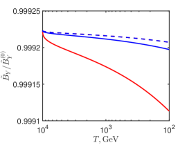
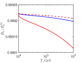
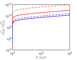
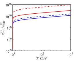
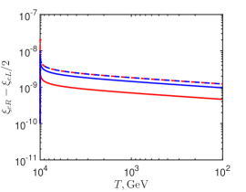
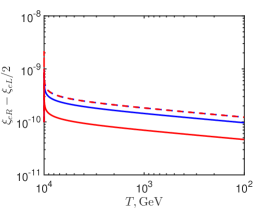
Figure 1: The evolution of the system at different $\tilde{B}_{\mathrm{Y}}^{(0)}$ and $q$ for the fixed $\tilde{k}_{\mathrm{max}}=10^{-3}$ based on the numerical solution of eq. (A). The initial condition is $\xi_{e\mathrm{R}}^{(0)}=10^{-10}$, $\xi_{e\mathrm{L}}^{(0)}=\xi_{0}^{(0)}=0$, and $\rho_{\mathrm{GW}}^{(c)}=0$ at $T_{\mathrm{RL}}=10\,\text{TeV}$. We account for the (H)MHD turbulence in solid lines, whereas the dashed ones are plotted without taking the turbulence into account. Red lines correspond to $\tilde{B}_{\mathrm{Y}}^{(0)}=1.4\times 10^{-1}$ and blue lines to $\tilde{B}_{\mathrm{Y}}^{(0)}=1.4\times 10^{-2}$. Panels (a) and (b): the evolution of the HMF; panels (c) and (d): the evolution of the energy density of GWs; cf. eqs. (2.15) and (A.8); panels (e) and (f): the evolution of the $\alpha$-dynamo parameter $\sim\xi_{e\mathrm{R}}-\xi_{e\mathrm{L}}/2$. In panels (a), (c), and (e), we set $q=1$; and panels (b), (d), and (f) correspond to $q=0.1$.

The HMF evolution depends on whether we account for the (H)MHD turbulence or not. The HMF evolution, without taking the (H)MHD turbulence into account, corresponds to $\eta_{\mathrm{eff}}=\sigma_{c}^{-1}$ and $\alpha_{\pm}=\alpha_{\mathrm{Y}}$ in eq. (3). The main contribution of the HMFs noise was mentioned in ref. [16] to result from $\eta_{\mathrm{eff}}$. Thus, the greater $\tilde{B}_{\mathrm{Y}}^{(0)}$ is, the faster HMF decays. This feature can be seen in figures 1 and 1. Red and blue dashed lines, plotted without the (H)MHD turbulence, overlap. It should be noted that, despite red solid lines are below blue ones, the absolute value of HMFs, shown in red, is almost one order of magnitude greater than of these depicted in blue in figures 1 and 1.

The evolution of the energy density of GWs $\rho_{\mathrm{GW}}^{(c)}$ in the cooling universe is shown in figures 1 and 1. First, greater $\tilde{B}_{\mathrm{Y}}^{(0)}$ leads to greater $\rho_{\mathrm{GW}}^{(c)}$; cf. red and blue solid lines in figures 1 and 1. Second, greater $\tilde{B}_{\mathrm{Y}}^{(0)}$ result in the faster decay of HMFs. Thus the energy density of GWs, which depends on $\tilde{B}_{\mathrm{Y}}$, will evolve slower for greater $\tilde{B}_{\mathrm{Y}}^{(0)}$. This feature can be also observed figures 1 and 1: the gap between solid and dashed lines in red is wider than between these in blue. Third, $\rho_{\mathrm{GW}}^{(c)}$ grows while the universe cools down and HMFs decays; cf. figures 1 and 1. It is a consequence of the cumulative effect of the integration over the conformal time in eq. (2).

The behavior of the $\alpha$-dynamo parameter $\alpha_{\mathrm{Y}}\sim\xi_{e\mathrm{R}}-\xi_{e\mathrm{L}}/2$ is depicted in figures 1 and 1. In fact, $\alpha_{\mathrm{Y}}$ is almost completely determined by the evolution of $\xi_{e\mathrm{R}}$ since $|\xi_{e\mathrm{L}}|\ll\xi_{e\mathrm{R}}$, as found in ref. [16].

One can see in figures 1 and 1 that $\alpha_{\mathrm{Y}}$ has a spike at $T\gtrsim T_{\mathrm{RL}}$. It can be explained by the backreaction of the hypermagnetic helicity on the asymmetries. Indeed, this spike results from the term $I_{\mathrm{H}}$ in eq. (A) for the asymmetry of right electrons $M_{\mathrm{R}}$. The level of the spike in higher for the greater initial helicity. This feature is seen in figures 1 and 1. The asymmetries fall down at greater evolution times because of the Higgs decays and especially the sphaleron process which acts on the asymmetry of left fermions. Taking into account the Higgs decays and the sphaleron process results in the nonconservation of the sum of the chiral imbalance and the (hyper-)magnetic helicity, which is usually conserved if only the Adler anomaly is considered. These processes are analogous to the spin-flip of fermions in electromagnetic plasma [28, 29]. The evolution of HMF in figures 1 and 1 does not reveal the spikes at $T\gtrsim T_{\mathrm{RL}}$ since it is dominated by the diffusion terms $\propto-2\tilde{k}^{2}\sigma_{c}^{-1}\tilde{\mathcal{E}}_{{\rm B_{\mathrm{Y}}}}$ in eq. (3).

The obtained behavior of HMFs can be explained if we calculate the typical scale of the HMFs instability. Using the results of ref. [30], one gets that

$$\tilde{k}_{\star}=\frac{\pi\sigma_{c}}{2\alpha^{\prime}}\left(\int_{0}^{\tilde{\eta}}\mathrm{d}\tilde{\eta}\xi_{e\mathrm{R}}\right)^{-1},$$ (4.1)

where we keep only the right asymmetry for simplicity. Equation (4.1) can be obtained, e.g., from the induction equation for HMF, $\partial_{\eta}\tilde{\mathbf{B}}_{\mathrm{Y}}=\alpha_{\mathrm{Y}}(\nabla\times\tilde{\mathbf{B}}_{\mathrm{Y}})+\dotsb$, where we keep only the instability term. Assuming the Chern-Simons wave distribution and using eq. (3.4), one gets that $\tilde{B}_{\mathrm{Y}}\propto\exp(\tilde{k}/\tilde{k}_{\star})$. A more careful derivation of $\tilde{k}_{\star}$ is provided in ref. [30].

One expects the HMF amplification if $\tilde{k}>\tilde{k}_{\star}$. The fast growth of $\xi_{e\mathrm{R}}$ to the value $\sim 10^{-8}$ takes place in the temperature range $\Delta T=T_{\mathrm{RL}}-T=10^{-1}\,\text{GeV}$ (see, e.g., figure 1 and ref. [16]). Thus we can estimate $\tilde{k}_{\star}\sim 10^{3}$, which is much greater than $\tilde{k}_{\mathrm{max}}=10^{-3}$ used in figure 1. It means that the diffusion is dominant in the HMF evolution. To trigger a sizable instability of HMFs in the considered system, one has to consider, e.g., a greater value of $\tilde{k}_{\mathrm{max}}\sim\tilde{k}_{\star}$. However, the condition of the plasma electroneutrality is violated even for $\tilde{k}_{\mathrm{max}}=0.1\sim\tilde{r}_{\mathrm{D}}^{-1}$.

The spectra of the hypermagnetic energy $R$ and the hypermagnetic helicity $H$ (see eq. (A)) at different plasma temperatures are depicted in figure 2. We show the initial spectra at $T=T_{\mathrm{RL}}$, which are Kolmogorov and depicted with dashed lines, and the spectra at EWPT. The spectra of seed fields evolve to the solid lines very rapidly. Therefore we do not show them for any intermediate temperatures.

The spectra at $T=T_{\mathrm{EW}}$ coincide with the seed ones, shown with dashed lines, for $\kappa\lesssim 10^{-5}$. For greater $\kappa$, the spectra start to decrease. This behavior is accounted for by the diffusion terms $\propto-\kappa^{2}$ in eq. (A). Thus, modes with greater $\kappa$ are damped more efficiently. This evolution of the HMFs is promising from the observational point of view since HMFs with large scales survive. Moreover, we can see in figure 2 that the spectra corresponding to a stronger seed field, shown with red color, start to decrease at smaller $\kappa$ compared to blue ones. It happens owing to the turbulence contribution to the effective diffusion coefficient. The above features justify our suggestion that the evolution of HMFs in this model is dominated by the diffusion.

The spectra at $T=T_{\mathrm{EW}}$ demonstrate the drastic change in their behavior when they drop below $\sim 10^{-20}$. This feature is related to the limited accuracy of numerical simulations. Thus, we can rely only on the part of the curves in figure 2 which are above $\sim 10^{-20}$.

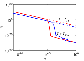
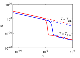
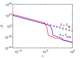
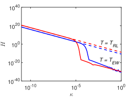
Figure 2: The spectra of the hypermagnetic energy $R$ and the hypermagnetic helicity $H$ versus the dimensioless wave vector $\kappa$ (see eq. (A)) for different $\tilde{B}_{\mathrm{Y}}^{(0)}$ and $q$, as well as the fixed $\tilde{k}_{\mathrm{max}}=10^{-3}$. The initial condition is the same as in figure 1. Here, we account for the (H)MHD turbulence. Dashed lines show the spectra of seed HMFs at $T=T_{\mathrm{RL}}$. Solid lines represent the situation when the universe cools down to EWPT. Red lines correspond to $\tilde{B}_{\mathrm{Y}}^{(0)}=1.4\times 10^{-1}$ and blue lines to $\tilde{B}_{\mathrm{Y}}^{(0)}=1.4\times 10^{-2}$. Panels (a) and (b): the spectra of the energy density; panels (c) and (d): the spectra of the hypermagnetic helicity; In panels (a) and (c), we set $q=1$; and panels (b) and (d) correspond to $q=0.1$.

The influence of the HMFs scale on the production of GWs is shown in figure 3, where we fix the strength of the seed HMF by $\tilde{B}_{\mathrm{Y}}^{(0)}=1.4\times 10^{-1}$ and vary $\tilde{k}_{\mathrm{max}}$. The effect of the (H)MHD turbulence on the evolution of HMFs was mentioned in refs. [16, 21] to be more sizable for small scale fields, i.e. for great $\tilde{k}_{\mathrm{max}}$. Thus HMFs, corresponding to greater $\tilde{k}_{\mathrm{max}}$ decay faster. It results in the slower enhancement of $\rho_{\mathrm{GW}}^{(c)}$ for such fields. Such a behavior is seen in figure 3 where red lines, with $\tilde{k}_{\mathrm{max}}=10^{-2}$, are below blue ones, with $\tilde{k}_{\mathrm{max}}=10^{-3}$. We can also see the negligible dependence on the initial hypermagnetic helicity; cf. figures 3 and 3.

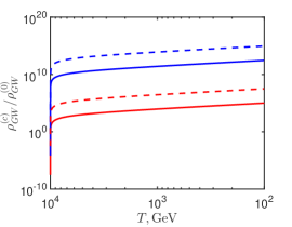
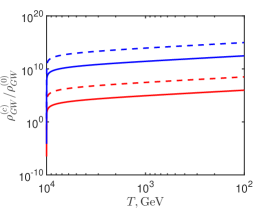
Figure 3: The evolution of the energy density of GWs at different $\tilde{k}_{\mathrm{max}}$ and $q$ for the fixed $\tilde{B}_{\mathrm{Y}}^{(0)}=1.4\times 10^{-1}$ based on the numerical solution of eq. (A). The initial condition is the same as in figure 1. We account for the (H)MHD turbulence in solid lines, wheres the dashed ones are plotted without taking the turbulence into account. Red lines correspond to $\tilde{k}_{\mathrm{max}}=10^{-2}$ and blue lines to $\tilde{k}_{\mathrm{max}}=10^{-3}$. (a) $q=1$; and (b) $q=0.1$.

The evolution of the system, shown in figures 1 and 3, qualitatively resembles the results obtained in ref. [14], where the generation of primordial GWs is driven by the CME. However, unlike ref. [14], where the turbulence was modeled fully numerically, we use a semi-analytical approach, which allows one to analyze the influence of different factors, like the strength of a seed HMF and its scale, on the production of GWs. Moreover, we study more realistic situation when the generation of relic GWs is driven by the lepton and Higgs asymmetries before EWPT. For this purpose, we utilize the analogs of the CME for the HMFs and of the Adler anomalies for the asymmetries.

4.1 Observability of relic GWs

Let us consider the possibility for the predicted GW signal to be observed with the current experimental techniques. For this purpose we take that $\tilde{B}_{\mathrm{Y}}^{(0)}=1.4\times 10^{-1}$, $\tilde{k}_{\mathrm{max}}=10^{-5}$, and $q=1$. The chosen $B_{\mathrm{Y}}^{(0)}=7\times 10^{26}\,\text{G}$ still does not violate the Big Bang nucleosynthesis constraint $B_{\mathrm{BBN}}=10^{11}\text{G}$ at $T_{\mathrm{BBN}}=0.1\,\text{MeV}$ [31]. The value of $\tilde{k}_{\mathrm{max}}$ is taken so that the HMFs noise is still noticeable but its influence is small (see solid and dashed lines in figure 4). The rest of the parameters is the same as in figure 1.

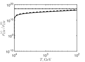
Figure 4: The energy density of GWs versus the plasma temperature for $\tilde{B}_{\mathrm{Y}}^{(0)}=1.4\times 10^{-1}$ ($B_{\mathrm{Y}}^{(0)}=7\times 10^{26}\,\text{G}$), $\tilde{k}_{\mathrm{max}}=10^{-5}$, and $q=1$. In the solid line, we account for the (H)MHD turbulence, whereas, in dashed one, not. The rest of the parameters and the initial condition are the same as in figure 1. The horizontal dash-dotted line is the averaged lower bound for the GW energy density, which can be experimentally probed presently.

One can see in the end of the solid line at $T=10^{2}\,\text{GeV}$ in figure 4 that the conformal energy density of GWs at $T_{\mathrm{EW}}$ is $\rho_{\mathrm{GW}}^{(c)}(T_{\mathrm{EW}})=5\times 10^{15}\rho_{\mathrm{GW}}^{(0)}=7.5\times 10^{-8}\,\text{eV}\cdot\text{cm}^{-3}$, where $\rho_{\mathrm{GW}}^{(0)}$ is given in eq. (A.8). We also assume that no other sources of GWs are after EWPT. Thus the current energy density of GWs is $\rho_{\mathrm{GW}}^{(\mathrm{now})}=\rho_{\mathrm{GW}}^{(c)}/a_{\mathrm{now}}^{3}=\rho_{\mathrm{GW}}^{(c)}(T_{\mathrm{EW}})$.

Some modern GWs detectors (see, e.g., ref. [32]) can potentially detect stochastic GWs with $\Omega\sim 10^{-10}$, where $\Omega=\tfrac{f\rho_{\mathrm{GW}}(f)}{\rho_{\mathrm{crit}}}$, $f=k/2\pi$ is the frequency of GWs in Hz, $\rho_{\mathrm{GW}}(f)$ is the spectrum of the energy density with respect to $f$, and $\rho_{\mathrm{crit}}=0.5\times 10^{-5}\,\text{GeV}\cdot\text{cm}^{-3}$ is the critical energy density of the universe. We can evaluate the total observable energy density as $\rho_{\mathrm{GW}}^{(\mathrm{obs})}\sim 3.1\times 10^{-6}\,\text{eV}\cdot\text{cm}^{-3}$, which is only $40$ times greater than the predicted value $\rho_{\mathrm{GW}}^{(\mathrm{now})}=7.5\times 10^{-8}\,\text{eV}\cdot\text{cm}^{-3}$. Thus, the GW background, described within our model, is potentially detectable using current GWs detectors after some enhancement of their sensitivity.

We can see in figure 4 that both the turbulent GW energy density, shown by the solid line, and the nonturbulent one, depicted by the dashed line, are below the observations threshold, represented by the dash-dotted line. The value of $(\rho_{\mathrm{GW}}^{(c)}/\rho_{\mathrm{GW}}^{(0)})_{\mathrm{obs}}=2.1\times 10^{17}$ corresponds to the sensitivity of, e.g., the NANOGrav experiment [32]. It corresponds to $\Omega\sim 10^{-10}.$

5 Conclusion

In this work, we have studied the production of relic GWs in turbulent plasma in the symmetric phase before the EWPT. Random HMFs, with the (H)MHD turbulence, are the driver for the GWs generation. HMFs are taken to couple to the gravity through their energy-momentum tensor. The evolution of HMFs in primordial plasma is governed by the analogs of the CME and the Adler anomalies in the presence of nonzero asymmetries of right and left electrons, left neutrinos, their antiparticles, as well as Higgs bosons.

We have used the realistic parameters and the initial condition of HMFs for the production of GWs. The same parameters, while utilized in the problem of the BAU generation (see, e.g., ref. [16]), result in BAU close to the observed value, $(\text{BAU})_{\mathrm{obs}}\sim 10^{-10}$. It is the advantage of our work compared to ref. [14], where the analogous problem, i.e. the generation of relic GWs driven by the CME, was studied. Moreover, we use the semi-analytical model, which is based on the (H)MHD turbulence [17, 20, 21]. It allows one to guess the dependence of the final results on the parameters of the system, in contrast to ref. [14], where purely numerical simulations were used.

In section 2, we have rederived eq. (2.5) for the tensor perturbations of the metric in the presence of HMFs. Then, using its formal solution in eq. (2.7), we have obtained the expression for the spectrum of the energy density of GWs in eq. (2) represented in conformal variables. After averaging and using the binary combinations of HMFs, such as their energy and the helicity, we get the final expressions for the energy density of GWs and its spectrum in eqs. (2.15) and (2).

Section 3 is devoted to the formulation of the dynamics of HMFs and the initial condition for them. Basically, it is similar to that in ref. [16], where we studied the BAU generation driven by turbulent HMFs. Such HMFs evolve owing to the analog of the CME in the presence of nonzero lepton asymmetries. We have also accounted for the backreaction of helical HMFs to the lepton asymmetries evolution because of the analog of the Adler anomalies for HMFs. The noise of HMFs is modeled by the analog of the (H)MHD turbulence. The main kinetic equations for the binary combinations of HMFs and the particle asymmetries are summarized in eqs. (3)-(3.4).

In section 4, we have presented the results of the numerical solution of the evolution eq. (3) and the energy density of GWs in eq. (2.15) basing on this solution. In figures 1 and 3, we have shown the strength of HMF $\tilde{B}_{\mathrm{Y}}$, the energy density of GWs $\rho_{\mathrm{GW}}^{(c)}$, and the $\alpha$-dynamo parameter $\sim\xi_{e\mathrm{R}}-\xi_{e\mathrm{L}}/2$ in the temperature range from $T=T_{\mathrm{RL}}=10\,\text{TeV}$ down to $T=T_{\mathrm{EW}}=10^{2}\,\text{GeV}$. We have analyzed the dependence of $\rho_{\mathrm{GW}}^{(c)}$ on the strength of the seed HMF $\tilde{B}_{\mathrm{Y}}^{(0)}$ for the fixed minimal scale $\tilde{k^{-1}}_{\mathrm{max}}$ (see figure 1), as well as on the minimal scale for the fixed strength of the seed HMF (see figure 3). There is a negligible dependence of $\rho_{\mathrm{GW}}^{(c)}$ on the initial helicity of HMFs. There results qualitatively resemble the findings of ref. [14].

We have briefly discussed the possibility to observe the predicted GWs background in section 4.1. Using the following realistic initial conditions: $B_{\mathrm{Y}}^{(0)}=7\times 10^{26}\,\text{G}$, $\tilde{k}_{\mathrm{max}}=10^{-5}$, $q=1$, $\xi_{e\mathrm{R}}^{(0)}=10^{-10}$, and $\xi_{e\mathrm{L}}^{(0)}=\xi_{0}^{(0)}=0$, we have obtained that the current energy density of GWs produced is only $\sim 40$ times below the threshold of the modern GWs detectors. Thus such a signal can be potentially observable in the nearest future.

In appendix A, we have rewritten the main expressions in the form adapted for numerical simulations.

Appendix A New variables

Following ref. [16], it is convenient to use the new variables in eq. (3),

$$\tilde{\mathcal{E}}_{{\rm B_{\mathrm{Y}}}}(\tilde{k},\tilde{\eta}) =\frac{\tilde{k}_{\mathrm{max}}\pi^{2}}{6\alpha^{\prime 2}}R(\kappa,\tau),\quad\tilde{\mathcal{H}}_{{\rm B_{\mathrm{Y}}}}(\tilde{k},\tilde{\eta})=\frac{\pi^{2}}{3\alpha^{\prime 2}}H(\kappa,\tau),$$

$$\xi_{\mathrm{R,L,0}}(\tilde{\eta}) =\frac{\pi\tilde{k}_{\mathrm{max}}}{\alpha^{\prime}}M_{\mathrm{R,L,0}}(\tau),\quad\tau=\frac{2\tilde{k}_{\mathrm{max}}^{2}}{\sigma_{c}}\tilde{\eta},\quad\tilde{k}=\tilde{k}_{\mathrm{max}}\kappa,$$ (A.1)

where $\kappa_{m}<\kappa<1$, $\kappa_{m}=\tilde{k}_{\mathrm{min}}/\tilde{k}_{\mathrm{max}}$, and $\tau\geq 0$ is the new dimensionless time. Using eq. (A), we rewrite eq. (3) in the form [16],

$$\frac{\partial R}{\partial\tau}= -\kappa^{2}\left(1+\lambda_{t}I_{\mathrm{R}}\right)R+\kappa^{2}\left(M_{\mathrm{R}}-\frac{M_{\mathrm{L}}}{2}-\lambda_{t}I_{\mathrm{H}}\right)H,$$

$$\frac{\partial H}{\partial\tau}= -\kappa^{2}\left(1+\lambda_{t}I_{\mathrm{R}}\right)H+\left(M_{\mathrm{R}}-\frac{M_{\mathrm{L}}}{2}+\lambda_{t}I_{\mathrm{H}}\right)R,$$

$$\frac{\mathrm{d}M_{\mathrm{R}}}{\mathrm{d}\tau}= I_{\mathrm{H}}-\left(M_{\mathrm{R}}-\frac{M_{\mathrm{L}}}{2}\right)I_{\mathrm{R}}-\Gamma^{\prime}(M_{\mathrm{R}}-M_{\mathrm{L}}+M_{0}),$$

$$\frac{\mathrm{d}M_{\mathrm{L}}}{\mathrm{d}\tau}= -\frac{1}{4}I_{\mathrm{H}}+\frac{1}{4}\left(M_{\mathrm{R}}-\frac{M_{\mathrm{L}}}{2}\right)I_{\mathrm{R}}-\Gamma^{\prime}(M_{\mathrm{L}}-M_{\mathrm{R}}-M_{0})/2-\frac{\Gamma^{\prime}_{s}}{2}M_{\mathrm{L}},$$

$$\frac{\mathrm{d}M_{0}}{\mathrm{d}\tau}= -\Gamma^{\prime}(M_{\mathrm{R}}+M_{0}-M_{\mathrm{L}})/2,$$ (A.2)

where

$$I_{\mathrm{R}}(\tau)= \int_{\kappa_{m}}^{1}\mathrm{d}\kappa^{\prime}R(\kappa^{\prime},\tau),\quad I_{\mathrm{H}}(\tau)=\int_{\kappa_{m}}^{1}\mathrm{d}\kappa^{\prime}\kappa^{\prime 2}H(\kappa^{\prime},\tau),\quad\lambda_{t}=\frac{2\sigma_{c}\tilde{k}_{\mathrm{max}}^{2}\pi^{2}}{9\alpha^{\prime 4}(\tilde{p}+\tilde{\rho})},$$

$$\Gamma^{\prime}(\tau)= \frac{121\sigma_{c}}{\tilde{\eta}_{\mathrm{EW}}\tilde{k}_{\mathrm{max}}^{2}}\left[1-\frac{T_{\mathrm{EW}}^{2}}{T_{\mathrm{RL}}^{2}}\left(1+\frac{T_{\mathrm{RL}}}{M_{0}}\frac{\sigma_{c}}{2\tilde{k}_{\mathrm{max}}^{2}}\tau\right)^{2}\right],$$ (A.3)

and $\Gamma^{\prime}_{s}=\sigma_{c}\Gamma_{\mathrm{sph}}/2\tilde{k}_{\mathrm{max}}^{2}$.

Equation (A) should be completed with the initial condition, which has the form,

$$R(\kappa,0)=C_{\mathrm{Y}}\kappa^{n_{\mathrm{Y}}},\quad H(\kappa,0)=q\frac{R(\kappa,0)}{\kappa},$$ (A.4)

where

$$C_{\mathrm{Y}}=\frac{3\alpha^{\prime 2}(1+n_{\mathrm{Y}})[\tilde{B}_{\mathrm{Y}}^{(0)}]^{2}}{\pi^{2}\tilde{k}_{\mathrm{max}}^{2}(1-\kappa_{m}^{1+n_{\mathrm{Y}}})}.$$ (A.5)

Equations (A)-(A.5) can be solved numerically.

The spectral density of GWs and their energy density in eqs. (2) and (2.15) should be also adapted to the new variables. The spectrum of the energy density is

$$\rho_{\mathrm{GW}}^{(c)}(\kappa,\tau)= \frac{\sigma_{c}^{2}\pi^{2}t_{\text{Univ}}^{2}T_{0}^{7}T_{\mathrm{RL}}^{2}G}{576\alpha^{\prime 4}\tilde{M}_{\mathrm{Pl}}^{2}\tilde{k}_{\mathrm{max}}}\frac{\tau}{\kappa^{3}}\int_{0}^{\tau}\frac{\mathrm{d}\tau^{\prime}}{(1+7.1\times 10^{-13}\tau^{\prime}/\tilde{k}_{\mathrm{max}})^{2}}$$

$$\times\iint_{S(\kappa)}\frac{\mathrm{d}\upsilon\mathrm{d}\varpi}{\upsilon{}^{3}\varpi^{3}}$$

$$\times\big{\{}[4\kappa^{2}\upsilon^{2}+(\kappa^{2}+\upsilon^{2}-\varpi^{2})^{2}][4\kappa^{2}\varpi^{2}+(\kappa^{2}-\upsilon^{2}+\varpi^{2})^{2}]R(\upsilon,\tau^{\prime})R(\varpi,\tau^{\prime})$$

$$+16\kappa^{2}\upsilon^{2}\varpi^{2}(\kappa^{2}+\upsilon^{2}-\varpi^{2})(\kappa^{2}-\upsilon^{2}+\varpi^{2})H(\upsilon,\tau^{\prime})H(\varpi,\tau^{\prime})\big{\}},$$ (A.6)

where $0<\kappa<2$ and $S(\kappa)$ is the 2D integration domain in the $(\upsilon,\varpi)$-plane. The energy density reads

$$\rho_{\mathrm{GW}}^{(c)}(\tau)= \int_{0}^{2k_{\mathrm{max}}}\rho_{\mathrm{GW}}^{(c)}(k,\tau)\mathrm{d}k=\rho_{\mathrm{GW}}^{(0)}\tau\int_{0}^{\tau}\frac{\mathrm{d}\tau^{\prime}}{(1+7.1\times 10^{-13}\tau^{\prime}/\tilde{k}_{\mathrm{max}})^{2}}$$

$$\times\int_{0}^{2}\frac{\mathrm{d}\kappa}{\kappa^{3}}\iint_{S(\kappa)}\frac{\mathrm{d}\upsilon\mathrm{d}\varpi}{\upsilon{}^{3}\varpi^{3}}$$

$$\times\big{\{}[4\kappa^{2}\upsilon^{2}+(\kappa^{2}+\upsilon^{2}-\varpi^{2})^{2}][4\kappa^{2}\varpi^{2}+(\kappa^{2}-\upsilon^{2}+\varpi^{2})^{2}]R(\upsilon,\tau^{\prime})R(\varpi,\tau^{\prime})$$

$$+16\kappa^{2}\upsilon^{2}\varpi^{2}(\kappa^{2}+\upsilon^{2}-\varpi^{2})(\kappa^{2}-\upsilon^{2}+\varpi^{2})H(\upsilon,\tau^{\prime})H(\varpi,\tau^{\prime})\big{\}},$$ (A.7)

where

$$\rho_{\mathrm{GW}}^{(0)}=\frac{\sigma_{c}^{2}\pi^{2}t_{\text{Univ}}^{2}T_{0}^{8}T_{\mathrm{RL}}^{2}G}{576\alpha^{\prime 4}\tilde{M}_{\mathrm{Pl}}^{2}}=1.5\times 10^{-23}\,\text{eV}\cdot\text{cm}^{-3}.$$ (A.8)

Equation (A) is used to plot figures 1, 1, 3, and 4 basing on the numerical solution, $R(\kappa,\tau)$ and $H(\kappa,\tau)$, of eq. (A).

References

[1]
LIGO Scientific collaboration and Virgo collaboration,
B.P. Abbott et al.,
Observation of gravitational waves from a binary black hole merger,
Phys. Rev. Lett.116 (2016) 061102
[arXiv:1602.03837].
[2]
LIGO Scientific collaboration and Virgo collaboration,
R. Abbott et al.,
GWTC-2: Compact Binary Coalescences Observed by LIGO and Virgo during the First Half of the Third Observing Run,
Phys. Rev. X11 (2021) 021053
[arXiv:2010.14527].
[3]
M. Bailes et al.,
Gravitational-wave physics and astronomy in the 2020s and 2030s,
Nat. Rev. Phys.3 (2021) 344.
[5]
J.D. Romano and N.J. Cornish,
Detection methods for stochastic gravitational-wave backgrounds: A unified treatment,
Living Rev. Relativity20 (2017) 2
[arXiv:1608.06889].
[6]
T. Regimbau,
The astrophysical gravitational wave stochastic background,
Res. Astron. Astrophys.11 (2011) 369 [arXiv:1101.2762].
[7]
C. Caprini and D.G. Figueroa,
Cosmological backgrounds of gravitational waves,
Class. Quantum Grav.35 (2018) 163001
[arXiv:1801.04268].
[8]
A. Kosowsky, A. Mack and T. Kahniashvili,
Gravitational radiation from cosmological turbulence,
Phys. Rev. D66 (2002) 024030
[astro-ph/0111483].
[9]
K. Fukushima, D.E. Kharzeev and H.J. Warringa,
The Chiral Magnetic Effect,
Phys. Rev. D78 (2008) 074033
[arXiv:0808.3382].
[10]
M.E. Peskin and D.V. Schroeder,
An Introduction to Quantum Field Theory,
Perseus Books, Reading, U.S.A. (1995), pp. 651–688.
[11]
M. Joyce and M. Shaposhnikov,
Primordial magnetic fields, right-handed electrons, and the Abelian anomaly,
Phys. Rev. Lett.79 (1997) 1193 [astro-ph/9703005].
[12]
M. Dvornikov and V. B. Semikoz,
Lepton asymmetry growth in the symmetric phase of an electroweak plasma
with hypermagnetic fields versus its washing out by sphalerons,
Phys. Rev. D87 (2013) 025023
[arXiv:1212.1416].
[13]
K. Kamada and A. Long,
Baryogenesis from decaying magnetic helicity,
Phys. Rev. D94 (2016) 063501
[arXiv:1606.08891].
[14]
A. Brandenburg, Y. He, T. Kahniashvili, M. Rheinhardt and J. Schober,
Relic gravitational waves from the chiral magnetic effect,
Astrophys. J.911 (2021) 110
[arXiv:2101.08178].
[15]
A.K. Pandey,
Gravitational waves in neutrino plasma and NANOGrav signal,
Eur. Phys. J. C81 (2021) 399
[arXiv:2011.05821].
[16]
M. Dvornikov and V.B. Semikoz,
Influence of the hypermagnetic field noise on the baryon asymmetry generation
in the symmetric phase of the early universe,
Eur. Phys. J. C81 (2021) 1001
[arXiv:2110.01071].
[17]
G. Sigl,
Cosmological magnetic fields from primordial helical seeds,
Phys. Rev. D66 (2002) 123002
[astro-ph/0202424].
[18]
S. Weinberg,
Cosmology,
Oxford University Press, New York, U.S.A. (2020), pp. 219–235.
[19]
L.D. Landau and E.M. Lifshitz,
The Classical Theory of Fields, seventh edition,
Nauka, Moscow, U.S.S.R. (1988), pp. 444–447.
[20]
L. Campanelli,
Evolution of magnetic fields in freely decaying magnetohydrodynamic turbulence,
Phys. Rev. Lett.98 (2007) 251302
[arXiv:0705.2308].
[21]
M. Dvornikov and V.B. Semikoz,
Influence of the turbulent motion on the chiral magnetic effect in the early Universe,
Phys. Rev. D95 (2017) 043538
[arXiv:1612.05897].
[22]
B.A. Campbell, S. Davidson, J. Ellis and K.A. Olive,
On the baryon, lepton-flavor and right-handed electron asymmetries of the universe,
Phys. Lett. B297 (1992) 118 [hep-ph/9302221].
[23]
D.S. Gorbunov, V.A. Rubakov,
Introduction to the Theory of the Early Universe: Hot Big Bang Theory,
World Scientific, Singapore (2011), p. 250.
[24]
I. Rogachevskii, O. Ruchayskiy, A. Boyarsky, J. Fröhlich, N. Kleeorin,
A. Brandenburg and J. Schober,
Laminar and turbulent dynamos in chiral
magnetohydrodynamics—I: Theory,
Astrophys. J.846 (2017) 153
[arXiv:1705.00378].
[25]
D.E. Kharzeev, J. Liao, S.A. Voloshin and G. Wang,
Chiral magnetic and vortical effects in high-energy nuclear collisions—A status report,
Prog. Part. Nucl. Phys. 88 (2016) 1 [arxiv:1511.04050].
[26]
A. Roper Pol, S. Mandal, A. Brandenburg, T. Kahniashvili and A. Kosowsky,
Numerical simulations of gravitational waves from early-universe turbulence,
Phys. Rev. D102 (2020) 083512
[arXiv:1903.08585].
[27]
P.A. Davidson,
Turbulence: An Introduction for Scientists and Engineers, second edition,
Oxford University Press, Oxford, UK (2015), p. 25.
[28]
M. Dvornikov,
Relaxation of the chiral imbalance and the generation of magnetic fields in magnetars,
J. Exp. Theor. Phys.123 (2016) 967
[arXiv:1510.06228].
[29]
A. Boyarsky, V. Cheianov, O. Ruchayskiy and O. Sobol,
Equilibration of the chiral asymmetry due to finite electron mass in electron-positron plasma,
Phys. Rev. D103 (2021) 013003
[arXiv:2008.00360].
[30]
V.B. Semikoz, A.Yu. Smirnov and D.D. Sokoloff,
Generation of hypermagnetic helicity and leptogenesis
in the early Universe,
Phys. Rev. D93 (2016) 103003
[arXiv:1604.02273].
[31]
B. Cheng, D.N. Schramm and J.W. Truran,
Constraints on the strength of a primordial magnetic field from Big Bang Nucleosynthesis,
Phys. Rev. D49 (1994) 5006 [astro-ph/9308041].
[32]
NANOGrav collaboration,
Z. Arzoumanian et al.,
The NANOGrav 12.5-year Data Set:
Search For An Isotropic Stochastic Gravitational-Wave Background,
Astrophys. J. Lett.905 (2020) L34
[arXiv:2009.04496].