Stability of large complex systems with heterogeneous relaxation dynamics

Abstract

We study the probability of stability of a large complex system of size $N$ within the framework of a generalized May model, which assumes a linear dynamics of each population size $n_{i}$ (with respect to its equilibrium value): $\frac{\mathrm{d}\,n_{i}}{\mathrm{d}t}=-a_{i}n_{i}-\sqrt{T}\sum_{j}J_{ij}n_{j}$. The $a_{i}>0$’s are the intrinsic decay rates, $J_{ij}$ is a real symmetric $(N\times N)$ Gaussian random matrix and $\sqrt{T}$ measures the strength of pairwise interaction between different species. Unlike in May’s original homogeneous model, each species has now an intrinsic damping $a_{i}$ that may differ from one another. As the interaction strength $T$ increases, the system undergoes a phase transition from a stable phase to an unstable phase at a critical value $T=T_{c}$. We reinterpret the probability of stability in terms of the hitting time of the level $b=0$ of an associated Dyson Brownian Motion (DBM), starting at the initial position $a_{i}$ and evolving in ‘time’ $T$. In the large $N\to\infty$ limit, using this DBM picture, we are able to completely characterize $T_{c}$ for arbitrary density $\mu(a)$ of the $a_{i}$’s. For a specific flat configuration $a_{i}=1+\sigma\frac{i-1}{N}$, we obtain an explicit parametric solution for the limiting (as $N\to\infty$) spectral density for arbitrary $T$ and $\sigma$. For finite but large $N$, we also compute the large deviation properties of the probability of stability on the stable side $T<T_{c}$ using a Coulomb gas representation.

1 Introduction

One of the main objectives in the study of large complex systems is to understand their stability properties. A major theoretical contribution to answer this hard question was made by Robert May in 1972 [1]. Using a simple ‘toy’ model May argued that large complex systems might become unstable as the system complexity (measured by the strength of interactions between different units) increases. The seminal work of May was motivated by ecological questions at his time [2], but even today his results have found resonance among the study of large complex systems arising across disciplines including economical sciences [3], neural networks [4, 5], gene regulations [6, 7] to cite a few. May’s approach will be discussed in detail below and consists in approximating the dynamics of the system by a set of linear coupled equations with random coefficients, and we refer to [8, 9, 10] for recent studies going beyond this linear approximation.

In his original toy model, May considered a complex system consisting of $N$ ecological species. To start with, each of the $N$ species is assumed to be in equilibrium with population $P_{i}^{*}$ ($i=1,2,\cdots,N$). Consider first the case where the species are non-interacting and linearly stable. By linearly stable, one means that if the population size $P_{i}$’s are slightly perturbed from their equilibrium values, then the deviation $n_{i}(t)=P_{i}(t)-P_{i}^{*}$ for each $i$ evolves in a deterministic manner as

$$\frac{\mathrm{d}n_{i}(t)}{\mathrm{d}t} =-n_{i}(t)\quad\text{for }i=1,\dots,N\,.$$ (1)

For simplicity, May assumed identical intrinsic decay rate (set to be unity in Eq. (1)) for each species, and this is what we call the homogeneous relaxation hypothesis. Imagine now switching on a pairwise interaction between the species, such that the dynamics is modified in the following way [1]

$$\frac{\mathrm{d}\,n_{i}(t)}{\mathrm{d}t} =-n_{i}(t)-\sqrt{T}\sum_{j}J_{ij}n_{j}(t)\quad\text{for }i=1,\dots,N\,\,,$$ (2)

where $J_{ij}$ represents a pairwise interaction term which denotes the influence of the $j^{th}$ species on the relaxation dynamics of the $i^{th}$ species and $\sqrt{T}$ is a measure of the strength of this interaction. The notation $\sqrt{T}$ for this interaction strength may seem a bit strange at this stage, but we will see later that $T$ will play the role of ’time’ in the associated Dyson Brownian motion picture. May’s further assumption was to model this complex interaction matrix $J_{ij}$ as a random Gaussian matrix with real elements. The dynamics for $\bm{n}(t)=(n_{1}(t),\dots,n_{N}(t))$ in Eq. (2) can be described in a compact matrix form as

$$\frac{\mathrm{d}\bm{n}(t)}{\mathrm{d}t} =-\left(\mathbf{I}+\sqrt{T}\,\mathbf{J}\right)\,\bm{n}(t)\,,$$ (3)

where $\mathbf{I}$ is the identity matrix and $\mathbf{J}$ is a real matrix with independent Gaussian entries. To make further progress, May also assumed that the interaction matrix $J_{ij}$ is symmetric. In that case, the random matrix $J_{ij}$ coincides with the Gaussian Orthogonal Ensemble (GOE) matrix in the Random Matrix Theory (RMT) literature [11, 12]. Note that for a GOE matrix $\mathbf{J}$ has the same distribution as $-\mathbf{J}$, hence we have chosen an overall negative sign in the interaction term in Eq. (2) without any loss of generality.

May’s equation (3) then maps a dynamics question “Is the multi-component system stable?” to a RMT question “Are all the eigenvalues of the random matrix $\mathbf{B}=\mathbf{I}+\sqrt{T}\,\mathbf{J}$ positive?”. Using the properties of GOE matrices, May argued that strictly in the large $N$ limit (where all finite size fluctuations disappear), there exists a critical strength $T_{c}$ where the system undergoes a stability-instability phase transition (sometimes known as May-Wigner transition): for $T<T_{c}$ the system is stable while for $T>T_{c}$ it is always unstable. Using the well-known Wigner semi-circular law for the average eigenvalue density of GOE eigenvalues as $N\to\infty$, May computed $T_{c}$ explicitly for this homogeneous model [1]. Thanks to the well-known properties of GOE matrices, one can go beyond May’s calculation of $T_{c}$ and even investigate the regime where $N$ is still large but finite and derive the behaviors of the typical and atypical fluctuations of the probability of stability of the system [13], as recalled briefly in the next section.

One of the important ingredients in May’s model (apart from the fact that $J_{ij}$ is a GOE matrix) was to assume a homogeneous decay rate for all species. In this paper, we address a simple question: assuming that $J_{ij}$ is still a GOE matrix, how the May-Wigner transition gets modified if one just makes the intrinsic decay rates for the species heterogeneous? This is a natural and simple generalization of May’s original toy model. In this heterogeneous version, one just replaces the identity matrix $\mathbf{I}$ in Eq. (3) with an arbitrary diagonal matrix with positive entries $\mathbf{A}=\mathrm{Diag}(a_{1},\dots,a_{N})$. Eq. (3) now gets modified to

$$\frac{\mathrm{d}\bm{n}(t)}{\mathrm{d}t} =-(\mathbf{A}+\sqrt{T}\,\mathbf{J})\bm{n}(t)=-\mathbf{B}\,\bm{n}(t)\,,$$ (4)

where the effective relaxation matrix

$$\mathbf{B} =\mathbf{A}+\sqrt{T}\mathbf{J}=\sqrt{T}\left[\mathbf{J}+\frac{1}{\sqrt{T}}\,\mathbf{A}\right]\,,$$ (5)

can be interpreted as a deformation of the GOE matrix $\mathbf{J}$ by an additive positive diagonal matrix $\mathbf{A}$, with $1/\sqrt{T}$ playing the role of the strength of ‘perturbation’. As the ‘time’ $T$ evolves, the matrix $\mathbf{B}$ evolves from its ‘initial’ value $\mathbf{A}$ and approaches a GOE matrix as $T\to\infty$. In May’s original homogeneous model where $\mathbf{A}=\mathbf{I}$, the matrix $\mathbf{B}$, for any strength parameter $\sqrt{T}$, is just a shifted GOE matrix. However, in the generic case $\mathbf{A}\neq\mathbf{I}$, the spectrum of $\mathbf{B}$ is more complex and is a continuous interpolation between the spectrum of the matrix $\mathbf{A}$ and the spectrum of the rescaled GOE matrix, as a function of increasing $T$. While deformed GUE (Gaussian unitary ensemble) models have been studied extensively in the recent past with many applications (see e.g. [14] and references therein), here we obtain a natural example of a deformed GOE matrix.

For this heterogeneous May model, we expect again that in the limit $N\to\infty$, where there are no finite size fluctuations, there should a critical value $T_{c}$ separating the stable ($T<T_{c}$) and the unstable ($T>T_{c}$) phases. However, it turns out that the moment the intrinsic diagonal positive rate matrix $\mathbf{A}$ differs from $\mathbf{I}$, computing $T_{c}$ becomes highly nontrivial. In this paper we first develop a general method to compute $T_{c}$ for arbitrary diagonal positive ${\mathbf{A}}$, and then use it to calculate $T_{c}$ explicitly for a particularly interesting case where the elements of $\mathbf{A}$ are distributed uniformly over a finite interval (we will refer to this case as the flat initial condition since this corresponds to the value of $\mathbf{B}$ at “time” $T=0$). This is the first main result of our paper.

Next, for a general positive diagonal matrix $\mathbf{A}$, computing the average density profile of the eigenvalues of the deformed matrix $\mathbf{B}$, for arbitrary $T$, is also hard. However, for the ‘flat initial condition’ described above, we are able to compute analytically the average density of the eigenvalues of $\mathbf{B}$ in the large $N$ limit for arbitrary $T$ (in explicit parametric form), providing our second main result.

Finally, for the same choice of $\mathbf{A}$ (the flat initial condition), we make the link with another ensemble, the deformed GUE, for which one can compute the joint density of eigenvalues for arbitrary $T$, going beyond just the average density. To the best of our knowledge, this provides a new RMT ensemble–a Coulomb gas in a harmonic potential, where the repulsive interaction between any pair of eigenvalues is a linear combination of logarithmic (as in the standard GUE) and log-sinh types. The RMT ensemble with only logarithmic (the standard GUE) or only log-sinh interaction [15, 16, 17, 18, 19, 20] have been studied before, but here we obtain naturally a linear combination of them as interaction. Such a mixed Coulomb gas is interesting to study in its own right. Moreover, this Coulomb gas approach also allows us to estimate, how for finite but large $N$, the probability of stability differs from $1$ on the stable side as one decreases $T$ below $T_{c}$ with $T_{c}-T\sim O(1)$ (we recall that strictly in the $N\to\infty$ limit, the probability of stability is exactly $1$ for $T<T_{c}$ by definition).

The rest of the paper is organized as follows: In Section 2, we recall in detail the derivation and properties of May’s original model. In particular, we describe in detail the finite size effects on the May-Wigner transition, in terms of the Tracy-Widom distribution and the large deviation functions describing respectively the typical and atypical fluctuations of the system. We then describe the new main model with heterogeneous relaxation dynamics. In Section 3, we describe the main tools to perform the study of the heterogeneous model: the resolvent, and its link with Dyson Brownian Motion (DBM) and the Burgers’ equation. This allows us to get the equation satisfied by the critical strength $T_{c}$ for a generic matrix $\mathbf{A}$. In Section 4, we show how one can get the parametric solution for the density, based again on the Burgers’ equation. In Section 5, we describe the deformed GUE with flat initial conditions and show how one can get the joint law density thanks to the Harish-Chandra-Itzykson-Zuber (HCIZ) integral. We then make the link with different models and show how one can get the large deviation function in the weakly stable phase for the original deformed GOE model with flat initial condition. Finally, we conclude in Section 6. Some details of the computation are relegated in the Appendices.

2 May’s homogeneous model and its heterogeneous generalization

2.1 May’s original homogeneous model

The homogeneous May model has already been described in the introduction. In this subsection, we show how $T_{c}$ for this model is computed in the strict $N\to\infty$ limit and then demonstrate how the probability of stability gets modified when $N$ is large, but finite. Also, this recapitulation would be useful for understanding the stability issues in the general setting of heterogeneous model that we will discuss in the next subsection.

The deviations $n_{i}(t)=P_{i}(t)-P_{i}^{*}$ evolve via Eq. (3) in the original homogeneous model, where $\mathbf{J}$ is a GOE matrix. Let us first briefly recall the properties of the GOE matrix. The entries of a GOE matrix are symmetric, $J_{ij}=J_{ji}$ and the independent entries are distributed via

$$\mathcal{P}_{N}(\mathbf{J})\mathrm{d}\mathbf{J} \propto\mathrm{exp}\left[-\frac{N}{4}{\rm Tr}\,\mathbf{J}^{2}\right]\mathrm{d}\mathbf{J}\,,$$ (6)

with $\mathrm{d}\mathbf{J}=\prod_{1\leq i\leq j\leq N}\mathrm{d}J_{ij}$ being the Lebesgue measure on the space of symmetric matrices. The eigenvalues $\{\lambda_{i}\}$ of $\mathbf{J}$ are all real, and it is well known [21] that the average density of eigenvalues,

$$\rho(x,N) =\frac{1}{N}\,\left\langle\sum_{i=1}^{N}\delta(\lambda_{i}-x)\right\rangle\,,$$ (7)

converges in the $N\to\infty$ limit towards the Wigner semi-circular distribution (see Fig. 1 (Left))

$$\rho(x,N\to\infty)\to\rho_{\mathrm{Wig}}(x) =\frac{1}{2\pi}\sqrt{4-x^{2}}\quad\text{for}\quad-2\leq x\leq 2\,.$$ (8)

As mentioned earlier, the joint density in Eq. (6) is manifestly invariant under the change $\mathbf{J}\to-\mathbf{J}$, so that $\mathbf{J}\overset{\text{in law}}{=}-\mathbf{J}$.

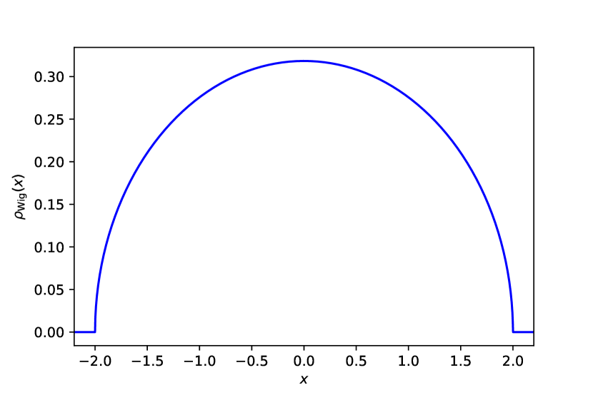
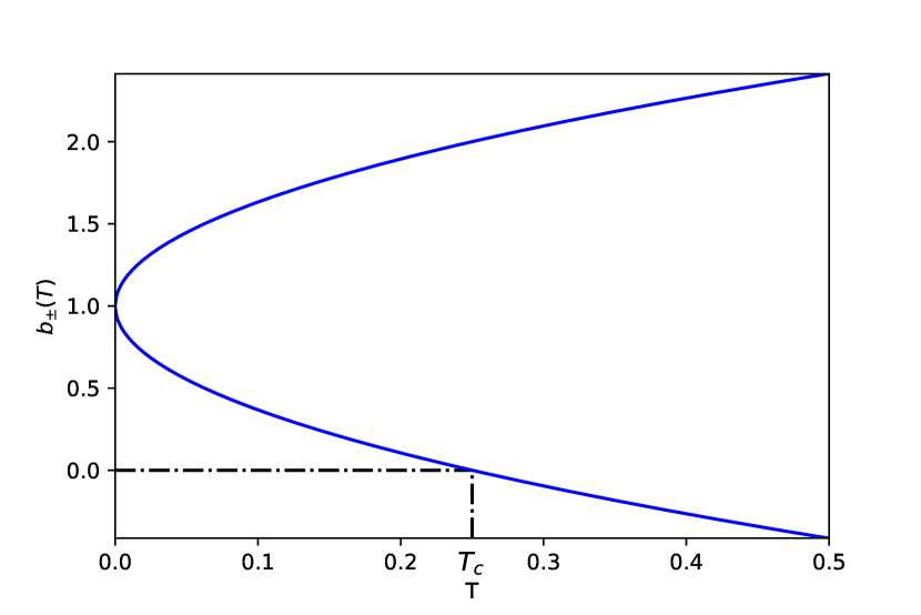
Figure 1: (Left) Plot of the Wigner semi-circular distribution in Eq. (8). (Right) Plot of the two edges $b_{\pm}(T)=1\pm 2\,\sqrt{T}$ of the limiting density of the eigenvalues of the matrix $\mathbf{B}=I+\sqrt{T}\,\mathbf{J}$ in Eq. (10), as a function of $T$. The critical strength occurs at $T_{c}=\frac{1}{4}$, where the lower edge $b_{-}(T)$ hits zero.

The matrix form of May’s equation (3) reads

$$\frac{\mathrm{d}\bm{n}(t)}{\mathrm{d}t} =-\mathbf{B}\,\bm{n}(t)\,,$$ (9)

where the effective relaxation matrix

$$\mathbf{B} =\mathbf{I}+\sqrt{T}\,\mathbf{J}\,,$$ (10)

is just a shifted GOE. Let $\lambda_{1}<\lambda_{2}<\ldots<\lambda_{N}$ and $b_{1}(T)<b_{2}(T)<\ldots<b_{N}(T)$ denote the ordered eigenvalues of $\mathbf{J}$ and $\mathbf{B}$ in Eq. (10) respectively. Clearly,

$$b_{i}(T) =1+\sqrt{T}\,\lambda_{i}(T)\,,\,\,{\rm for}\,{\rm all}\,i=1,2,\ldots,N\,.$$ (11)

One can now write down the condition for stability in terms of the ordered eigenvalues $\{b_{i}(T)\}$. From Eq. (9), it is clear that the system is stable if all eigenvalues of $\mathbf{B}$ are positive. Hence the probability of the stability can be expressed, for fixed $T$ and $N$, as

$$\mathcal{P}_{\mathrm{stable}}(T,N) =\mathrm{Prob}\left[b_{1}(T)>0,\dots,b_{N}(T)>0\right]\,,$$ (12)

or equivalently since we have ordered the eigenvalues

$$\mathcal{P}_{\mathrm{stable}}(T,N)=\mathrm{Prob}\left[b_{1}(T)>0\right] =\mathrm{Prob}\left[\lambda_{1}>-\frac{1}{\sqrt{T}}\right]\,,$$ (13)

where we used $b_{1}(T)=1+\sqrt{T}\,\lambda_{1}$ from Eq. (11). For finite $N$, the value of $\lambda_{1}$, and hence that of $b_{1}(T)=1+\sqrt{T}\,\lambda_{1}$ fluctuates from sample to sample. However, strictly in the $N\to\infty$ limit, we have seen before that the eigenvalues of $\mathbf{J}$ converge, almost surely, to Wigner semi-circular law in Eq. (8). This means that, as $N\to\infty$, all the eigenvalues $\{\lambda_{i}\}$ are supported within the finite interval $[-2,2]$. Since $\lambda_{1}$ is the lowest eigenvalue, it converges to the lower edge of the semi-circular, i.e., $\lambda_{1}\to-2$. Consequently, from Eq. (11), the eigenvalues $\{b_{i}(T)\}$ of $\mathbf{B}$ also converge to a shifted semi-circular law over the finite support $[b_{-}(T),b_{+}(T)]$ (see Fig. 1 (Right)), where

$$b_{-}(T) =1-2\,\sqrt{T}\quad{\rm and}\quad b_{+}(T)=1+2\,\sqrt{T}\,.$$ (14)

In particular, the lowest eigenvalue $b_{1}(T)$ converges to the lower edge as $N\to\infty$, i.e., $b_{1}(T)\to b_{-}(T)=1-2\,\sqrt{T}$. This means that as $N\to\infty$, almost surely, $b_{1}(T)>0$ if $T<T_{c}=1/4$ and $b_{1}(T)<0$ if $T>T_{c}=1/4$. Thus, the probability of stability in Eq. (13) also converges to an $N$-independent form as $N\to\infty$

$$\mathcal{P}_{\mathrm{stable}}(T,\infty) =\left\{\begin{array}[]{ll}1&\mbox{if }T<T_{c}=\frac{1}{4}\,,\\ 0&\mbox{otherwise.}\end{array}\right.$$ (17)

Thus, strictly in the $N\to\infty$ limit, the probability of stability, as a function of $T$, approaches a ‘sharp’ step function with the step located at $T_{c}=1/4$, as shown in Fig. 2.

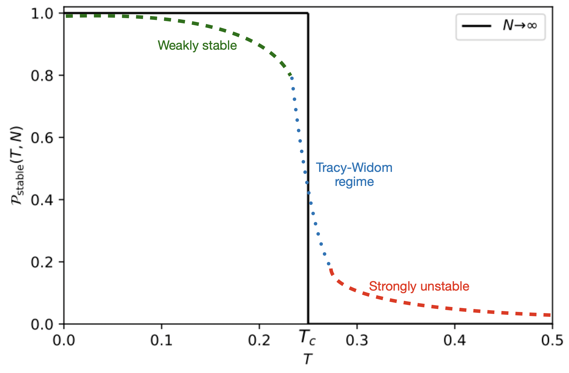
Figure 2: Sketch of the stability diagram in May’s homogeneous model: the probability of stability $\mathcal{P}_{\mathrm{stable}}(T,N)$ as a function of $T$ for fixed large $N$. The solid (black) line corresponds to the strictly $N\to\infty$ limit, where $\mathcal{P}_{\mathrm{stable}}(T,N)$ is a step function with the step at $T_{c}=1/4$. For finite but large $N$, this step function gets smoothened, as shown schematically by the dashed and dotted lines. The dotted line around $T_{c}$, shows the behavior of $\mathcal{P}_{\mathrm{stable}}(T,N)$ on a scale $|T-T_{c}|\sim O(N^{-2/3})$, and has the Tracy-Widom form. The dashed lines describe the behavior of $\mathcal{P}_{\mathrm{stable}}(T,N)$ when $|T-T_{c}|\sim O(1)$ and are described by the two large deviation behaviors on the two sides of $T_{c}$.

However, for finite but large $N$, this curve $\mathcal{P}_{\mathrm{stable}}(T,N)$ vs. $T$ will deviate from the step function (see Fig. 2). How does the step function get modified for finite but large $N$? To extract this information, we see from Eq. (13) that we need to know the probability distribution of the lowest (minimum) eigenvalue $\lambda_{1}$ of an $(N\times N)$ GOE matrix $\mathbf{J}$. Since for a Gaussian random matrix, the top eigenvalue $\lambda_{N}$ has the same distribution as $-\lambda_{1}$ by symmetry, we can equivalently express the probability of stability in Eq. (13) in terms of the distribution of the top eigenvalue $\lambda_{N}$ of the GOE matrix, namely

$$\mathcal{P}_{\mathrm{stable}}(T,N) =\mathrm{Prob}\left[b_{1}(T)>0\right]=\mathrm{Prob}\left[\lambda_{1}>-\frac{1}{\sqrt{T}}\right]=\mathrm{Prob}\left[\lambda_{N}<\frac{1}{\sqrt{T}}\right]\,.$$ (18)

Thus, we need to know how the top eigenvalue $\lambda_{N}$ of an $(N\times N)$ GOE matrix is distributed for finite but large $N$. At the time of May’s original work [1], this information was not available. Currently, however, one knows a great deal about the distribution of the top eigenvalue $\lambda_{N}$ of an $(N\times N)$ GOE matrix for finite but large $N$. This information was used to estimate $\mathcal{P}_{\mathrm{stable}}(T,N)$ for finite but large $N$ in Ref. [13], which we briefly recall below.

Summary of the large $N$ behavior of the top eigenvalue $\lambda_{N}$ of an $(N\times N)$ GOE matrix. As mentioned earlier, the largest eigenvalue $\lambda_{N}$ converges to $2$ as $N\to\infty$, i.e., coincides with the right edge of the Wigner semi-circular density in Eq. (8). However, for finite but large $N$, the random variable fluctuates around this right edge $2$. The scale of typical fluctuations is of order $O(N^{-2/3})$, where the probability distribution of $\lambda_{N}$, appropriately centered and scaled, is described by the celebrated Tracy-Widom (GOE) distribution [22, 23]. However, the Tracy-Widom form does not describe the large fluctuations of $\lambda_{N}$ of $O(1)$ around $2$ and they are described by two different large deviations form depending on whether $\lambda_{N}<2$ (left) [24, 25] or $\lambda_{N}>2$ (right) [26]. These three different regimes can be summarized by the following large $N$ behavior of the cumulative distribution ${\rm Prob}[\lambda_{N}<w]$

$$\mathrm{Prob}\left[\lambda_{N}<w\right] \approx\left\{\begin{array}[]{lll}\mathrm{exp}\left[-\frac{N^{2}}{2}\Psi_{-}(w)+o(N^{2})\right]&\mbox{for }w<2\mbox{ and }|w-2|\sim O(1)\,,\\ \\ \mathcal{F}^{(1)}\left(N^{2/3}(w-2)\right)&\mbox{for }|w-2|\sim O(N^{-\frac{2}{3}})\,,\\ \\ 1-\mathrm{exp}\left[-\frac{N}{2}\Psi_{+}(w)+o(N)\right]&\mbox{for }w>2\mbox{ and }|w-2|\sim O(1)\,.\end{array}\right.$$ (24)

The Tracy-Widom (GOE) function $\mathcal{F}^{(1)}(x)$ can be expressed as

$$\mathcal{F}^{(1)}(x) =\mathrm{exp}\left[-\frac{1}{2}\left(\int_{x}^{\infty}(s-x)q^{2}(s)+q(s)\mathrm{d}s\right)\right]\,.$$ (25)

where $q(s)$ is the Hasting-McLeod solution of the Painlevé II equation

$$q^{\prime\prime}(s) =2q^{3}(s)+sq(s)\quad\text{such that}\quad q(s)\underset{s\to\infty}{\sim}\mathrm{Ai}(s)\,.$$ (26)

The function $\mathcal{F}^{(1)}(x)$ has the leading order asymptotic behaviors

$$\mathcal{F}^{(1)}(x) =\left\{\begin{array}[]{ll}\mathrm{e}^{-\frac{1}{24}|x|^{3}+o(|x|^{3})}&,x\to-\infty\,,\\ \\ 1-\mathrm{e}^{-\frac{2}{3}|x|^{3/2}+o(x^{3/2})}&,x\to\infty\,.\end{array}\right.$$ (30)

The left and right large deviation functions, denoted respectively by $\Psi_{-}(w)$ and $\Psi_{+}(w)$ in Eq. (24), are also known explicitly [24, 25, 26] and read

$$\Psi_{-}(w) =\frac{1}{108}\left(72w^{2}-4w^{4}-(15\sqrt{2}w+2\sqrt{2}w^{3})\sqrt{2w^{2}+6}+27\left(\ln 18-2\ln\left(\sqrt{2}w+\sqrt{2w^{2}+6}\right)\right)\right)\,,\,\,w\leq 2$$ (31)

$$\Psi_{+}(w) =\frac{w\sqrt{w^{2}-4}}{2}-2\ln\frac{\sqrt{w^{2}-4}+w}{2}\,,\,\,\,w\geq 2.$$ (32)

The large deviation functions have the following asymptotic behaviors near the edge $w=2$:

$$\Psi_{-}(w) \propto(2-w)^{3}\mbox{ for }w\to 2\mbox{ and }w<2\,,$$ (33)

$$\Psi_{+}(w) \propto(w-2)^{\frac{3}{2}}\mbox{ for }w\to 2\mbox{ and }w>2\,.$$ (34)

One can check that these large deviation asymptotics as $w\to 2$ match smoothly with the Tracy-Widom tails in Eq. (30).

Large $N$ behavior of the probability of stability $\mathcal{P}_{\mathrm{stable}}(T,N)$ in the homogeneous May model. Using the relation in Eq. (18) one can then translate the large $N$ behavior of the cumulative density function (CDF) of the top eigenvalue ${\rm Prob}[\lambda_{N}<w]$ into the large $N$ behavior of $\mathcal{P}_{\mathrm{stable}}(T,N)$ in May’s homogeneous model. Setting $w=1/\sqrt{T}$ in Eq. (24), we see that the Wigner edge $w=2$ corresponds to $T_{c}=1/4$ and the behaviors of the probability of stability $\mathcal{P}_{\mathrm{stable}}(T,N)$ around $T_{c}=1/4$ for finite but large $N$ are described by

$$\mathcal{P}_{\mathrm{stable}}(T,N) \approx\left\{\begin{array}[]{lll}\mathrm{exp}\left[-\frac{N^{2}}{2}\Phi_{+}\left(T\right)+o(N^{2})\right]&\mbox{for }T>T_{c}=1/4\mbox{ and }|T-T_{c}|\sim O(1)\,,\\ \\ \mathcal{F}^{(1)}\left(N^{2/3}\left(T^{-1/2}-2\right)\right)&\mbox{for }|T-T_{c}|\sim O(N^{-\frac{2}{3}})\,,\\ \\ 1-\mathrm{exp}\left[-\frac{N}{2}\Phi_{-}\left(T\right)+o(N)\right]&\mbox{for }T<T_{c}=1/4\mbox{ and }|T-T_{c}|\sim O(1)\,,\end{array}\right.$$ (40)

where $\mathcal{F}^{(1)}(x)$ is the Tracy-Widom (GOE) function. The rate functions $\Phi_{\pm}(T)$ are given by:

$$\Phi_{\pm}(T) =\Psi_{\mp}\left(w=\frac{1}{\sqrt{T}}\right)\,,$$ (41)

with $\Psi_{\mp}$ given by Eqs. (31) and (32). These behaviors are schematically sketched by the dashed-dotted lines in Fig. 2 and describe precisely how the sharp step function (for $N\to\infty$) gets modified for finite but large $N$. In fact, the critical behavior around $T_{c}=1/4$ for finite $N$ in May’s homogeneous model is similar to the so called ‘double scaling’ limit in various matrix models arising in lattice gauge theory and they all share a ‘third order’ phase transition around the critical point, as reviewed extensively in Ref.  [13].

Let us remark that for finite but large $N$ and $T>T_{c}$, the probability of stability $\mathcal{P}_{\mathrm{stable}}(T,N)$ in Eq. (40) in the large deviation regime $T-T_{c}\sim O(1)$ deviates only very slightly $\sim\exp[-O(N^{2})]$ from its value $0$ when $N\to\infty$. Thus, the $N\to\infty$ ‘unstable’ phase remains ‘strongly’ unstable when $N$ reduces from $\infty$. Hence we refer to this phase as ‘strongly unstable’ in Fig. 2. In contrast, for $T<T_{c}$, the deviation of $\mathcal{P}_{\mathrm{stable}}(T,N)$ from its $N\to\infty$ value $1$ is of order $\sim\exp[-O(N)]$ which is much larger than the deviation $\sim\exp[-O(N^{2})]$ on the other side, i.e., for $T>T_{c}$. Thus, for $T<T_{c}$, the $N\to\infty$ ‘stable’ phase, where the system was stable with probability $1$ when $N\to\infty$, is likely to change with a relatively higher probability when $N$ is reduced from $\infty$. Hence, in Fig. 2, we refer to the phase $T<T_{c}$ as the ‘weakly stable’ phase.

Finally, we remark that these two different $N$ dependences of the large deviation behaviors of $\mathcal{P}_{\mathrm{stable}}(T,N)$ on either side of $T_{c}$ admits a nice physical interpretation in terms of the underlying log-gas picture of the eigenvalues of the relaxation matrix $\mathbf{B}=I+\sqrt{T}\,\mathbf{J}$, see Fig. 3. One can view the eigenvalues of the matrix $\mathbf{B}$ as a gas of $N$ particles living on the real line, confined by a harmonic potential and subject to a pairwise logarithmic repulsive interaction. For $T<T_{c}$, the system is asymptotically stable: this means all the eigenvalues $\{b_{i}(T)\}$ are above $0$ for $T<T_{c}$ with probability $1$ in the $N\to\infty$ limit. To reduce this probability from unity, i.e., to trigger an event that will make the system unstable for $T<T_{c}$, one needs a rare configuration of charges for which the lowest eigenvalue $b_{1}(T)<0$. This can be achieved by pulling the lowest eigenvalue $b_{1}(T)$ from its spectrum (whose lower edge is above $0$ for $T<T_{c}$) to the value $0$. This costs energy of order $O(N)$ since one needs to disturb (pull) only one eigenvalue, without disturbing the rest of the spectrum. Hence this explains the behavior $1-\mathcal{P}_{\mathrm{stable}}(T,N)\sim\exp[-O(N)]$ for $T<T_{c}$. In contrast, for $T>T_{c}$, the system is asymptotically unstable, i.e., the lower edge of the spectrum of eigenvalues $\{b_{i}(T)\}$ is already below $0$. To increase the stability, one needs to create a rare configuration where one pushes the whole gas of eigenvalues above $0$. Since this involves a re-arrangement of $N$ particles in the Coulomb gas, it will cost energy of $O(N^{2})$ (since each pair will contribute when the whole gas is compressed from its equilibrium configuration). This explains the behavior $\mathcal{P}_{\mathrm{stable}}(T,N)\sim\exp[-O(N^{2})]$ for $T>T_{c}$. This ‘pulled’ to ‘pushed’ phase transition occurs also in various lattice gauge models [27, 28, 29] where the ‘pulled’ phase corresponds to the ‘weak coupling’ phase in gauge theory, while the ‘pushed’ phase corresponds to the ‘strong coupling’ phase in gauge theory (for a review see [13]). Thus, the ‘stability-instability’ phase transition in May’s homogeneous model can also be viewed as a ‘pulled-pushed’ transition. The ‘stable’ phase in May’s model is the analogue of the ‘weak coupling’ phase of the gauge theory, while the ‘unstable’ phase is the analogue of the ‘strong coupling’ phase of the gauge theory  [13].

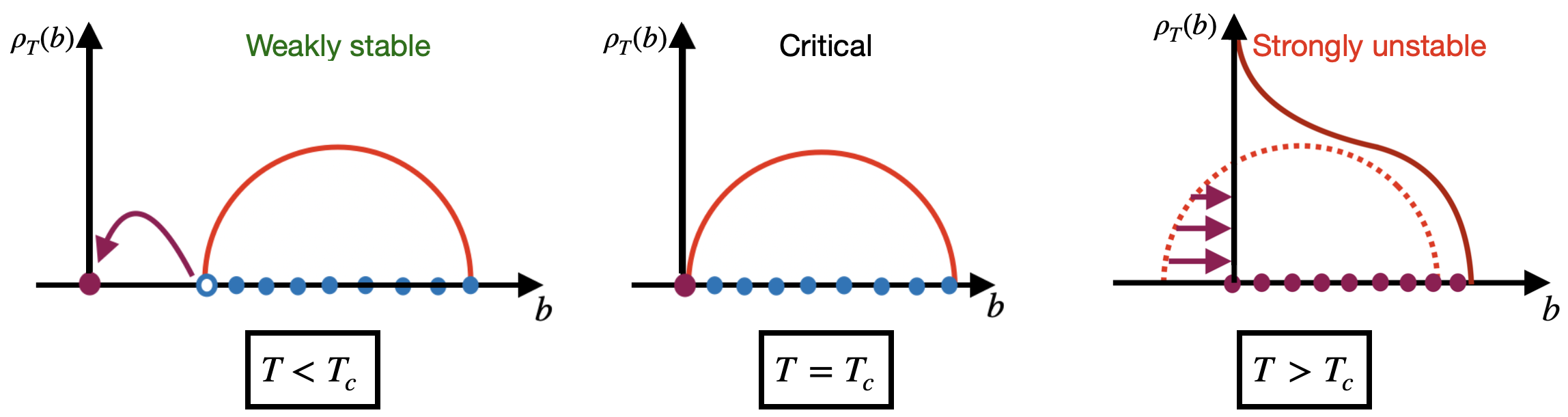
Figure 3: Sketch of the two different processes leading to the different scaling in $N$ of the probability in Eq. (40). (Left) For $T<T_{c}$, one needs to pull the lowest eigenvalue to the origin to make the system unstable, which does not change the equilibrium density. (Center) For $T=T_{c}$, the system is at the critical position where its lowest eigenvalue goes to $0$. (Right) For $T>T_{c}$, to make the system stable, one needs to push all eigenvalues above $0$. In this case, the gas rearranges itself and the equilibrium density is modified.

2.2 heterogeneous relaxation dynamics

A natural extension of May’s work is to drop the assumption that all the damping constants are equal and allow a spread in the distribution of the damping constants $a_{i}$’s, i.e., modify the evolution equation (2) to

$$\frac{\mathrm{d}\,n_{i}(t)}{\mathrm{d}t} =-a_{i}\,n_{i}(t)-\sqrt{T}\sum_{j}J_{ij}n_{j}(t)\quad\text{for }i=1,\dots,N\,\,,$$ (42)

where the $a_{i}>0$’s and are not necessarily equal. In the matrix form, this can be written as in Eq. (4) with $\mathbf{A}$ being a diagonal matrix with positive entries $\{a_{1},a_{2},\ldots,a_{N}\}$. To keep the model simple, we will still assume that the matrix $\mathbf{J}$ in Eq. (4) is a GOE matrix with density given in Eq. (6). Since we will first study this generalized system in the $N\to\infty$ limit, we assume the empirical distribution of the $a_{i}$’s converges to a continuous distribution $\mu(a)$ whose support is included in the positive real axis (since we have assumed the $a_{i}>0$ to ensure stability without interactions). Thus, $\mu(a)$ can be considered as the ‘initial’ value of the deformed GOE matrix $\mathbf{B}$ at $T=0$. The homogeneous May model corresponds to the choice of the ‘initial’ condition

$$\mu(a) =\delta(a-1)\,.$$ (43)

Our main goal, in this paper, is to understand how the May-Wigner transition may get modified when there is a spread or heterogeneity in the ‘initial’ density $\mu(a)$.

Starting from a given ‘initial’ density $\mu(a)$ at $T=0$, the eigenvalues $\{b_{i}(T)\}$ of $\mathbf{B}$ will evolve in ‘time’ $T$. The first natural question is: for a general ‘initial’ density $\mu(a)$, what is the limiting density $\rho_{T}(b)$ of the eigenvalues $\{b_{i}(T)\}$ at time $T$, in the $N\to\infty$ limit? For the special homogeneous initial condition in Eq. (43), we have seen in the previous subsection that $\rho_{T}(b)$ is a shifted semi-circular law with support over $b\in[1-2\,\sqrt{T},1+2\sqrt{T}]$ at ‘time’ $T$. For a general $\mu(a)$, we will again expect that the limiting density $\rho_{T}(b)$ will have a finite support $b\in[b_{-}(T),b_{+}(T)]$ at time $T$. If one can compute the location $b_{-}(T)$ of the lower edge of the support of the limiting density as a function of $T$, then setting $b_{-}(T=T_{c})=0$ will give us access to the exact critical strength $T_{c}$ for an arbitrary ‘initial’ condition $\mu(a)$.

Computing the limiting density $\rho_{T}(b)$ at $T$ for arbitrary ‘initial’ density $\mu(a)$ seems rather hard. However, one can make analytical progress for a specific choice of the ‘initial’ values $b_{i}(T=0)=a_{i}$,

$$a_{i} =1+\sigma\frac{i-1}{N}\quad\text{for }i=1,\dots,N\,,$$ (44)

which we call the flat initial condition since in the limit $N\to\infty$, the distribution of the $a_{i}$’s given by (44) converges towards the flat distribution $\mu(a)$ between $1$ and $1+\sigma$:

$$\mu(a) =\frac{1}{\sigma}\mathrm{\Pi}_{[1,1+\sigma]}(a)\,,$$ (45)

where $\Pi_{[a,b]}(x)$ is the indicator function: $\Pi_{[a,b]}(x)=1$ if $x$ is in $[a,b]$ and $0$ otherwise, see Fig. 4. The parameter $\sigma$ controls the width of this distribution and in particular the limit $\sigma\to 0$ corresponds to the homogeneous limit of May, so that we can consider this new model as one parameter extension of May’s original model.

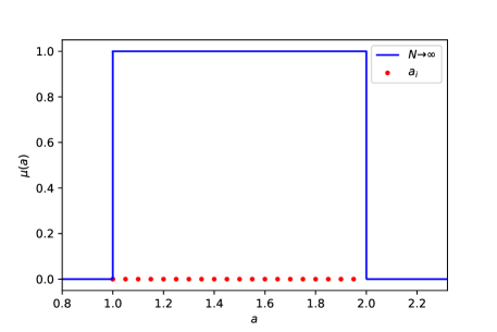
Figure 4: Flat discrete initial configuration (in red) of the $a_{i}$ with $N=20$ in Eq. (44) and their limiting flat density as $N\to\infty$ (in blue), for $\sigma=1$.

For this ‘flat initial condition’, we are able to compute, in the $N\to\infty$ limit, the limiting density $\rho_{T}(b)$ for all $T$. In particular, we will see in the next section that the precise knowledge of the lower edge $b_{-}(T)$ of its support will enable us to compute the exact value of $T_{c}$ in this model. Furthermore, for finite but large $N$, we expect that for the ‘flat initial condition’, the probability of stability $\mathcal{P}_{\mathrm{stable}}(T,N)$ near its critical point $T=T_{c}$ will have a qualitatively similar behavior as in its homogeneous counterpart in Eq. (40): In particular, from the general universality argument of the top eigenvalue of a GOE, we expect that the typical fluctuation of $\mathcal{P}_{\mathrm{stable}}(T,N)$ will still be described by the Tracy-Widom (GOE) scaling function $\mathcal{F}^{(1)}(x)$ in the middle line of Eq. (40). However, the large deviation functions in the region $|T-T_{c}|\sim O(1)$, respectively in the ‘unstable’ and the ‘stable’ side, are expected to be different in this heterogeneous ‘flat initial condition’ model. We will see in later sections that while we can compute the rate function on the ‘weakly stable’ side, i.e., for $T<T_{c}$, computing the rate function in the ‘strongly unstable’ phase remains a hard challenging problem even for the flat initial condition case.

3 Critical strength and the hitting time of a Dyson Brownian Motion

The idea to characterize the critical strength in the general setting is to think of the parameter $T$ as a (fictitious) ‘time’ variable of a well-known process called the Dyson Brownian Motion (DBM), described in Sec. 3.1. We can then obtain the time evolution of the associated resolvent, which satisfies the complex Burgers’ equation, see Sec. 3.2. Using the dynamics for the resolvent, we can derive in principle the critical strength $T_{c}$ for a general ‘initial’ density $\mu(a)$, see Sec. 3.3. For the special case of a ‘flat initial condition’, we derive $T_{c}$ explicitly in Sec. 3.3. Moreover, for this initial condition, the resolvent can be solved explicitly giving access to the full density $\rho_{T}(b)$, for arbitrary $T$, as discussed in the next section (Sec. 4).

3.1 Dyson Brownian Motion

From the joint law of the elements of the GOE matrix (6), by doing the change of variable in Eq. (10), we get the joint law of the elements $B_{ij}$ of the matrix $\mathbf{B}$,

$$\mathcal{P}_{N}(\mathbf{B})\mathrm{d}\mathbf{B} \propto\mathrm{exp}\left\{-N\,{\rm Tr}\,\left[\frac{(\mathbf{B}-\mathbf{A})^{2}}{4T}\right]\right\}\mathrm{d}\mathbf{B}\,,$$ (46)

with $\mathrm{d}\mathbf{B}=\prod_{1\leq i\leq j\leq N}\mathrm{d}B_{ij}$. Since $\mathbf{A}$ is diagonal, this can be equivalently written as:

$$\mathcal{P}_{N}(\mathbf{B})\mathrm{d}\mathbf{B} \propto\prod_{i=1}^{N}\mathrm{exp}\left[-\frac{N}{4T}(B_{ii}-a_{i})^{2}\right]\mathrm{d}B_{ii}\prod_{j:j>i}\mathrm{exp}\left[-\frac{N}{2T}B_{ij}^{2}\right]\mathrm{d}B_{ij}\,.$$ (47)

Under this form, one recognizes the propagator of the Brownian motion for a particle starting at time $T=0$ at the position $x_{0}$ and evaluated at time $T$:

$$\mathcal{P}\left(x,T|x_{0},0\right) =\mathrm{exp}\left[-\frac{1}{4DT}(x-x_{0})^{2}\right]\,,$$ (48)

with the diffusion constant $D=\frac{1}{N}$. Under this framework, we can naturally interpret the strength parameter $T$ as a time variable: each element of the matrix $\mathbf{B}$ evolves according to a Brownian motion until time $T$, starting at $a_{i}$ for the diagonal element $B_{ii}$ and starting at $0$ for the off-diagonal elements. At each instant $T$, one can diagonalize the matrix $\mathbf{B}$ and obtain its eigenvalues $\{b_{i}(T)\}$ which are real. It is then natural to ask how these eigenvalues $\{b_{i}(T)\}$ evolve with time $T$. Using a second order perturbation theory as in quantum mechanics, Dyson [30] showed that they follow what is now known as the ($\beta=1$) Dyson Brownian Motion (DBM), namely

$$\frac{\mathrm{d}b_{i}(T)}{\mathrm{d}T} =\frac{1}{N}\sum_{j:j\neq i}\frac{1}{b_{i}(T)-b_{j}(T)}+\sqrt{2D}\,\eta_{i}(T)\,,$$ (49)

starting from the initial condition,

$$b_{i}(0) =a_{i}\,.$$ (50)

In Eq. (49), $\eta_{i}(T)$, for each $i$, is an independent Gaussian white noise with zero mean and correlator $\langle\eta_{i}(t)\eta_{j}(t^{\prime})\rangle=\delta_{ij}\,\delta(t-t^{\prime})$. The trajectory of a $\beta=1$ DBM, evolving with $T$, is represented in Fig. 5 (Left). As Dyson did, one can redo the computation for Hermitian and symplectic matrices $\mathbf{J}$. For each case (symmetric/Hermitian/symplectic), one gets again the dynamics (49), with a diffusion constant $D=\frac{1}{N\beta}$, where $\beta=1,2,4$ is the Dyson index characterizing these three standard ensembles of Gaussian matrices. In particular the case $\beta=2$ will be useful later which also corresponds to the dynamics of $N$ vicious walkers, or non-intersecting Brownian motions, see [29, 31, 32, 33, 34]. For large $N$, one can therefore interpret the critical value $T_{c}$ as the hitting time of the barrier at $b=0$ of such a DBM, when the lower edge $b_{-}(T)$ hits the level $0$, see Fig. 5 (Left). One then needs first to compute the lower edge $b_{-}(T)$ of the DBM in the large $N$ limit and then compute the critical strength (or time) by setting

$$b_{-}(T_{c}) =0\,.$$ (51)

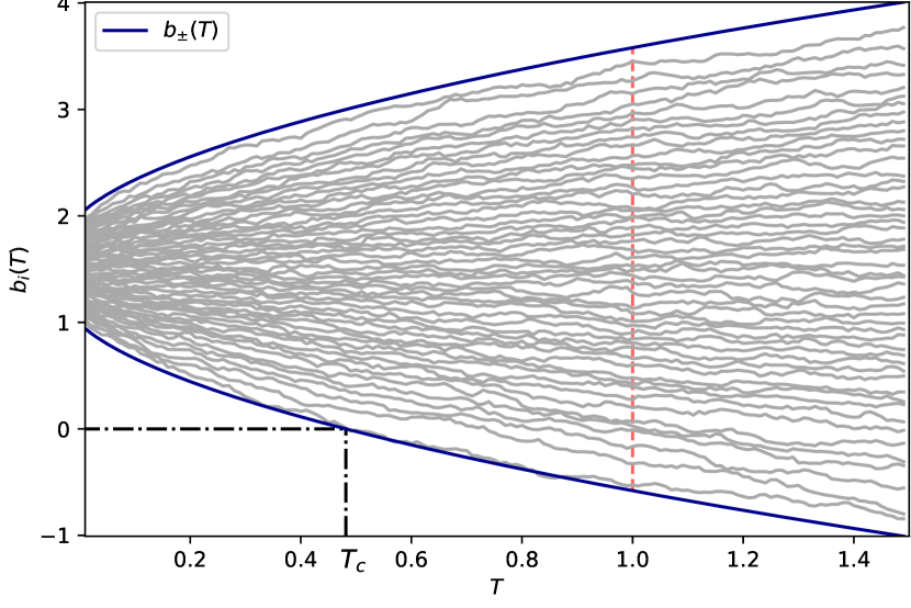
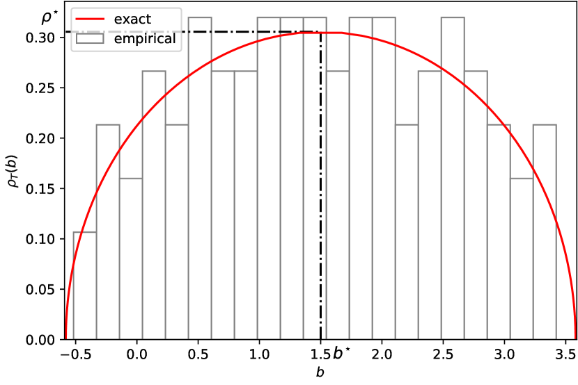
Figure 5: (Left) A representation of the DBM described by Eq. (49) at $\beta=1$ with the initial flat condition (44) for $\sigma=1$ and $N=50$. In blue, the limiting curve for the bottom and top edges as $N\to\infty$. The dotted line corresponds to the value of $T=1$ of the plot of the limiting density in the right. (Right) Plot of the limiting density for the flat initial density using the parametric solution (109) for $\sigma=T=1$, compared to a histogram of the positions of the DBM at this time.

3.2 The resolvent and the complex Burgers’ equation

The main tool to perform the computation of the edges of an evolving density of eigenvalues $\{b_{i}(T)\}$ via Eq. (49) is to introduce the resolvent, a key transform in RMT. The derivation of the properties of the resolvent needed in this section are recalled in the Appendices. For $z\in\mathbb{C}$ and $z\neq b_{i}(T)$ the resolvent is defined by

$$g_{N}(z,T) =\frac{1}{N}{\rm Tr}\,(z\,\mathbf{I}-\mathbf{B})^{-1}=\frac{1}{N}{\rm Tr}\,\left(z\,\mathbf{I}-\mathbf{A}-\sqrt{T}\mathbf{J}\right)^{-1}=\frac{1}{N}\sum_{i=1}^{N}\frac{1}{z-b_{i}(T)}\,.$$ (52)

In the large $N\to\infty$ limit, the sum is replaced by an integral, defined for all $z$ in the complex plane outside the support $[b_{-}(T),b_{+}(T)]$ of the density on the real axis,

$$g(z,T) =g_{\infty}(z,T)=\int_{b_{-}(T)}^{b_{+}(T)}\frac{\rho_{T}(b)}{z-b}\mathrm{d}b\,,$$ (53)

with $\rho_{T}(b)$ denoting the limiting density of the DBM at time $T$. From the knowledge of a resolvent, one gets the corresponding density, using the Socochi-Plemelj formula (see Appendix A.1),

$$\rho_{T}(b) =\frac{1}{\pi}\mathfrak{Im}\,g(b-\mathrm{i}0^{+},T)\,,$$ (54)

where $\mathfrak{Im}$ denotes the imaginary part. The lower and the upper edges $b_{\mp}(T)$ of the density $\rho_{T}(b)$ can be extracted from the resolvent $g(z,T)$ by applying the following general prescriptions (see Appendix A.3 for the derivation).

• First, define the inverse function $z(\mathrm{g})$ of the resolved $g(z)$, i.e., $z(g(z))=z$. We have suppressed the $T$ dependence of $g(z,T)$ for convenience. For example, for the semi-circular density in Eq. (8), the resolvent $g(z)=(z\pm\sqrt{z^{2}-4})/2$ is well known. Its inverse function is then $z(\mathrm{g})=\mathrm{g}+1/\mathrm{g}$.

• Next, find the roots of $z^{\prime}(\mathrm{g})=0$ where $z^{\prime}(\mathrm{g})=dz(\mathrm{g})/d\mathrm{g}$. In general, this equation will have multiple roots. For a density confined in a single interval on the real line, this has typically two roots, denoted by $g_{*}$ (the lower one) and $g^{*}$ (the upper one). For example, for the semi-circular distribution, $z^{\prime}(\mathrm{g})=1-1/\mathrm{g}^{2}=0$ gives two roots $\mathrm{g}_{*}=-1$ and $\mathrm{g}^{*}=1$. The smallest root is $\mathrm{g}_{*}=-1$ and the largest one is $\mathrm{g}^{*}=1$.

• The lower edge $b_{-}(T)$ of the support of the density is then given by

  $$b_{-}(T) =z(\mathrm{g}_{*})\,,$$ (55)

  Similarly, the upper edge of the support is given by the other root, i.e., $b_{+}(T)=z(\mathrm{g}^{*})$. For example, for the semi-circular law, one gets $b_{-}=-2$ and $b_{+}=2$ which indeed are respectively the lower and the upper edge of the support $[-2,2]$ of the density in Eq. (8).

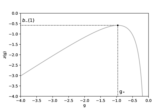
Figure 6: Representation of the inverse function $z(\mathrm{g})$ of the resolvent $g(z,T)$ for $T=\sigma=1$. If one starts from the origin $g=0$ and goes to the left, the function $z(\mathrm{g})$ increases until it reaches the point $g_{*}$ from which one can get the lower edge $b_{-}(1)\approx-0.580457$.

Next, one needs to find the equation of motion describing the resolvent from which we can get the lower edge by Eq. (55). Since the resolvent in Eq. (52) is a functional of the positions of particles evolving according to the DBM (49), the idea is to apply Ito’s lemma in Eq. (49) to get the stochastic evolution for the resolvent. Taking the limit $N\to\infty$ the noise term vanishes and one can show that $g(z,T)$ is the solution of the complex inviscid Burgers’ equation [35, 36],

$$\partial_{T}g(z,T)+g(z,T)\partial_{z}g(z,T) =0\,,$$ (56)

evolving from the initial condition $g(z,0)=g_{0}(z)=\int\mathrm{d}a\frac{\mu(a)}{z-a}$. Using the method of characteristics, see for example Sec. 3 of [34], the solution can be expressed in a parametric form as

$$g(z,T) =g_{0}(\xi)\,,$$ (57)

with

$$\xi =z-Tg_{0}(\xi)\,.$$ (58)

For $z$ and $T$ fixed and given $g_{0}$, one first needs to solve Eq. (58) for $\xi$ and then inject the solution in Eq. (57). Conversely, from Eq. (58) with $\xi$ fixed, one can express $z$ as an implicit function of $\xi$

$$z(\xi) =\xi+Tg_{0}(\xi)\,.$$ (59)

The idea would be to eliminate $\xi$ from Eqs. (57) and (59) to obtain $g(z,T)$ as a function of $z$ for fixed $T$. However, in practice, this is not always easy, as we will see shortly.

3.3 Critical strength

We now have all the necessary ingredients to compute the critical strength $T_{c}$. Since the lower edge is given by Eq. (55), we need to first solve $z^{\prime}(\mathrm{g})=0$ and find its lowest root, see Fig. 6 for an illustration. The equation $z^{\prime}(\mathrm{g})=0$ is equivalent to

$$\frac{\mathrm{d}z(\xi)}{\mathrm{d}\xi}\frac{\mathrm{d}\xi}{\mathrm{d}g} =0\,.$$ (60)

In general the term $\frac{\mathrm{d}\xi}{\mathrm{d}g}$ is non-zero, hence this is equivalent to solve

$$\frac{\mathrm{d}z(\xi)}{\mathrm{d}\xi} =0\,.$$ (61)

Using the expression (59) for $z(\xi)$, one gets

$$1+Tg^{\prime}_{0}\left(\xi_{*}(T)\right) =0\,,$$ (62)

where $\xi_{*}(T)$ denotes the lowest root of Eq. (62). Injecting this $\xi_{*}(T)$ back into Eq. (59) and using Eq. (55) gives the lower edge

$$b_{-}(T) =\xi_{*}(T)+T\,g_{0}\left(\xi_{*}(T)\right)\,,$$ (63)

where $\xi_{*}(T)$ is obtained from Eq. (62). Finally, setting $b_{-}(T_{c})=0$ gives $T_{c}$.

To summarize, we have again the following large $N\to\infty$ behavior of the probability of stability with arbitrary initial density $\mu(a)$,

$$\mathcal{P}_{\mathrm{stable}}(T,\infty) =\left\{\begin{array}[]{ll}1&\mbox{if }T<T_{c}\,,\\ 0&\mbox{otherwise.}\end{array}\right.$$ (66)

where now the critical strength $T_{c}$, which implicitly depends on $\mu(a)$, is obtained from the solution of the transcendental equation

$$\xi_{*}(T_{c})+T_{c}\,g_{0}\left(\xi_{*}(T_{c})\right) =0\,,$$ (67)

with $\xi_{*}(T_{c})$ is given in Eq. (62). Our algorithm for determining $T_{c}$, for arbitrary initial density $\mu(a)$, thus follows three principal steps:

• Given $\mu(a)$, we first determine the initial resolvent $g_{0}(z)=\int\mathrm{d}a\frac{\mu(a)}{z-a}$.

• Once we have $g_{0}(z)$, we solve Eq. (62) and determine $\xi_{*}(T)$.

• Next we inject this $\xi_{*}(T)$ in the transcendental equation (67) and solve it to determine $T_{c}$.

For example, in May’s original homogeneous model, we have $\mu(a)=\delta(a-1)$. This gives, $g_{0}(z)=1/(z-1)$. Substituting this in Eq. (62), we get two roots, and the lowest root gives $\xi_{*}(T)=1-\sqrt{T}$. Substituting this in Eq. (67) gives $1-2\sqrt{T_{c}}=0$, and hence $T_{c}=1/4$. Our method, outlined above, holds for arbitrary $\mu(a)$ and in the next subsection, we show that for the flat initial condition with $\mu(a)$ given in Eq. (45), the general procedure described above can be carried out explicitly, thus providing a nontrivial generalization of May’s homogeneous initial condition.

Critical strength for the flat initial condition: As a nontrivial example, we now consider the flat initial condition with $\mu(a)$ given in Eq. (45). In this case, the initial resolvent is given by:

$$g_{0}(z) =\frac{1}{\sigma}\int_{1}^{1+\sigma}\frac{\mathrm{d}a}{z-a}=\frac{1}{\sigma}\ln\left(\frac{z-1}{z-1-\sigma}\right)\,,$$ (68)

and its derivative is given by

$$g_{0}^{\prime}(z) =-\frac{1}{(z-1)(z-1-\sigma)}\,.$$ (69)

Using Eq. (62), $\xi_{*}(T)$ satisfies the quadratic equation

$$\left(\xi_{*}(T)-1)\right)\left(\xi_{*}(T)-1-\sigma\right) =T\,,$$ (70)

whose lowest solution is given by

$$\xi_{*}(T) =1+\frac{\sigma}{2}-\frac{\sigma}{2}\sqrt{1+\frac{4T}{\sigma^{2}}}\,.$$ (71)

Using Eq. (63), the lower edge at fixed $T$ is given by

$$b_{-}(T) =1+\frac{\sigma}{2}-\frac{\sigma}{2}\sqrt{1+\frac{4T}{\sigma^{2}}}+\frac{T}{\sigma}\ln\frac{\sqrt{1+\frac{4T}{\sigma^{2}}}-1}{1+\sqrt{1+\frac{4T}{\sigma^{2}}}}\,.$$ (72)

Setting $b_{-}(T_{c})=0$ in Eq. (72) gives $T_{c}$. However, it is not easy to solve explicitly this transcendental equation. To proceed further, we first write Eq. (72) in a more compact form,

$$b_{-}(T) =1-\sigma h\left(\frac{4T}{\sigma^{2}}\right)\,,$$ (73)

where the scaling function $h(u)$ is given by

$$h(u) =\frac{\sqrt{1+u}-1}{2}+\frac{u}{2}\,\ln\left(\frac{1+\sqrt{u+1}}{\sqrt{u}}\right)\,.$$ (74)

This function admits the following asymptotic behaviors near the origin and at infinity:

$$h(u) \sim\left\{\begin{array}[]{ll}\frac{1}{4}\left(1+2\ln 2-\ln u\right)u&\mbox{for }u\to 0\,,\\ \\ \sqrt{u}-\frac{1}{2}+\frac{1}{6}u^{-\frac{1}{2}}&\mbox{for }u\to\infty\,.\end{array}\right.$$ (78)

Setting $b_{-}(T_{c})=0$ in Eq. (73) gives

$$h\left(\frac{4T_{c}}{\sigma^{2}}\right) =\frac{1}{\sigma}\,.$$ (79)

Hence we can write

$$T_{c}(\sigma) =\frac{\sigma^{2}}{4}u\left(\frac{1}{\sigma}\right)\,,$$ (80)

where $u(h)$ is the inverse function of $h(u)$. Since the function $h(u)$ is explicit in Eq. (74), its inverse function $u(h)$ can be easily plotted. Thus, we can plot $T_{c}$ in Eq. (80) as a function of the spread $\sigma$, as shown in Fig. 7. The asymptotic behaviors of $T_{c}$ for small and large $\sigma$ can also be derived using Eq. (78) and are given by

$$T_{c}(\sigma) \sim\left\{\begin{array}[]{ll}\frac{1+\sigma}{4}&\mbox{for }\sigma\to 0\,,\\ \\ \frac{\sigma}{\ln\left(\frac{\sigma}{4}\right)}&\mbox{for }\sigma\to\infty\,.\end{array}\right.$$ (84)

In particular, we recover as expected the limit $T_{c}=\frac{1}{4}$ of May’s original model for $\sigma\to 0$. In the limit $\sigma\to\infty$, we find $T_{c}\to\infty$ from Eq. (84), which indicates that for large $\sigma$, the system is always stable, regardless of the value of the strength parameter $T$. This is an interesting result which perhaps could not have been guessed a priori.

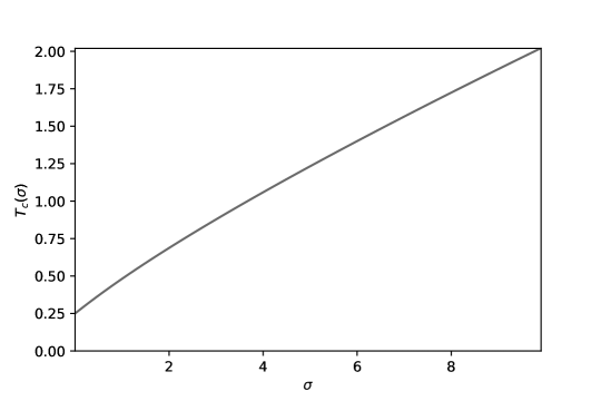
Figure 7: Plot of the critical strength $T_{c}$ given in Eq. (80), as a function of the spread $\sigma$.

4 Parametric solution for the density with flat initial condition

The goal of this section is to obtain an expression for the limiting density $\rho_{T}(b)$ of the eigenvalues of the matrix $\mathbf{B}$ for the flat initial condition (44), at arbitrary time $T$. The idea is to rely again on the complex Burgers’ equation (56) for the resolvent. As we will see, the density $\rho_{T}(b)$ cannot be easily expressed in terms of known analytical functions. However, it can be expressed in an easily plottable parametric form.

We start with the two basic equations satisfied by the resolvent $g(z,T)$, namely the solution of the complex Burger’s equation in Eq. (57) and Eq. (59). For easy reading, let us re-write these two equations together

$$g(z,T) =g_{0}(\xi)$$ (85)

$$z(\xi) =\xi+T\,g_{0}(\xi)\,.$$ (86)

The idea is to eliminate the auxiliary variable $\xi$ between these two equations and express $g$ as a function of $z$, for a fixed $T$.

To proceed, we start with the initial resolvent

$$g_{0}(\xi) =\int\frac{\,\mu(a)}{\xi-a}\mathrm{d}a\,.$$ (87)

Suppose we could invert this equation and write $\xi$ as a function of $g_{0}$

$$\xi =z_{0}(g_{0}(\xi))\,.$$ (88)

Thus $z_{0}(.)$ is just the inverse function of $g_{0}(\xi)$ in Eq. (87). Substituting Eq. (85) in Eq. (88) gives

$$\xi =z_{0}(g(z,T))\,.$$ (89)

Using this relation in Eq. (86) and further using $g_{0}(\xi)=g(z,T)$, Eq. (86) reduces to

$$z =T\,g(z,T)+z_{0}(g(z,T))\,.$$ (90)

Thus, for fixed $T$, if we know the initial inverse function $z_{0}(.)$, we have, in principle, a closed equation for $g(z,T)$. From the expression (68) of the initial resolvent $g_{0}$ in the flat initial condition case, its inverse function $z_{0}(g)$ is given by:

$$z_{0}(g) =1+\sigma+\frac{\sigma}{\mathrm{e}^{\sigma g}-1}\,,$$ (91)

Substituting this in Eq. (90), we then have a closed equation for the resolvent $g(z,T)$ at any time $T$

$$z =T\,g(z,T)+1+\sigma+\frac{\sigma}{\mathrm{e}^{\sigma g(z,T)}-1}\,.$$ (92)

Solving explicitly $g(z,T)$ from this transcendental equation does not seem feasible, unfortunately. To derive the density $\rho_{T}(b)$ from this resolvent $g(z,T)$ using Eq. (54), we set $z=b-\mathrm{i}0^{+}$, with $b$ between the two edges $b_{\pm}(T)$. Then by Eq. (54) we have $g(b-\mathrm{i}0^{+},T)=u+\mathrm{i}\pi\rho$, where $u$ is the real part of the resolvent. For simplicity, we have used the shorthand notation $u\equiv u(b,T)$ and $\rho\equiv\rho_{T}(b)$. Identifying the real and the imaginary parts of (92), we get a pair of coupled equations

$$\left\{\begin{array}[]{ll}b&=1+\sigma+Tu+\sigma\,\mathfrak{Re}\left[\dfrac{1}{\mathrm{e}^{\sigma(u+\mathrm{i}\pi\rho)}-1}\right]\,,\\ 0&=T\pi\rho+\sigma\,\mathfrak{Im}\left[\dfrac{1}{\mathrm{e}^{\sigma(u+\mathrm{i}\pi\rho)}-1}\right]\,.\\ \end{array}\right.$$ (95)

One can multiply the numerator and denominator inside the brackets by $\mathrm{e}^{\sigma(u-\mathrm{i}\pi\rho)}-1$, to get the real and imaginary parts of the function inside the brackets, and the system can then be written as

$$\left\{\begin{array}[]{ll}b&=1+\sigma+Tu+\sigma\dfrac{\cos(\sigma\pi\rho)\mathrm{e}^{\sigma u}-1}{\mathrm{e}^{2\sigma u}-2\cos(\pi\sigma\rho)\mathrm{e}^{\sigma u}+1}\,,\\ 0&=T\pi\rho-\sigma\dfrac{\sin(\pi\sigma\rho)\mathrm{e}^{\sigma u}}{\mathrm{e}^{2\sigma u}-2\cos(\pi\sigma\rho)\mathrm{e}^{\sigma u}+1}\,.\\ \end{array}\right.$$ (98)

Ideally, the goal would be to eliminate $u$ from these pair of equations and express $\rho\equiv\rho_{T}(b)$ as a function of $b$, for fixed $T$. Let us first consider the simple case of May’s homogeneous model, i.e., the limit $\sigma\to 0$. In this limit, Eq. (98) reduces to

$$\left\{\begin{array}[]{ll}b&=1+Tu+\frac{u}{u^{2}+\pi^{2}\,\rho^{2}}\,,\\ \\ 0&=T\pi\rho-\frac{\pi\,\rho}{u^{2}+\pi^{2}\,\rho^{2}}\,.\\ \end{array}\right.$$ (102)

Eliminating $u$ from these pair of equations, one immediately gets the shifted Wigner semi-circular density

$$\rho_{T}(b){\Large{|}}_{\sigma=0} =\frac{1}{2\pi T}\,\sqrt{4T-(b-1)^{2}}\,,$$ (103)

supported over the interval $b\in\left[1-2\,\sqrt{T},1+2\,\sqrt{T}]\right]$. Thus, in May’s homogeneous model, starting from the initial condition $\mu(a)=\delta(a-1)$, the density of eigenvalues $b_{i}(T)$’s, at any time $T>0$, is of the shifted Wigner semi-circular form in Eq. (103).

For general $\sigma>0$, eliminating $u$ from Eq. (98) and expressing $\rho_{T}(b)$ explicitly (as in the $\sigma=0$ case) seems difficult. Instead, for a general $\sigma>0$, one can obtain the solution parametrically as follows. We note that the top equation of (98) is a parametric expression for $b(u,\rho)$. The idea is to eliminate the dependency on $u$ by working a bit on the bottom equation of (98). To do so, let us denote by $w=\mathrm{e}^{\sigma u}$, and then from the bottom equation of (98) $w$ satisfies a quadratic equation,

$$\frac{w^{2}}{2}-w\left(\frac{\sigma^{2}}{2T}\mathrm{{\rm sinc}missing}(\pi\sigma\rho)+\cos(\pi\sigma\rho)\right)+\frac{1}{2} =0\,,$$ (104)

where $\mathrm{sinc}(x)=\frac{\sin(x)}{x}$ is the standard sinus cardinal function. Let us introduce further the function

$$f_{\sigma,T}(\rho) =\frac{\sigma^{2}}{2T}\mathrm{{\rm sinc}missing}\left(\pi\sigma\rho\right)+\cos\left(\pi\sigma\rho\right)\,,$$ (105)

plotted in Fig. 8 (Left).

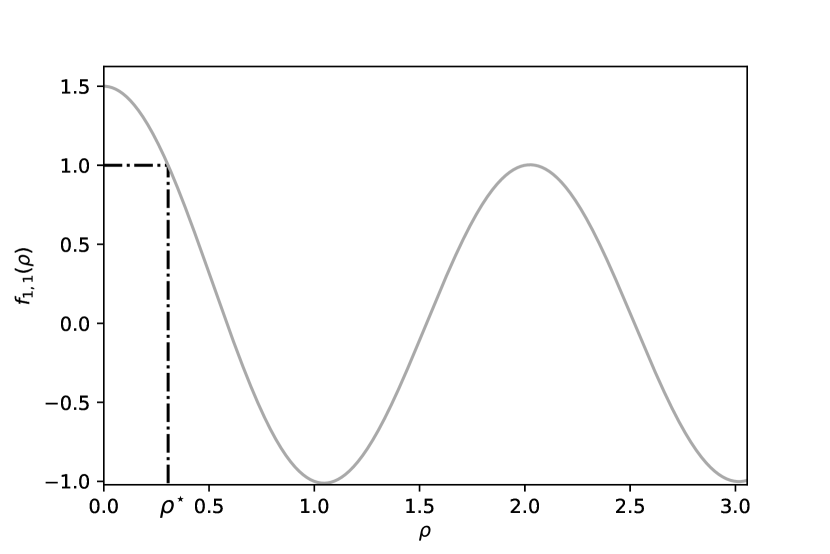
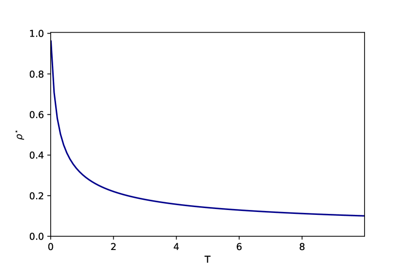
Figure 8: (Left) Plot of $f_{\sigma,T}(\rho)$ given in Eq. (105), as a function of $\rho$ for $\sigma=T=1$. Only the part on the left of the value $\rho^{\star}\approx 0.305637$ contribute to the parametric solution of the density. (Right) Plot of the maximum $\rho^{\star}$ described by Eq. (111) as a function of $T$, for $\sigma=1$.

Let us now imagine that the value of $\rho$ is fixed. Then the two solutions $w_{\pm}(\rho)$ of the system (104) are given in terms of this function $f_{\sigma,T}(\rho)$ by,

$$w_{\pm}(\rho) =f_{\sigma,T}(\rho)\pm\sqrt{f_{\sigma,T}(\rho)^{2}-1}\,,$$ (106)

and they satisfy the symmetry relation

$$\frac{1}{w_{-}(\rho)} =w_{+}(\rho)\,.$$ (107)

Injecting this into the top equation of (95) we get two solutions $b_{\pm}(\rho)$:

$$b_{\pm}(\rho) =1+\frac{\sigma}{2}+\frac{T}{\sigma}\ln w_{\pm}(\rho)+\frac{T}{2\sigma\,{\rm sinc}(\pi\sigma\rho)}\left(w_{\pm}-\frac{1}{w_{\pm}}\right)\,.$$ (108)

Using the symmetry relation (107) and the expression (106) for $w_{\pm}(\rho)$, we get the following parametric solution for the density

$$b_{\pm}(\rho) =1+\frac{\sigma}{2}\pm\frac{T}{\sigma}\left(\ln\left(f_{\sigma,T}(\rho)+\sqrt{f_{\sigma,T}(\rho)^{2}-1}\right)+\frac{\sqrt{f_{\sigma,T}(\rho)^{2}-1}}{{\rm sinc}\left(\pi\sigma\rho\right)}\right)\,.$$ (109)

In Fig. 9, we plot the two branches $b_{\pm}(\rho)$ as a function of $\rho$ for fixed $T$. Indeed, if one rotates this plot anticlockwise by $\pi/2$ and then reflects around the vertical axis, one gets the desired density $\rho_{T}(b)$ as a function of $b$, as seen in Fig. 5 (Right). Apart from being able to plot the density, one can also extract a few additional information from the explicit expression in Eq. (109), as discussed below.

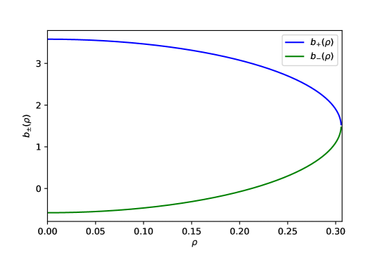
Figure 9: Plot of the two inverse functions $b_{\pm}(\rho)$ given in Eq. (108), for $\sigma=T=1$. Rotating the figure anticlockwise, followed by a reflection around the vertical axis, gives $\rho_{T}(b)$ as a function of $b$, as shown in Fig. 5 (Right).

Maximum value of the density: From Eq. (109), we see that the maximum value of the density $\rho^{\star}$ is attained at the point $b^{\star}$ for which $b_{+}(\rho)=b_{-}(\rho)$, i.e., $b^{\star}=1+\frac{\sigma}{2}$. The value of the maximum of the density $\rho^{\star}=\rho_{T}\left(b^{\star}\right)$, is therefore given as the first positive solution of

$$f_{\sigma,T}(\rho^{\star}) =1\,,$$ (110)

which using Eq. (105) is equivalent to finding the first positive solution of

$$\rho^{\star}\tan\left(\frac{\sigma\pi\rho^{\star}}{2}\right) =\frac{\sigma}{2T\pi}\,.$$ (111)

A plot of the maximum $\rho^{\star}$ as a function of $T$ for $\sigma=1$ is given in Fig. 8 (Right).

Behavior near the edges: By Taylor expanding the function $b_{\pm}(\rho)$ near $\rho=0$, we have

$$b_{\pm}(\rho) \sim b_{\pm}(T)\mp\frac{T\pi^{2}}{2}\sqrt{\sigma^{2}+4T}\,\rho^{2}\quad\mbox{ as }\rho\to 0\,,$$ (112)

where the edges $b_{\pm}(T)$ are given by

$$b_{\pm}(T) =1+\frac{\sigma}{2}\pm\left[\frac{\sigma}{2}\,\sqrt{1+\frac{4T}{\sigma^{2}}}+\frac{T}{\sigma}\,\ln\left(1+\frac{\sigma^{2}}{2T}+\frac{\sigma^{2}}{2T}\,\sqrt{1+\frac{4T}{\sigma^{2}}}\right)\right]\,.$$ (113)

It is easy to verify that the expression for $b_{-}(T)$ coincides with Eq. (72). Inverting the relation in Eq. (112), one finds that the density vanishes as a square root near the edge, with a prefactor that can be computed explicitly

$$\rho_{T}(b) \sim\frac{1}{\pi}\sqrt{\frac{2}{T}}\frac{1}{(\sigma^{2}+4T)^{\frac{1}{4}}}\sqrt{(b_{\pm}(T)-b)_{+}}\quad\mbox{ as }b\to b_{\pm}(T)\,.$$ (114)

where $(x)_{+}$ is equal to $x$ for $x>0$ and $0$ otherwise.

5 The deformed GUE with flat initial condition and the left large deviation function of the dynamical system

So far, we have computed the average density of eigenvalues $\rho_{T}(b)$ in the large $N$ limit of the relaxation matrix, $\mathbf{B}=\mathbf{A}+\sqrt{T}\,\mathbf{J}$ for any $T$, where $J$ is an $N\times N$ GOE matrix and $\mathbf{A}$ is diagonal with positive entries drawn from a flat distribution over $[1,1+\sigma]$ with width $\sigma$. This gives us the exact $T_{c}$ between the stable to unstable transition. We expect that for finite but large $N$, the probability of stability will have a qualitatively similar behavior as in the homogeneous model in Eq. (40), see also Fig. 2:

$$\mathcal{P}_{\mathrm{stable}}(T,N) \approx\left\{\begin{array}[]{lll}\mathrm{exp}\left[-\frac{N^{2}}{2}\Phi_{+}(\sigma,T)+o(N^{2})\right]&\mbox{for }T>T_{c}\mbox{ and }|T-T_{c}|\sim O(1)\,,\\ \\ \mathcal{F}^{(1)}\left(\gamma N^{2/3}\left(T^{-1/2}-T_{c}^{-1/2}\right)\right)&\mbox{for }|T-T_{c}|\sim O(N^{-\frac{2}{3}})\,,\\ \\ 1-\mathrm{exp}\left[-\frac{N}{2}\Phi_{-}(\sigma,T)+o(N)\right]&\mbox{for }T<T_{c}\mbox{ and }|T-T_{c}|\sim O(1)\,,\end{array}\right.$$ (120)

where $\gamma$ is a constant of order one and and the large deviation functions $\Phi_{\pm}(\sigma,T)$ on either sides of $T_{c}$ would be different. Note that for $\sigma=0$, the large deviation functions $\Phi_{\pm}(T)=\Phi_{\pm}(\sigma=0,T)$ could be related to the cumulative distribution of the top eigenvalue $\lambda_{N}$ of the matrix $\mathbf{J}$, see Eq. (41). However for $\sigma>0$, there is no such relation and one needs to compute $\Phi_{\pm}(\sigma,T)$ from first principles. It turns out (see later) that to compute the large deviation functions $\Phi_{\pm}(\sigma,T)$, we need the information on the full joint distribution of eigenvalues, and not just the one point function, i.e., the average density.

Hence, our next natural step was to see if we could compute the joint distribution of the eigenvalues of $\mathbf{B}$, where $\mathbf{J}$ is a GOE matrix. Unfortunately, we did not succeed yet in that. However, it turns out that one can compute the joint distribution of eigenvalues in a Hermitian counterpart of the relaxation matrix, $\tilde{\mathbf{B}}=\mathbf{A}+\sqrt{T}\tilde{\mathbf{J}}$, where $\mathbf{A}$ is still diagonal with a flat distribution, but now $\mathbf{J}$ is Hermitian, i.e., a GUE matrix.

In this section, for this deformed GUE model, we derive an explicit formula for the joint law of eigenvalues for the flat initial condition, thanks to the Itzykson-Zuber determinantal formula. We will see that this leads to a new Coulomb gas, where the eigenvalues can be interpreted as the positions of a gas of particles confined in a harmonic potential and repelling pairwise as in the standard GUE, but with an additional twist that the pairwise interaction here is a linear combination of a logarithmic (as in standard GUE) and a log-sinh type interaction. Finally, using this Hermitian modification, we will show how to compute at least the large deviation function $\Phi_{-}(\sigma,T)$ appearing in Eq. (120), in the ‘weakly stable’ phase ($T<T_{c}$) in the original deformed GOE model. However, computing the large deviation function $\Phi_{+}(\sigma,T)$ on the ‘strongly unstable’ phase ($T>T_{c}$) still remains out of reach.

5.1 The deformed GUE with flat initial condition and its joint law for the eigenvalues

The deformed GUE model [37, 38, 39, 14] is the Hermitian counterpart of the deformed GOE model

$$\tilde{\mathbf{B}} =\mathbf{A}+\sqrt{T}\tilde{\mathbf{J}}\,,$$ (121)

with the matrix $\mathbf{A}={\rm Diag}(a_{1},\dots,a_{N})$ with positive entries as before. The matrix $\tilde{\mathbf{J}}$ is a GUE matrix whose law is given by:

$$\mathcal{P}_{N}(\tilde{\mathbf{J}})\mathrm{d}\tilde{\mathbf{J}} =\mathrm{exp}\left[-N{\rm Tr}\,\frac{\tilde{\mathbf{J}}^{2}}{2}\right]\mathrm{d}\tilde{\mathbf{J}}\,,$$ (122)

with now $\mathrm{d}\tilde{\mathbf{J}}=\prod_{i=1}^{N}\mathrm{d}\tilde{J}_{ii}\prod_{j>i}\mathrm{d}\mathfrak{Re}\tilde{J}_{ij}\,\mathrm{d}\mathfrak{Im}\tilde{J}_{ij}$, the Lebesgue measure on the space of Hermitian matrices. One can repeat the second perturbation theory analysis for the eigenvalues and shows that they follow the $\beta=2$ DBM (49), with diffusion constant $D=1/(2N)$. In the large $N$ limit, we get the same Burgers’ equation (56) for the resolvent and so one gets the same limiting density $\rho_{T}(b)$. Hence, both the deformed GOE and the deformed GUE share the same limiting density $\rho_{T}(b)$ for arbitrary initial density $\mu(a)$ of the $a_{i}$’s. In particular, for the flat initial condition, this common density is given by the parametric solution of Eq. (109).

From the probability density in Eq. (122) of the matrix $\tilde{\mathbf{J}}$, as it was done in Eq. (46), one can easily obtain the distribution of the matrix $\tilde{\mathbf{B}}$, using the relation (121). One gets

$$\mathcal{P}_{N}\left(\tilde{\mathbf{B}}\right)\mathrm{d}\tilde{\mathbf{B}} \propto\mathrm{exp}\left[-\frac{N}{T}{\rm Tr}\,\frac{\left(\mathbf{A}-\tilde{\mathbf{B}}\right)^{2}}{2}\right]\mathrm{d}\tilde{\mathbf{B}}\,,$$ (123)

with $\mathrm{d}\tilde{\mathbf{B}}=\prod_{i=1}^{N}\mathrm{d}\tilde{B}_{ii}\prod_{1\leq i\leq j\leq N}\mathrm{d}\mathfrak{Re}\tilde{B}_{ij}\mathrm{d}\mathfrak{Im}\tilde{B}_{ij}$. Since $\tilde{\mathbf{B}}$ is Hermitian, it admits a spectral decomposition $\tilde{\mathbf{B}}=\mathbf{U}{\rm Diag}(\tilde{b}_{1},\dots,\tilde{b}_{N})\mathbf{U}^{*}$, where $\mathbf{U}$ is a random unitary matrix. By expanding the square and integrating over the group $\mathsf{U}(N)$ of unitary matrix, we have for the joint law of the eigenvalues:

$$\mathcal{P}_{N}(\tilde{b}_{1},\dots,\tilde{b}_{N}) \propto e^{-\frac{N}{2T}\sum_{i=1}^{N}\tilde{b}_{i}^{2}}\Delta(\tilde{b}_{1},\dots\tilde{b}_{N})^{2}\left(\int_{\mathsf{U}\left(N\right)}\,e^{\frac{N}{T}{\rm Tr}\,\left(\mathbf{A}\,\mathbf{U}\,{\rm Diag}(\tilde{b}_{1},\dots,\tilde{b}_{N})\,\mathbf{U}^{*}\right)}\mathrm{d}\mathbf{U}\right)\,,$$ (124)

where $\Delta(\tilde{b}_{1},\dots\tilde{b}_{N})=\prod_{i<j}(\tilde{b}_{j}-\tilde{b}_{i})=\det\left[\tilde{b}_{j}^{i-1}\right]_{1\leq i,j\leq N}$ is the Vandermonde product that appears in the Jacobian of the change of variables $\tilde{\mathbf{B}}\to\left((\tilde{b}_{1},\dots,\tilde{b}_{N}),\mathbf{U}\right)$. For convenience, let us first order the eigenvalues such that $\tilde{b}_{1}<\tilde{b}_{2}<\ldots<\tilde{b}_{N}$ and similarly $a_{1}<a_{2}<\ldots<a_{N}$. We can unorder them later. The integral over the Haar group in Eq. (124) can be identified, up to a trivial factor $\frac{1}{T}$ inside the exponential, to the well known $\beta=2$ Harish-Chandra-Itzykson-Zuber (HCIZ) integral [40, 41, 42],

$$\mathcal{I}^{(2)}_{N}\left(\mathbf{A},\tilde{\mathbf{B}}\right) =\int_{\mathsf{U}\left(N\right)}\,e^{N{\rm Tr}\,\left(\mathbf{A}\,\mathbf{U}\,\tilde{\mathbf{B}}\,\mathbf{U}^{*}\right)}\mathrm{d}\mathbf{U}\,.$$ (125)

This integral can be explicitly carried out giving the beautiful Itzykson-Zuber determinantal formula [42]

$$\mathcal{I}^{(2)}_{N}\left(\mathbf{A},\tilde{\mathbf{B}}\right) =\frac{\prod_{l=1}^{N-1}l!}{N^{\frac{N^{2}-N}{2}}}\frac{\det\left[\mathrm{e}^{Na_{i}\tilde{b}_{j}}\right]_{1\leq i,j\leq N}}{\Delta(a_{1},\dots a_{N})\Delta(\tilde{b}_{1},\dots,\tilde{b}_{N})}\,.$$ (126)

By injecting this expression into Eq. (124) and only keeping the terms depending on the $\tilde{b}_{i}$, we have for the joint law of the eigenvalues,

$$\mathcal{P}_{N}(\tilde{b}_{1},\dots,\tilde{b}_{N}) \propto e^{-\frac{N}{2T}\sum_{i=1}^{N}\tilde{b}_{i}^{2}}\Delta(\tilde{b}_{1},\dots,\tilde{b}_{N})\det\left[e^{\frac{N}{T}a_{i}\tilde{b}_{j}}\right]_{1\leq i,j\leq N}\,.$$ (127)

At this stage, the equation (127) holds for an arbitrary diagonal matrix $\mathbf{A}={\rm Diag}(a_{1},\dots,a_{N})$ with $a_{i}$’s ordered. Let us now take the $a_{i}$’s to be given by the flat initial condition (44). In this case, the determinant appearing in Eq. (127) considerably simplifies since

$$\det\left[e^{\left(\frac{N}{T}+\frac{\sigma(i-1)}{T}\right)\tilde{b}_{j}}\right] =\mathrm{e}^{\frac{N}{T}\sum_{i=1}^{N}\tilde{b}_{i}}\Delta\left(e^{\frac{\sigma}{T}\tilde{b}_{1}},\dots,e^{\frac{\sigma}{T}\tilde{b}_{N}}\right)=\mathrm{e}^{\frac{N}{T}\sum_{i=1}^{N}\tilde{b}_{i}}\prod_{i<j}\left(e^{\frac{\sigma}{T}\tilde{b}_{j}}-e^{\frac{\sigma}{T}\tilde{b}_{i}}\right)\,.$$ (128)

Hence, the joint law for the ordered eigenvalues (127) simplifies to

$$\mathcal{P}_{N}(\tilde{b}_{1},\dots,\tilde{b}_{N}) \propto\mathrm{exp}\left[\sum_{i=1}^{N}\frac{N}{T}\left(-\frac{\tilde{b}_{i}^{2}}{2}+\tilde{b}_{i}\right)\right]\Delta(\tilde{b}_{1},\dots,\tilde{b}_{N})\,\Delta\left(e^{\frac{\sigma}{T}\tilde{b}_{1}},\dots,e^{\frac{\sigma}{T}\tilde{b}_{N}}\right)\,.$$ (129)

Note that if the eigenvalues $\tilde{b}_{i}$’s are now unordered, their joint distribution just reads

$$\mathcal{P}_{N}(\tilde{b}_{1},\dots,\tilde{b}_{N}) \propto\mathrm{exp}\left[\sum_{i=1}^{N}\frac{N}{T}\left(-\frac{\tilde{b}_{i}^{2}}{2}+\tilde{b}_{i}\right)\right]\left|\Delta(\tilde{b}_{1},\dots,\tilde{b}_{N})\right|\,\left|\Delta\left(e^{\frac{\sigma}{T}\tilde{b}_{1}},\dots,e^{\frac{\sigma}{T}\tilde{b}_{N}}\right)\right|\,.$$ (130)

Using the identity

$$\left(\mathrm{e}^{x}-\mathrm{e}^{y}\right)\mathrm{e}^{-\frac{(x+y)}{2}} =2\,\sinh\left(\frac{x-y}{2}\right)\,,$$ (131)

we can write the second Vandermonde in Eq. (130) as

$$\left|\Delta\left(e^{\frac{\sigma}{T}\tilde{b}_{1}},\dots,e^{\frac{\sigma}{T}\tilde{b}_{N}}\right)\right| \propto\mathrm{exp}\left[\left(\frac{\sigma}{2T}\sum_{i\neq j}(b_{i}+b_{j})\right)+\frac{1}{2}\sum_{i\neq j}\ln\sinh\left(\frac{\sigma}{2T}|b_{i}-b_{j}|\right)\right]\,,$$

$$=\mathrm{exp}\left[\frac{\sigma(N-1)}{2T}\sum_{i}b_{i}+\frac{1}{2}\sum_{i\neq j}\ln\sinh\left(\frac{\sigma}{2T}|b_{i}-b_{j}|\right)\right]\,.$$ (132)

Using Eq. (130) and completing the square, this can be finally written as

$$\mathcal{P}_{N}(\tilde{b}_{1},\dots,\tilde{b}_{N}) \propto\mathrm{exp}\left[-N\sum_{i=1}^{N}\frac{\left(\tilde{b}_{i}-\left(1+\frac{\sigma}{2}\frac{N-1}{N}\right)\right)^{2}}{2T}+\frac{1}{2}\sum_{i\neq j}\ln|\tilde{b}_{i}-\tilde{b}_{j}|+\frac{1}{2}\sum_{i\neq j}\ln\sinh\left(\frac{\sigma}{2T}|\tilde{b}_{i}-\tilde{b}_{j}|\right)\right]\,.$$ (133)

Eq. (133) provides a nice Coulomb gas interpretation of the joint law of eigenvalues. The joint distribution in Eq. (133) can be written as a Boltzmann distribution $\sim e^{-E(\{\tilde{b}_{i}\})}$, where the energy function can be read off the argument of the exponential in Eq. (133). The eigenvalues $\{\tilde{b}_{i}\}$’s can be interpreted as the positions of $N$ charges on a line. These charges are subjected to an external harmonic potential centered at $\tilde{b}=1+(\sigma/2)(N-1)/N$. In addition, they repel each other pairwise. The pairwise interaction is a linear combination of the logarithmic repulsion (represented by the second term inside the exponential in Eq. (133)) and a log-sinh interaction (the third term in Eq. (133)). In the limit $\sigma\to 0$ (upon absorbing an overall constant in the normalization), the third term also becomes logarithmic, and hence the system reduces to the standard log-gas of Gaussian random matrices [12]. But for a nonzero $\sigma>0$, we have a new variety of Coulomb gas with both log and log-sinh interactions that is usually not encountered in RMT models.

Given the joint density of the eigenvalues in the Coulomb gas representation in Eq. (133), one can, in principle, obtain the average density in the large $N$ limit by a variational principle, i.e., by employing a saddle point method for large $N$ to evaluate the partition function of the Coulomb gas. This amounts to minimizing the energy function $E(\{\tilde{b}_{i}\})$. Minimizing this energy in Eq. (133) gives the saddle point equation

$$\frac{1}{T}\left(1+\frac{\sigma}{2}\frac{N-1}{N}-\tilde{b}\right)+\frac{1}{N}\sum_{j:j\neq i}\frac{1}{\tilde{b}_{i}-\tilde{b}_{j}}+\frac{\sigma}{T}\frac{1}{2N}\,\sum_{j:j\neq i}\coth\left(\frac{\sigma}{2T}(\tilde{b}_{i}-\tilde{b}_{j})\right) =0\,.$$ (134)

For large $N$, the sums can be replaced by integrals, and one obtains an integral equation satisfied by the density $\rho_{T}(\tilde{b})$

$$\frac{1}{T}(b^{\star}-\tilde{b})+\,{\rm Pr}\int\frac{\rho_{T}(\tilde{y})\,\mathrm{d}\tilde{y}}{\tilde{b}^{*}-\tilde{y}}+\frac{\sigma}{2T}{\rm Pr}\int\rho_{T}(\tilde{y})\,\coth\left(\frac{\sigma}{2T}(\tilde{b}-\tilde{y})\right)\,\mathrm{d}\tilde{y} =0\,,$$ (135)

where we recall $b^{\star}=1+\sigma/2$, ${\rm Pr}$ denotes the principal value and the integral equation holds for all $\tilde{b}\in[\tilde{b}_{-}(T),\tilde{b}_{+}(T)]$ where $\tilde{b}_{\pm}(T)$ denotes the support edges. On physical grounds, we expect the density to have only a single support on the real line.

In the limit $\sigma\to 0$, the third term coincides with the second term in Eq. (135), and one recovers the standard saddle point density of the log-gas [12, 13],

$$\frac{1}{2T}(b^{\star}-\tilde{b})+\,{\rm Pr}\int\frac{\rho_{T}(\tilde{y})\,\mathrm{d}\tilde{y}}{\tilde{b}-\tilde{y}} =0\,.$$ (136)

This singular value integral equation can be inverted using Tricomi’s formula (see Ref. [13] for details) and one recovers the shifted semi-circular law in Eq. (103). For a nonzero $\sigma$, we were not able to solve the singular integral equation (135). However, remarkably, we actually know the solution $\rho_{T}(\tilde{b})$, albeit in a parametric form, in Eq. (109) via the resolvent method. Note that the parametric solution in Eq. (109) also holds for deformed GUE $\rho_{T}(\tilde{b})$ which is identical to that of deformed GOE, as shown earlier. It then remains a mathematical challenge to derive this parametric solution (109) directly from the singular value integral equation (135).

5.2 Relations to other models

The matrix $\tilde{\mathbf{B}}$ (and the matrix $\mathbf{B}$ of the original model) as described in the previous section is related to several models of RMT that have appeared before in the literature. The joint density for the matrix $\tilde{\mathbf{B}}$ in Eq. (123) can be written, upon absorbing the ${\rm Tr}\,(\mathbf{A}^{2})$ in the normalization constant, as

$$\mathcal{P}_{N}(\tilde{\mathbf{B}})\mathrm{d}\tilde{\mathbf{B}} \propto e^{-N{\rm Tr}\,\left[V(\tilde{\mathbf{B}})-\tilde{\mathbf{A}}\tilde{\mathbf{B}}\right]}\mathrm{d}\tilde{\mathbf{B}}\,,$$ (137)

with $V(x)=\frac{x^{2}}{2}$ and $\tilde{\mathbf{A}}=\frac{\mathbf{A}}{T}$. The matrix $\tilde{\mathbf{A}}$ in Eq. (137) plays the role of an external field, and hence models of the type (137) are known as random matrices with an external source [43]. A particular interest has been devoted to the case where one half of the eigenvalues of the matrix $\tilde{\mathbf{A}}$ takes the value $a$ and the other half takes the value $-a$, see [44, 45, 46, 47]. The local properties for the case of flat initial condition (44) has also been studied in [48] using Riemann-Hilbert techniques.

From Eq. (129), one can see that the joint law of eigenvalues exhibits a bi-orthogonal structure of a determinantal point process which resembles somewhat the Muttalib-Borodin ensemble with parameter $\theta>0$ [49, 50]

$$\mathcal{P}_{N}(\lambda_{1},\dots,\lambda_{N}) \propto\mathrm{exp}\left[-N\sum_{i=1}^{N}V(\lambda_{i})\right]\Delta(\lambda_{1},\dots,\lambda_{N})\,\Delta\left(\lambda_{1}^{\theta},\dots,\lambda_{N}^{\theta}\right)\,.$$ (138)

with the difference that in the second Vandermonde, the arguments are exponential in Eq. (129), while they have a power-law form in Eq. (138). However, the case with the exponential function in the second Vandermonde, appeared in the randomized multiplicative Horn problem [51], in the DPMK equation for transport in semiconductors [52] and in the multiplicative analogue of Dyson Brownian Motion [53].

If one makes the change of variable $x_{i}=\frac{1}{\sqrt{T}}\left(\tilde{b}_{i}-(1+\frac{\sigma}{2})\frac{N-1}{N}\right)$ in Eq. (133) and writes $r=\frac{\sigma}{2\sqrt{T}}$, the joint distribution of the $x_{i}$’s is given by:

$$\mathcal{P}_{N}(x_{1},\dots,x_{N}) \propto\mathrm{exp}\left[-\frac{N}{2}\sum_{i=1}^{N}x_{i}^{2}+\frac{1}{2}\sum_{i\neq j}\ln|x_{j}-x_{i}|+\frac{1}{2}\sum_{i\neq j}\ln\mathrm{sinh}\left(r|x_{j}-x_{i}|\right)\right]\,.$$ (139)

Thus, we have a Coulomb gas where the pairwise interaction is a linear combination of logarithmic and log-sinh. The case with only log-repulsion (without the log-sinh) corresponds to the standard Gaussian matrices. The case with only log-sinh repulsion (without the log term) appears in the partition function of the Chern-Simons model on $S^{3}$ [15, 16], in the theory of Stietljes-Wigert polynomials [17, 18, 19, 54] and in the recent study of vicious walkers constrained at both ends by a flat initial conditions [34]. The parameter $r=\sigma/\sqrt{4T}$ in Eq. (139) controls the strength of the second interaction, since for $r$ positive, the function $\ln\sinh(r)$ is increasing from $0$ to $\infty$. In the limit $r\to 0$, it reduces to the log-gas as shown before. In the opposite limit $r\to\infty$, Eq. (139) to leading order in $r$ reduces to a $1$D-one component plasma (OCP) model [55, 56, 57]

$$\mathcal{P}_{N}(x_{1},\dots,x_{N}) \propto\mathrm{exp}\left[-\frac{N}{2}\sum_{i=1}^{N}x_{i}^{2}+\frac{1}{2}\sum_{i\neq j}|x_{j}-x_{i}|\right]\,,$$ (140)

for which the equilibrium measure is the flat distribution and the distribution of its largest (lowest) eigenvalue have recently been computed exactly, both for typical fluctuations and also for large deviations [58, 59, 60].

5.3 Large deviation below the critical strength $T_{c}$ for the flat initial condition

We now go back to the original deformed GOE model with flat initial condition (44). In the strict $N\to\infty$ limit, the probability of stability $\mathcal{P}_{\mathrm{stable}}(N\to\infty,T)$ follows the step function behavior as in Eq. (66). We have computed the exact $T_{c}$ and also the average density of particles in a parametric form (109) for the flat initial condition (44). As we have discussed in the introduction, the next step it to derive the behavior of the probability $\mathcal{P}_{\mathrm{stable}}(N,T)$ for large but finite $N$, close to the critical point $T=T_{c}$. Similar to May’s original homogeneous model in Eq. (40), one can show [61] that the typical ‘small’ fluctuations of $O(N^{-2/3})$ around $T=T_{c}$, are again described by the Tracy-Widom distribution. This is the middle equation of Eq. (120) where the constant $\gamma$ in Eq. (120) is given in [61]. For $\sigma>0$, The large deviation functions $\Phi_{\pm}(\sigma,T)$ are expected to be different from the homogeneous model $\Phi_{\pm}(\sigma=0,T)=\Phi_{\pm}(T)=\Psi_{\mp}\left(\frac{1}{\sqrt{T}}\right)$, with $\Psi_{\mp}$ given in Eqs (31) and (32). For values of $T>T_{c}$ (see Fig. 5 (Left)) a finite fraction of the eigenvalues is negative and as explained in the introduction, to access the large deviation regime one needs to push all those eigenvalues leading to a modification of the equilibrium density in the bulk. For the matrix $\mathbf{B}$, the eigenvalues do not behave as a simple $2$D Coulomb-gas particles confined on the real line and therefore this equilibrium density in the presence of a pushing wall, needed for the computation of the large deviation function $\Phi_{\pm}(\sigma,T)$ in this regime, is hard to obtain. For this reason, we restrict the discussion only to the weakly stable phase, corresponding to $T<T_{c}$, where the bulk density remains unchanged when one pulls a single charge out of the bulk and is still given by $\rho_{T}$. To access the large deviation function $\Phi_{-}(\sigma,T)$ in this regime, we recall using Eq. (13) that one has to compute

$$\mathcal{P}_{\mathrm{stable}}(T,N) =1-\mathrm{Prob}\left[b_{1}<0\right]\,,$$ (141)

where to ease notation, we simply write $b_{i}\equiv b_{i}(T)$ in the rest of this section and the eigenvalues $\{b_{i}\}$ are in increasing order. To evaluate this probability, we will redo a similar computation as the one in Sec. 5.1 to obtain the joint law for the eigenvalues $(b_{1},\dots,b_{N})$. The main difference with the Hermitian case is that the joint law will involve the $\beta=1$ HCIZ integral. Instead of the $\beta=2$ HCIZ integral, there is no simple determinantal formula for the $\beta=1$ case. It will be possible to overcome this difficulty thanks to the known asymptotic of the HCIZ integral, and we can then compute the probability by integrating the joint law over all eigenvalues and the use of a standard saddle-point approximation.

From the law of the matrix elements (46), one obtains the joint law of the eigenvalues by the change of variable $\left(\mathbf{B}\to(b_{1},\dots,b_{N}),\mathbf{O}\right)$, where $\mathbf{O}$ is the orthogonal matrix of eigenvectors. This change of variable introduces a Vandermonde (but without the square), such that the joint law of eigenvalues can be written as:

$$\mathcal{P}_{N}(b_{1},\dots,b_{N}) \propto e^{-\frac{N}{2T}\sum_{i=1}^{N}\frac{b_{i}^{2}}{2}}\Delta(b_{1},\dots b_{N})\left(\int_{\mathsf{O}\left(N\right)}\,e^{\frac{N}{2T}{\rm Tr}\,\left(\mathbf{A}\,\mathbf{O}\,{\rm Diag}(b_{1},\dots,b_{N})\,\mathbf{O}^{*}\right)}\mathrm{d}\mathbf{O}\right)\,.$$ (142)

This expression involves an integral of the form:

$$\mathcal{I}^{(1)}_{N}\left(\mathbf{A},\mathbf{B}\right) =\int_{\mathsf{O}\left(N\right)}\,e^{\frac{N}{2}{\rm Tr}\,\left(\mathbf{A}\,\mathbf{O}\,\mathbf{B}\,\mathbf{O}^{*}\right)}\mathrm{d}\mathbf{O}\,,$$ (143)

which is called the $\beta=1$ HCIZ integral. There is no simple Itzykson-Zuber formula (126) in this case, but since we are interested in the large $N$ limit, what one only needs is the asymptotic behavior of this integral. For large $N$ and $\beta=1,2$, this integral is known to behave as:

$$\mathcal{I}^{(\beta)}_{N}\left(\mathbf{A},\mathbf{B}\right) \approx\mathrm{exp}\left[\frac{N^{2}\beta}{2}\mathcal{F}(a_{1},\dots,a_{N};b_{1},\dots,b_{N})+o(N^{2})\right]\,,$$ (144)

where the function $\mathcal{F}(.)$ satisfies a complex variational principle that was first derived by Matytsin [62] in the Hermitian case and extended to the symmetric case in [63, 64]. Note that there is an additional one-half factor in the symmetric case ($\beta=1$) compared to the Hermitian case ($\beta=2$), a result sometimes referred to as “Zuber-$\frac{1}{2}$” law, see [65]. The important point is that the function $\mathcal{F}(.)$ does not depend on $\beta$ and the $\beta$ dependence appears just as a prefactor of $\mathcal{F}(.)$ in Eq. (144). Thus, for $N$ large, using Eq. (142) and Eq. (144) the joint law for the Deformed GOE is asymptotically given by:

$$\mathcal{P}_{N}(b_{1},\dots,b_{N}) \propto\mathrm{exp}\left[-\frac{N^{2}}{2}\left(\frac{1}{N}\sum_{i=1}^{N}\frac{b_{i}^{2}}{2T}-\frac{1}{N^{2}}\sum_{j\neq i}^{N}\ln|b_{i}-b_{j}|-\mathcal{F}\left(\frac{a_{1}}{T},\dots,\frac{a_{N}}{T};b_{1},\dots,b_{N}\right)+o(1)\right)\right]\,.$$ (145)

Similarly for the deformed GUE, the joint law can be written as:

$$\mathcal{P}_{N}(\tilde{b}_{1},\dots,\tilde{b}_{N}) \propto\mathrm{exp}\left[-N^{2}\left(\frac{1}{N}\sum_{i=1}^{N}\frac{\tilde{b}_{i}^{2}}{2T}-\frac{1}{N^{2}}\sum_{j\neq i}^{N}\ln|\tilde{b}_{i}-\tilde{b}_{j}|-\mathcal{F}\left(\frac{a_{1}}{T},\dots,\frac{a_{N}}{T};\tilde{b}_{1},\dots,\tilde{b}_{N}\right)+o(1)\right)\right]\,.$$ (146)

Comparing Eq. (133) and Eq. (146), one gets for the flat initial case (44) that the function $\mathcal{F}$ is asymptotically given by:

$$\mathcal{F}\left(\frac{a_{1}}{T},\dots,\frac{a_{N}}{T};b_{1},\dots,b_{N}\right) \approx\sum_{i=1}^{N}\frac{b_{i}b^{\star}}{2T}+\frac{1}{2N^{2}}\sum_{j\neq i}\ln\sinh\left(\frac{\sigma}{2T}|b_{i}-b_{j}|\right)-\frac{1}{2N^{2}}\sum_{j\neq i}^{N}\ln|b_{i}-b_{j}|+C+o(1)\,,$$ (147)

where $C$ is a constant independent of the $\{b_{i}\}$ and $b^{\star}=1+\frac{\sigma}{2}$. Discarding sub-leading term in $N$ in Eq. (145) with $\mathcal{F}$ given in Eq. (147), one has asymptotically:

$$\mathcal{P}_{N}(b_{1},\dots,b_{N}) \propto\mathrm{exp}\left[-\frac{N^{2}}{2}\left(\frac{1}{2NT}\sum_{i=1}^{N}\left(b_{i}-b^{\star}\right)^{2}-\frac{1}{2N^{2}}\sum_{j\neq i}\ln|b_{i}-b_{j}|-\frac{1}{2N^{2}}\sum_{j\neq i}\ln\sinh\frac{\sigma}{2T}|b_{i}-b_{j}|+o(1)\right)\right]\,.$$ (148)

Now that we have the (asymptotic) behavior of the joint law pf the deformed GOE with flat initial condition, it is possible to compute the probability of stability of Eq. (141). For the ordered eigenvalues, we can always express the cumulative probability as:

$$\mathrm{Prob}\left[b_{1}<0\right] =\int_{-\infty}^{0}\left(\int_{-\infty}^{0}\dots\int_{-\infty}^{0}\mathcal{P}_{N}(b_{1},\dots,b_{N})\mathrm{d}b_{2}\dots\mathrm{d}b_{N}\right)\mathrm{d}b_{1}\,.$$ (149)

Let us now separate the contribution given by respectively $b_{1}$ and by the other $N-1$ eigenvalues:

$$\mathrm{Prob}\left[b_{1}<0\right] \approx\int_{-\infty}^{0}\mathrm{e}^{-\frac{N}{4T}\left(b_{1}-b^{\star}\right)^{2}}\,\left(\int_{-\infty}^{0}\dots\int_{-\infty}^{0}\mathcal{P}_{N-1}(b_{2},\dots,b_{N})\mathrm{e}^{\frac{1}{2}\sum_{j=2}^{N}\ln(b_{j}-b_{1})+\frac{1}{2}\ln\sinh\frac{\sigma}{2T}(b_{j}-b_{1})}\mathrm{d}b_{2}\dots\mathrm{d}b_{N}\right)\mathrm{d}b_{1}\,.$$ (150)

In the weakly stable phase, the probability of having an unstable system corresponds to observe a rare configuration where the bottom eigenvalue $b_{1}$ is at position far below its typical value $b_{-}(T)$ (which is above $0$ in the case $T<T_{c}$, see Fig. 5 (Left)). Since $N$ is large, one may again expect that just moving one (the bottom) eigenvalue does not change the bulk density. The empirical distribution of the other $N-1$ eigenvalues converges towards the same deterministic distribution $\rho_{T}(b)$ and hence we can replace the linear statistics by integrals:

$$\frac{1}{N}\sum_{i=2}^{N}f(\tilde{b}_{i}) \approx\int_{b_{-}}^{b_{+}}f(b)\rho_{T}(b)\mathrm{d}b+o(1)\,,$$ (151)

which gives

$$\begin{split}\mathrm{Prob}\left[b_{1}<0\right]\approx&\int_{-\infty}^{0}\mathrm{exp}\left[-\frac{N}{2}\left(\frac{1}{2T}\left(b_{1}-b^{\star}\right)^{2}-\int_{b_{-}}^{b_{+}}\ln\sinh\left(\frac{\sigma}{2T}|b_{1}-b|\right)\rho_{T}(b)\mathrm{d}b-\int_{b_{-}}^{b_{+}}\ln|b_{1}-b|\rho_{T}(b)\mathrm{d}b\right)+o(N)\right]\mathrm{d}b_{1}\\ &\times\,\left(\int_{-\infty}^{0}\dots\int_{-\infty}^{0}\mathcal{P}_{N-1}(b_{2},\dots,b_{N})\mathrm{d}b_{2}\dots\mathrm{d}b_{N}\right)\end{split}$$ (152)

The $(N-1)$-fold integral can be reduced to a constant by saddle-point approximation and in the end, we have:

$$\mathrm{Prob}\left[b_{1}<0\right] \approx\int_{-\infty}^{0}\mathrm{exp}\left[-\frac{N}{2}\Psi_{\sigma,T}(b_{1})+o(N)\right]\mathrm{d}b_{1}\,,$$ (153)

where, for every $w<b_{-}(T)$, the large deviation function $\Psi_{\sigma,T}(w)$ is given by:

$$\Psi_{\sigma,T}(w) =\frac{(w-b^{\star})^{2}}{2T}-\int_{b_{-}(T)}^{b_{+}(T)}\ln(b-w)\rho_{T}(b)\mathrm{d}b-\int_{b_{-}(T)}^{b_{+}(T)}\ln\sinh\left(\frac{\sigma}{2T}(b-w)\right)\rho_{T}(b)\mathrm{d}b-A\,,$$ (154)

with the constant $A$ chosen such that $\Psi_{\sigma,T}(b_{-}(T))=0$, since $b_{1}{\to}b_{-}(T)$ as $N\to\infty$. This gives:

$$A =\frac{(b_{-}(T)-b^{\star})^{2}}{2T}-\int_{b_{-}(T)}^{b_{+}(T)}\ln(b-b_{-}(T))\rho_{T}(b)\mathrm{d}b-\int_{b_{-}(T)}^{b_{+}(T)}\ln\sinh\left(\frac{\sigma}{2T}(b-b_{-}(T))\right)\rho_{T}(b)\mathrm{d}b\,.$$ (155)

Replacing the constant $A$ in Eq. (154) by its expression in Eq. (155), one gets for the large deviation function:

$$\begin{split}\Psi_{\sigma,T}(w)=&\,\frac{(w-b^{\star})^{2}-(b_{-}(T)-b^{\star})^{2}}{2T}\\ &-\int_{b_{-}(T)}^{b_{+}(T)}\ln\left(\frac{b-w}{b-b_{-}(T)}\right)\rho_{T}(b)\mathrm{d}b-\int_{b_{-}(T)}^{b_{+}(T)}\ln\left(\frac{\sinh(\frac{\sigma}{2T}(b-w))}{\sinh\frac{\sigma}{2T}(b-b_{-}(T))}\right)\rho_{T}(b)\mathrm{d}b\,.\end{split}$$ (156)

The function $\Psi_{\sigma,T}(w)$ is decreasing on $(-\infty,0)$ and hence take its minimum at $0$, so that the integral in Eq. (153) is dominated at large $N$ by the value at zero, which is nothing else than the left large deviation function we want to compute:

$$\Phi_{-}(\sigma,T) =\Psi_{\sigma,T}(0)\,.$$ (157)

Note that unlike the homogeneous case, corresponding to $\sigma=0$, one cannot simplify further this expression. Thus, we have

$$\mathrm{Prob}\left[b_{1}<0\right] \approx\mathrm{exp}\left[-\frac{N}{2}\Phi_{-}(\sigma,T)+o(N)\right]\,,$$ (158)

and from Eq. (141) the probability of stability writes:

$$\mathcal{P}_{\mathrm{stable}}(T,N) \approx 1-\mathrm{exp}\left[-\frac{N}{2}\Phi_{-}(\sigma,T)+o(N)\right]\,.$$ (159)

This can be easily computed thanks to Eq. (109) for the density $\rho_{T}(b)$. A plot of the large deviation function for $\sigma=1$ is given in Fig. 10.

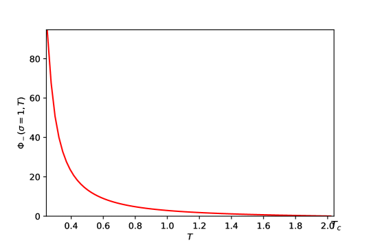
Figure 10: Plot of the rate function $\Phi_{-}(\sigma,T)$ defined by Eq. (157) as a function of $T$, for $\sigma=1$.

Behavior of the rate function $\Psi_{\sigma,T}$ near the edge: In this paragraph, we want to characterize the behavior of the function $\Psi_{\sigma,T}(w)$ near the edge $b_{-}(T)$, to see if one recovers the ‘$3/2$’ scaling as in Eq. (34) so that it matches with the asymptotic behavior of the Tracy-Widom function given in Eq. (30). Let’s consider $w=b_{-}(T)-\epsilon$, with $\epsilon>0$ and $\epsilon<<1$. Looking at small $\epsilon$ directly from Eq. (156) is difficult, since one does not have an explicit expression for $\rho_{T}(b)$. It is always possible to integrate by part and do the change of variable $b_{\pm}(\rho)=b$ in Eq. (156) to make the integrals depend only on the parametric solution $b_{\pm}(\rho)$, for which one has an explicit solution (109). However, this will give an involved expression, and it is hard to get the asymptotic at small $\epsilon$ from it. Instead, the idea is to write the large deviation function as an integral of length $\epsilon$ so that at first order in $\epsilon$ we can discretize it with Euler’s method. Let’s first notice the following integral representation for the rate function,

$$\Psi_{\sigma,T}(w) =-\int_{w}^{b_{-}(T)}(\Psi_{\sigma,T})^{\prime}(s)\,\mathrm{d}s\,,$$ (160)

where the constant of integration is zero since $\Psi_{\sigma,T}(b_{-}(T))=0$. From Eq. (154), the derivative of the rate function can be written as:

$$(\Psi_{\sigma,T})^{\prime}(s) =\frac{\mathrm{d}}{\mathrm{d}s}\left[\frac{(s-b^{\star})^{2}}{2T}-\int_{b_{-}(T)}^{b_{+}(T)}\ln(b-s)\rho_{T}(b)\mathrm{d}b-\int_{b_{-}(T)}^{b_{+}(T)}\ln\sinh\left(\frac{\sigma}{2T}(b-s)\right)\rho_{T}(b)\mathrm{d}b\right]\,,$$ (161)

$$(\Psi_{\sigma,T})^{\prime}(s) =\frac{\mathrm{d}}{\mathrm{d}s}\left[\frac{(s-b^{\star})^{2}}{2T}-\int_{b_{-}(T)}^{b_{+}(T)}\ln(b-s)\rho_{T}(b)\mathrm{d}b-\int_{b_{-}(T)}^{b_{+}(T)}\ln\left(\mathrm{e}^{\frac{\sigma}{T}b}-\mathrm{e}^{\frac{\sigma}{T}s}\right)\rho_{T}(b)\mathrm{d}b+\frac{\sigma}{T}s\right]\,,$$ (162)

where to go from Eq. (161) to Eq. (162), we have used once again the trigonometric identity (131) and discarded terms which do not depend on the variable $s$. Since $b^{\star}=1+\frac{\sigma}{2}$, this can be equivalently written as:

$$(\Psi_{\sigma,T})^{\prime}(s) =\frac{\mathrm{d}}{\mathrm{d}s}\left[\frac{(s-1)^{2}}{2T}-\int_{b_{-}(T)}^{b_{+}(T)}\ln(b-s)\rho_{T}(b)\mathrm{d}b-\int_{b_{-}(T)}^{b_{+}(T)}\ln\left(\mathrm{e}^{\frac{\sigma}{T}b}-\mathrm{e}^{\frac{\sigma}{T}s}\right)\rho_{T}(b)\mathrm{d}b\right]\,,$$ (163)

$$(\Psi_{\sigma,T})^{\prime}(s) =\frac{1}{T}(s-1)-g(s,T)-\frac{\sigma}{T}\mathrm{e}^{\frac{\sigma}{T}s}\int_{b_{-}(T)}^{b_{+}(T)}\frac{\rho_{T}(b)\mathrm{d}b}{\mathrm{e}^{\frac{\sigma}{T}s}-\mathrm{e}^{\frac{\sigma}{T}b}}\,.$$ (164)

To simplify the last term in Eq. (164), let’s introduce the matrix $\mathbf{C}=\mathrm{exp}\left\{\frac{\sigma}{T}\mathbf{B}\right\}$. The average density of the eigenvalues $\{c_{i}\}$ of the matrix $\mathbf{C}$

$$\nu(c,N) =\frac{1}{N}\,\left\langle\sum_{i=1}^{N}\delta(c_{i}-c)\right\rangle\,,$$ (165)

is related, in the large $N$ limit, to the spectral density $\rho_{T}$ by:

$$\nu(c) =\nu(c,N\to\infty)=\frac{T}{\sigma}\frac{\rho_{T}\left(\frac{T}{\sigma}\ln c\right)}{c}\,.$$ (166)

Similarly, the edges $c_{\pm}$ of the density $\nu(c)$ are given in terms of the edges $b_{\pm}(T)$ of the matrix $\mathbf{B}$ by:

$$c_{\pm} =e^{\frac{\sigma}{T}b_{\pm}(T)}\,.$$ (167)

If we introduce the resolvent $g_{C}$ of the matrix $\mathbf{C}$:

$$g_{C}(s) =\int_{\mathrm{c}_{-}}^{\mathrm{c}_{+}}\frac{\nu(c)\mathrm{d}c}{s-c}\,,$$ (168)

one can rewrite Eq. (164) as:

$$(\Psi_{\sigma,T})^{\prime}(s) =\frac{(s-1)}{T}-g(s,T)-\frac{\sigma}{T}\mathrm{e}^{\frac{\sigma}{T}s}g_{C}(\mathrm{e}^{\frac{\sigma}{T}s})\,.$$ (169)

Using the integral representation Eq. (160) for $w=b_{-}(T)-\epsilon$ together with Eq. (169), we can write the large deviation as:

$$\Psi_{\sigma,T}(b_{-}(T)-\epsilon) =-\int_{b_{-}(T)-\epsilon}^{b_{-}(T)}\left(\frac{(s-1)}{T}-g(s,T)-\frac{\sigma}{T}\mathrm{e}^{\frac{\sigma}{T}s}g_{C}(\mathrm{e}^{\frac{\sigma}{T}s})\right)\mathrm{d}s\,.$$ (170)

We can now approximate the integral by Euler’s methods:

$$\Psi_{\sigma,T}(b_{-}(T)-\epsilon) \underset{\epsilon\to 0^{+}}{\sim}\epsilon\,\times\left(\frac{(1-b_{-}(T)+\epsilon)}{T}+g(b_{-}(T)-\epsilon,T)+\frac{\sigma}{T}\mathrm{e}^{\frac{\sigma}{T}(b_{-}(T)-\epsilon)}g_{C}(\mathrm{e}^{\frac{\sigma}{T}(b_{-}(T)-\epsilon)})\right)+O(\epsilon^{2})\,.$$ (171)

Next, we need the behavior of the resolvents close to the edges:

• since the edge $b_{-}(T)$ is solution of Eq. (55), the inverse function $z(\mathrm{g})$ is locally quadratic around the point $g(b_{-}(T))$, see Fig. 6:

  $$z(\mathrm{g}) \sim b_{-}(T)+C\mathrm{g}^{2}\quad\mbox{ for }\mathrm{g}\to g(b_{-}(T))\,,$$ (172)

  where $C$ is a constant. Inverting this relation, the resolvent behaves as a square root near the edge:

  $$g(b_{-}(T)-\epsilon,T) \sim g(b_{-}(T),T)+\alpha_{B}\sqrt{\epsilon}\quad\mbox{ for }\epsilon\to 0^{+}\,,$$ (173)

  where $\alpha_{B}$ is a constant of proportionality.

• Similarly, since $c_{-}=\mathrm{e}^{\frac{\sigma}{T}b_{-}(T)}$ is the edge of the distribution $\nu(c)$ so we have:

  $$g_{C}\left(\mathrm{e}^{\frac{\sigma}{T}(b_{-}(T)-\epsilon)}\right) \sim g_{C}(c_{-})+\alpha_{C}\sqrt{\epsilon}\quad\mbox{ for }\epsilon\to 0^{+}\,,$$ (174)

  where $\alpha_{C}$ is a constant of proportionality.

This gives for the large deviation function:

$$\Psi_{\sigma,T}(b_{-}(T)-\epsilon) \sim\left(\frac{(1-b_{-}(T))}{T}+g(b_{-}(T),T)+\frac{\sigma}{T}c_{-}g_{C}\left(c_{-}\right)\right)\epsilon+\alpha\epsilon^{\frac{3}{2}}+O(\epsilon^{2})\quad\mbox{ for }\epsilon\to 0^{+}\,,$$ (175)

but using once again the trigonometric relation (131) together with the expression for the bottom edge Eq. (167), the linear term can be expressed as:

$$\frac{(1-b_{-}(T))}{T}+g(b_{-}(T),T)+\frac{\sigma}{T}c_{-}g_{C}\left(c_{-}\right) =\frac{(b^{\star}-b_{-}(T))}{T}+\int\frac{\rho_{T}(b)}{b_{-}(T)-b}\mathrm{d}b+\frac{\sigma}{2T}\int\rho_{T}(b)\coth\left(b_{-}(T)-b\right)\mathrm{d}b\,.$$ (176)

This exactly the solution of the saddle-point equation (135) for the edge $b_{-}(T)$. As a consequence, this term is exactly zero. Thus, we get the correct ‘$3/2$’ scaling, as expected:

$$\Psi_{\sigma,T}(b_{-}(T)-\epsilon) \propto\epsilon^{\frac{3}{2}}\quad\mbox{ for }\epsilon\to 0^{+}\,.$$ (177)

6 Conclusion

In this paper, we have studied the probability of stability of a large complex system of size $N$ within the framework of a generalized May model, which takes into account a possible heterogeneity $a_{i}\neq a_{j}$ in the intrinsic relaxation rates of each species. In this model, the control parameter is $T$ which is the square of the interaction strength of the random pairwise interaction between the different species. For generic distribution $\mu(a)$ of the $a_{i}$’s, Eq. (67) completely characterizes the critical point $T_{c}$ of the May-Wigner phase transition, where the system undergoes a transition from a ‘stable’ phase to an ‘unstable’ phase as $T$ increases. Focusing on the special case where the $a_{i}$’s follow what we call the flat initial condition (44), where $\sigma$ is the only new parameter of the model controlling the spread of the distribution $\mu(a)$, we are able to (i) characterize how $T_{c}$ behaves with $\sigma$, (ii) to obtain the parametric solution of the eigenvalue density of stability matrix in the large $N$ limit for any $T$, and (iii) to obtain the ‘left’ large deviation function $\Phi_{-}(\sigma,T)$ that controls the probability of stability for $T<T_{c}$ on the stable side, for large but finite $N$. One important challenge is to develop a framework to compute the ‘right’ large deviation function $\Phi_{+}(\sigma,T)$ which characterizes the probability of stability in the unstable phase $(T>T_{c})$. To compute $\Phi_{+}$, one needs to find the equilibrium measure of a pushed-to-the-origin gas of particles with a mixture of logarithmic and log-sinh pairwise interactions, as given in the joint law of eigenvalues. This remains out of reach. Finally, another natural question is to investigate the large deviation function for other initial conditions, for which we do not have a simple formula for the joint law of eigenvalues.

Appendix A Properties of the resolvent

In this section, we recall the main properties of the resolvent.

A.1 definition

For a probability distribution $\rho$, its resolvent - also known as the Green function or Stieltjes transform - is defined as:

$$g_{\rho}(z) =\int\frac{\rho(x)}{z-x}\mathrm{d}x\,.$$ (178)

The resolvent is defined for every $z$ in the complex plane except for values $z=x$ on the real line such that $\rho(x)>0$, otherwise the integral diverges.

• In particular, if $\rho$ is a smooth density function supported on an interval $[x_{-},x_{+}]$, where $x_{\pm}$ is the top/bottom edge, then its resolvent is defined for all $z\in\mathbb{C}\setminus[x_{-},x_{+}]$

  $$g_{\rho}(z) =\int_{x_{-}}^{x_{+}}\frac{\rho(x)}{z-x}\mathrm{d}x\,.$$ (179)

• Another particular case is the case where $\rho$ is a discrete measure of the form $\rho(x)=\frac{1}{N}\sum_{i=1}^{N}\delta(x-x_{i})$ which appear naturally in the context of random matrices with $\bm{x}=(x_{1},\dots,x_{N})$ the vector of eigenvalues of a matrix. In this case, the resolvent is defined for all $z\in\mathbb{C}\setminus\left\{\bm{x}\right\}$ and be simply written as:

  $$g_{\rho}(z) =\frac{1}{N}\sum_{i=1}^{N}\frac{1}{z-x_{i}}\,.$$ (180)

Resolvent of the semi-circular law: The Wigner semi-circular probability density with variance one is the average density of eigenvalues of GOE matrices as $N\to\infty$. For all $x$ in $[-2,2]$, this density is given by:

$$\rho_{\mathrm{Wig}}(x) =\frac{1}{2\pi}\sqrt{4-x^{2}}\,.$$ (181)

From Eq. (178) and integrating, one gets for the resolvent if the Wigner semi-circular distribution:

$$g_{\mathrm{Wig}}(z) =\frac{1}{2}\left(z-z\sqrt{1-\frac{4}{z^{2}}}\right)\,.$$ (182)

A.2 Inversion formula

From a resolvent, one can get back the distribution by looking at the imaginary part of the resolvent close to the support of the distribution. We have:

$$\mathfrak{Im}g(x-\mathrm{i}\epsilon) =\int\rho(x^{\prime})\mathfrak{Im}\frac{1}{x-\mathrm{i}\epsilon-x^{\prime}}\mathrm{d}x^{\prime}\,.$$ (183)

Multiplying the fraction by the conjugate of the denominator and taking only the imaginary part, one gets:

$$\mathfrak{Im}g(x-\mathrm{i}\epsilon) =\pi\left(\rho\ast P_{\epsilon}\right)(x)\,.$$ (184)

The symbol $\ast$ denotes the classical convolution product : $(f\ast g)(x)=\int f(x^{\prime})g(x-x^{\prime})\mathrm{d}x^{\prime}$ and $P_{\epsilon}$ is the Cauchy kernel defined by

$$P_{\epsilon}(x) =\frac{1}{\pi}\frac{\epsilon}{x^{2}+\epsilon^{2}}\,.$$ (185)

The kernel $P_{\epsilon}$ is the probability density of a centered Cauchy random variable with width $\epsilon$. As the width $\epsilon\to 0^{+}$, we have

$$P_{\epsilon}(x) \underset{\epsilon\to 0^{+}}{\to}\delta(x)\,,$$ (186)

where $\delta$ is a Dirac mass function. Thus, if one combines Eq. (184) and Eq. (186), one gets the Socochi-Plemelj inversion formula:

$$\rho(x) =\frac{1}{\pi}\mathfrak{Im}\,g(x-\mathrm{i}0^{+})\,.$$ (187)

A.3 edges and resolvent

Let’s consider that one has an unknown smooth density probability $\rho$, and the goal is to compute the edges $x_{\pm}$ of this density from the knowledge of the resolvent. Fix $z$ on the real line outside the support $[x_{-},x_{+}]$ where the resolvent is ill-defined. Let’s first notice that if we derive Eq. (179) with respect to $z\in\mathbb{R}$, we get:

$$g^{\prime}(z) =-\int_{x_{-}}^{x_{+}}\frac{\rho(x)}{(z-x)^{2}}<0\,,$$ (188)

and therefore the resolvent is strictly decreasing in each region $(-\infty,x_{-})$ and $(x_{+},\infty)$, and from Eq. (179). Furthermore, we have $\lim_{|z|\to\infty}g(z)=0$. Since it is decreasing on each interval, for a fixed value $\mathrm{g}$, we can always find an inverse function $z(\mathrm{g})$, also decreasing, such that $g(z(\mathrm{g}))=\mathrm{g}$. Inverse resolvent of the semi-circular law: as a concrete example, let’s look at the semi-circular distribution whose resolvent is given in Eq. (182). For $z$ real and outside the support $[x_{-},x_{+}]$, finding the inverse function $z(\mathrm{g})$ corresponds to invert the relation (182) and one gets:

$$z(\mathrm{g}) =\mathrm{g}+\frac{1}{\mathrm{g}}\,.$$ (189)

The function $z(\mathrm{g})$ is theoretically only defined between the two values $\mathrm{g}_{*}$ and $\mathrm{g}^{*}$ such that $z(\mathrm{g}_{*})=x_{-}$ and $z(\mathrm{g}^{*})=x_{+}$. Now, it turns out that one can generally extend this function $z(\mathrm{g})$ for values outside this region. The inverse resolvent of the semi-circular law is a clear example of such a case, since Eq. (189) makes sense for any $\mathrm{g}\neq 0$. However, just after the point $\mathrm{g}^{*}$ (or $\mathrm{g}_{*}$), $z(\mathrm{g})$ can not continue to be monotonic: otherwise one can invert it again to get back the resolvent $g(z)$ which would be a real function in the support of the probability distribution. This in contradiction with the Socochi-Plemelj formula (187), see Fig. 11. Hence, the derivative of the function $z(\mathrm{g})$ must cancel at the point $\mathrm{g}^{*}$ (resp. $\mathrm{g}_{*}$). Since this is the point where it takes the value $x_{+}$ (resp. $x_{-}$), we have the following properties for the edges:

$$x_{-}=z(\mathrm{g}_{*})\quad \text{and}\quad x_{+}=z(\mathrm{g}^{*})\,,$$ (190)

where $\mathrm{g}_{*}$ and $\mathrm{g}^{*}$ are respectively the lowest and highest solution of:

$$z^{\prime}(\mathrm{g}) =0\,.$$ (191)

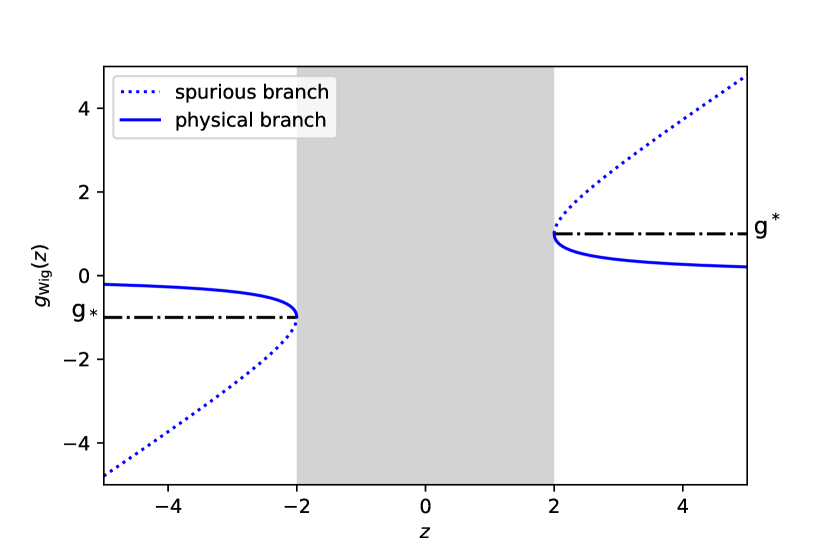
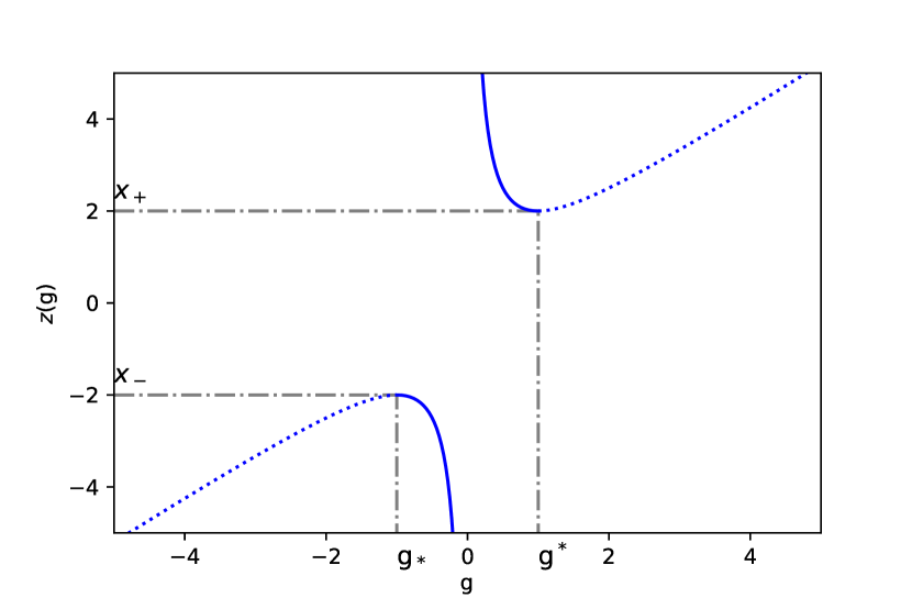
Figure 11: (Left) Plot of the resolvent for the semi-circular distribution for different value of $z$. The gray rectangle represents the region where the resolvent is not defined on the real line. The solid-line curve is the correct representation of the resolvent as given in Eq. (182) while the dotted line is the non-physical branch obtained by inverting the function $z(\mathrm{g})=\mathrm{g}+\frac{1}{\mathrm{g}}$ for values of $\mathrm{g}$ outside $[-1,1]$. (Right) Plot of the inverse function $z(\mathrm{g})=\mathrm{g}+\frac{1}{\mathrm{g}}$ of the resolvent of the semi-circular distribution. The dotted-line curve represents the analytical extension of the function outside the interval $[-1,1]$.

Recovering the edges of the semi-circular distribution: Using Eq. (191) in the case of the semi-circular distribution where the inverse resolvent is given in Eq. (189), one gets $\mathrm{g}^{*}=1=-\mathrm{g}_{*}$ and hence by Eq. (190), the edges are $x_{\pm}=\pm 2$, as expected.

References

- [1] R. M. May, “Will a large complex system be stable?,” Nature, vol. 238, no. 5364, pp. 413–414, 1972.
- [2] S. Allesina and S. Tang, “The stability–complexity relationship at age 40: a random matrix perspective,” Population Ecology, vol. 57, no. 1, pp. 63–75, 2015.
- [3] J. Moran and J.-P. Bouchaud, “May’s instability in large economies,” Physical Review E, vol. 100, no. 3, p. 032307, 2019.
- [4] H. Sompolinsky, A. Crisanti, and H.-J. Sommers, “Chaos in random neural networks,” Physical review letters, vol. 61, no. 3, p. 259, 1988.
- [5] G. Wainrib and J. Touboul, “Topological and dynamical complexity of random neural networks,” Physical review letters, vol. 110, no. 11, p. 118101, 2013.
- [6] Y. Guo and A. Amir, “Stability of gene regulatory networks,” 2020. arXiv preprint arXiv:2006.00018.
- [7] A. Amir, N. Hatano, and D. R. Nelson, “Non-Hermitian localization in biological networks,” Physical review. E, vol. 93, p. 042310, April 2016.
- [8] Y. V. Fyodorov and B. A. Khoruzhenko, “Nonlinear analogue of the May–Wigner instability transition,” Proceedings of the National Academy of Sciences, vol. 113, no. 25, pp. 6827–6832, 2016.
- [9] G. Biroli, G. Bunin, and C. Cammarota, “Marginally stable equilibria in critical ecosystems,” New Journal of Physics, vol. 20, no. 8, p. 083051, 2018.
- [10] G. Ben Arous, Y. V. Fyodorov, and B. A. Khoruzhenko, “Counting equilibria of large complex systems by instability index,” Proceedings of the National Academy of Sciences, vol. 118, no. 34, 2021.
- [11] M. L. Mehta, Random matrices. Elsevier, 2004.
- [12] P. J. Forrester, Log-gases and random matrices. Princeton University Press, 2010.
- [13] S. N. Majumdar and G. Schehr, “Top eigenvalue of a random matrix: large deviations and third order phase transition,” Journal of Statistical Mechanics: Theory and Experiment, vol. 2014, no. 1, p. P01012, 2014.
- [14] A. Krajenbrink, P. Le Doussal, and N. O’Connell, “Tilted elastic lines with columnar and point disorder, non-Hermitian quantum mechanics, and spiked random matrices: Pinning and localization,” Physical Review E, vol. 103, no. 4, p. 042120, 2021.
- [15] M. Mariño, “Chern–Simons theory, matrix integrals, and perturbative three-manifold invariants,” Communications in Mathematical Physics, vol. 253, no. 1, pp. 25–49, 2005.
- [16] M. Mariño, “Matrix models and topological strings,” in Applications of random matrices in physics, pp. 319–378, Springer, 2006.
- [17] Y. Dolivet and M. Tierz, “Chern–Simons matrix models and Stieltjes–Wigert polynomials,” Journal of mathematical physics, vol. 48, no. 2, p. 023507, 2007.
- [18] M. Tierz, “Schur polynomials and biorthogonal random matrix ensembles,” Journal of mathematical physics, vol. 51, no. 6, p. 063509, 2010.
- [19] R. J. Szabo and M. Tierz, “Chern–Simons matrix models, two-dimensional Yang–Mills theory and the Sutherland model,” Journal of Physics A: Mathematical and Theoretical, vol. 43, no. 26, p. 265401, 2010.
- [20] P. J. Forrester, “Global and local scaling limits for the = 2 Stieltjes–Wigert random matrix ensemble,” Random Matrices: Theory and Applications, p. 2250020, 2021.
- [21] E. P. Wigner, “On the statistical distribution of the widths and spacings of nuclear resonance levels,” Mathematical Proceedings of the Cambridge Philosophical Society, vol. 47, no. 4, p. 790–798, 1951.
- [22] C. A. Tracy and H. Widom, “Nonintersecting Brownian excursions,” The Annals of Applied Probability, vol. 17, no. 3, pp. 953–979, 2007.
- [23] C. A. Tracy and H. Widom, “On orthogonal and symplectic matrix ensembles,” Communications in Mathematical Physics, vol. 177, no. 3, pp. 727–754, 1996.
- [24] D. S. Dean and S. N. Majumdar, “Large deviations of extreme eigenvalues of random matrices,” Phys. Rev. Lett., vol. 97, p. 160201, 10 2006.
- [25] D. S. Dean and S. N. Majumdar, “Extreme value statistics of eigenvalues of Gaussian random matrices,” Physical Review E, vol. 77, no. 4, p. 041108, 2008.
- [26] S. N. Majumdar and M. Vergassola, “Large deviations of the maximum eigenvalue for Wishart and Gaussian random matrices,” Physical review letters, vol. 102, no. 6, p. 060601, 2009.
- [27] D. J. Gross and E. Witten, “Possible third-order phase transition in the large–N lattice gauge theory,” Physical Review D, vol. 21, no. 2, p. 446, 1980.
- [28] S. R. Wadia, “N = phase transition in a class of exactly soluble model lattice gauge theories,” Physics Letters B, vol. 93, no. 4, pp. 403–410, 1980.
- [29] P. J. Forrester, S. N. Majumdar, and G. Schehr, “Non-intersecting Brownian walkers and Yang–Mills theory on the sphere,” Nuclear Physics B, vol. 844, no. 3, pp. 500–526, 2011.
- [30] F. J. Dyson, “A Brownian-motion model for the eigenvalues of a random matrix,” Journal of Mathematical Physics, vol. 3, no. 6, pp. 1191–1198, 1962.
- [31] S. Karlin, J. McGregor, et al., “Coincidence probabilities.,” Pacific Journal of Mathematics, vol. 9, no. 4, pp. 1141–1164, 1959.
- [32] D. J. Grabiner, “Brownian motion in a Weyl chamber, non-colliding particles, and random matrices,” Annales de l’Institut Henri Poincare (B) Probability and Statistics, vol. 35, no. 2, pp. 177–204, 1999.
- [33] J. Rambeau and G. Schehr, “Distribution of the time at which vicious walkers reach their maximal height,” Phys. Rev. E, vol. 83, p. 061146, 6 2011.
- [34] J. Grela, S. N. Majumdar, and G. Schehr, “Non-intersecting Brownian bridges in the flat-to-flat geometry,” Journal of Statistical Physics, vol. 183, no. 3, pp. 1–35, 2021.
- [35] G. Menon, “Lesser known miracles of Burgers equation,” Acta Mathematica Scientia, vol. 32, no. 1, pp. 281–294, 2012.
- [36] J.-P. Blaizot and M. A. Nowak, “Universal shocks in random matrix theory,” Physical Review E, vol. 82, no. 5, p. 051115, 2010.
- [37] N. O’Connell and M. Yor, “Brownian analogues of Burke’s theorem,” Stochastic Processes and their Applications, vol. 96, no. 2, pp. 285–304, 2001.
- [38] Y. Baryshnikov, “GUEs and queues,” Probability Theory and Related Fields, vol. 119, no. 2, pp. 256–274, 2001.
- [39] C. Noack and P. Sosoe, “Concentration for integrable directed polymer models,” 2020.
- [40] Harish-Chandra, “Invariant differential operators on a semisimple Lie algebra,” Proc. Natl. Acad. Sci. USA, vol. 42, pp. 252–253, 1956.
- [41] Harish-Chandra, “Differential operators on a semisimple Lie algebra,” American Journal of Mathematics, pp. 87–120, 1957.
- [42] C. Itzykson and J.-B. Zuber, “The planar approximation. II,” Journal of Mathematical Physics, vol. 21, no. 3, pp. 411–421, 1980.
- [43] E. Brézin and S. Hikami, Random matrix theory with an external source. Springer, 2016.
- [44] E. Brézin and S. Hikami, “Level spacing of random matrices in an external source,” Physical Review E, vol. 58, no. 6, p. 7176, 1998.
- [45] P. Bleher and A. B. Kuijlaars, “Large N limit of Gaussian random matrices with external source, part I,” Communications in mathematical physics, vol. 252, no. 1, pp. 43–76, 2004.
- [46] A. I. Aptekarev, P. M. Bleher, and A. B. Kuijlaars, “Large N limit of Gaussian random matrices with external source, part II,” Communications in mathematical physics, vol. 259, no. 2, pp. 367–389, 2005.
- [47] P. M. Bleher and A. B. Kuijlaars, “Large N limit of Gaussian random matrices with external source, part III: double scaling limit,” Communications in mathematical physics, vol. 270, no. 2, pp. 481–517, 2007.
- [48] T. Claeys and D. Wang, “Random matrices with equispaced external source,” Communications in Mathematical Physics, vol. 328, no. 3, pp. 1023–1077, 2014.
- [49] K. A. Muttalib, “Random matrix models with additional interactions,” Journal of Physics A: Mathematical and General, vol. 28, no. 5, p. L159, 1995.
- [50] A. Borodin, “Biorthogonal ensembles,” Nuclear Physics B, vol. 536, no. 3, pp. 704–732, 1998.
- [51] J. Zhang, M. Kieburg, and P. J. Forrester, “Harmonic analysis for rank-1 randomised Horn problems,” 2019. arXiv preprint arXiv:1911.11316.
- [52] C. W. J. Beenakker, “Random-matrix theory of quantum transport,” Rev. Mod. Phys., vol. 69, pp. 731–808, 7 1997.
- [53] J. R. Ipsen and H. Schomerus, “Isotropic Brownian motions over complex fields as a solvable model for May–Wigner stability analysis,” Journal of Physics A: Mathematical and Theoretical, vol. 49, no. 38, p. 385201, 2016.
- [54] Y. Takahashi and M. Katori, “Noncolliding Brownian motion with drift and time-dependent Stieltjes–Wigert determinantal point process,” Journal of mathematical physics, vol. 53, no. 10, p. 103305, 2012.
- [55] A. Lenard, “Exact statistical mechanics of a one-dimensional system with Coulomb forces,” Journal of Mathematical Physics, vol. 2, no. 5, pp. 682–693, 1961.
- [56] S. Prager, “The one-dimensional plasma,” Advances in chemical physics, vol. 4, pp. 201–224, 1962.
- [57] R. J. Baxter, “Statistical mechanics of a one-dimensional coulomb system with a uniform charge background,” Mathematical Proceedings of the Cambridge Philosophical Society, vol. 59, no. 4, p. 779–787, 1963.
- [58] A. Dhar, A. Kundu, S. N. Majumdar, S. Sabhapandit, and G. Schehr, “Exact extremal statistics in the classical 1d Coulomb gas,” Physical review letters, vol. 119, no. 6, p. 060601, 2017.
- [59] A. Dhar, A. Kundu, S. N. Majumdar, S. Sabhapandit, and G. Schehr, “Extreme statistics and index distribution in the classical 1d Coulomb gas,” Journal of Physics A: Mathematical and Theoretical, vol. 51, no. 29, p. 295001, 2018.
- [60] A. Flack, S. N. Majumdar, and G. Schehr, “Truncated linear statistics in the one dimensional one-component plasma,” 2021. To appear in Journal of Physics A: Mathematical and Theoretical, arXiv:2107.14433.
- [61] J. O. Lee and K. Schnelli, “Edge universality for deformed Wigner matrices,” Reviews in Mathematical Physics, vol. 27, no. 08, p. 1550018, 2015.
- [62] A. Matytsin, “On the large-N limit of the Itzykson-Zuber integral,” Nuclear Physics B, vol. 411, no. 2-3, pp. 805–820, 1994.
- [63] J. Bun, J.-P. Bouchaud, S. N. Majumdar, and M. Potters, “Instanton approach to large N Harish-Chandra-Itzykson-Zuber integrals,” Physical review letters, vol. 113, no. 7, p. 070201, 2014.
- [64] A. Guionnet and O. Zeitouni, “Large deviations asymptotics for spherical integrals,” Journal of Functional Analysis, vol. 188, no. 2, pp. 461–515, 2002.
- [65] J.-B. Zuber, “The large-N limit of matrix integrals over the orthogonal group,” Journal of Physics A: Mathematical and Theoretical, vol. 41, no. 38, p. 382001, 2008.