One-dimensional Monte Carlo dynamics at zero temperature

Abstract

We investigate, both analytically and with numerical simulations, a Monte Carlo dynamics at zero temperature, where a random walker evolving in continuous space and discrete time seeks to minimize its potential energy, by decreasing this quantity at each jump. The resulting dynamics is universal in the sense that it does not depend on the underlying potential energy landscape, as long as it admits a unique minimum; furthermore, the long time regime does not depend on the details of the jump distribution, but only on its behaviour for small jumps. We work out the scaling properties of this dynamics, as embodied by the walker probability density. Our analytical predictions are in excellent agreement with direct Monte Carlo simulations.

I Introduction

The steepest descent method is one of the oldest optimization schemes. Cauchy, with a rather minimal mention in one of his papers, is credited for its formulation Cauchy (1847). It amounts to searching for the minimum of a well behaved function by following the steepest gradient “downhill”. A stochastic reformulation has been proposed Robbins and Monro (1951), to alleviate the computational cost of working in spaces with large dimensions: the gradient is then estimated over a restricted set of directions, drawn randomly Spall (2012). This technique is widely used in machine learning Sra et al. (2011).

We are interested here in a minimal version of stochastic gradient descent, in a one-dimensional setting. A random walker on the line, with position denoted by $x$, moves by random jumps; the move is accepted only if it leads to the decrease of some objective function $U(x)$, referred to as the potential. In this respect, the walker is greedy, performing moves that always decrease $U$. We assume that $U$ admits a single minimum: we are not interested in finding this point (taken as $x=0$ below), but rather in the dynamics of the walker upon approaching it. The specific form of the potential is immaterial; it does not need to be symmmetric, as long as it has no local minima, beyond the global maximum at $x=0$. Such an algorithm can be viewed as the vanishing temperature limit of a standard Metropolis sampling, a Monte-Carlo method where a Markov chain is constructed to sample the phase space according to a predefined target distribution Frenkel and Smith (2002); Newman and Barkema (1999); Krauth (2006). As simple as it is –the walker position distribution function is increasingly peaked at $x=0$– such a dynamics exhibits non trivial features, depending on the sampling chosen. A key role is indeed played by the probability distribution of attempted jumps, and in particular, its behaviour for small jumps. The present $T=0$ problem differs from widespread approaches such as simulated annealing, where the temperature ruling the evolution of a random walker is gradually decreased, in order to find minima in a given potential landscape. Here, the motivation is different: the location of the potential minimum is known, and we are interested in the dynamics towards this target.

Starting from the Metropolis rule, we define in section II the dynamics, in discrete time $n=0,1,\ldots$. The walker’s density $P_{n}(x)$ evolves at long time towards $P_{\infty}(x)=\delta(x)$, where $\delta$ denotes the Dirac distribution. Our goal is to resolve the approach to this limiting form, that takes place in a self-similar way. We show indeed in section III that $P_{n}(x)$ admits a scaling form at long times, where the whole position and temporal information is encoded in a single universal scaling function, independent of $U(x)$ and the initial condition. Its generic properties are studied analytically. A number of exact solutions, presented in section IV corroborate the general findings, and provide additional insights into the long time dynamics. All predictions fare well compared to Monte Carlo simulations, where the original dynamics is directly implemented.

II The Model

We consider a single particle moving on a line in the presence of an external confining potential $U(x)$, having a single minimum, and no local minima. In other words, $U(x)$ should be a monotonically increasing function of $|x|$. At time $n$, an attempted jump $\eta_{n}$ is drawn from a distribution $w(\eta)$ and the particle moves according to the Metropolis rules

$$x_{n}=\begin{cases}x_{n-1}+\eta_{n}&{\rm with}\,\,{\rm prob.}\,\,\,p={\rm min}\left(1,e^{-\beta\,\Delta U}\right)\quad{\rm where}\quad\Delta U=U(x_{n-1}+\eta_{n})-U(x_{n-1})\\ \\ x_{n-1}&{\rm with}\,\,{\rm prob.}\,\,\,1-p\,,\end{cases}$$ (1)

where $\beta$ is for inverse temperature $(k_{B}T)^{-1}$. The position distribution $P_{n}(x)$ evolves via the Master equation

$$P_{n}(x)=\int_{-\infty}^{\infty}dx^{\prime}\,P_{n-1}(x^{\prime})\,w(x-x^{\prime})\,{\rm min}\left(1,e^{-\beta\,\left(U(x)-U(x^{\prime})\right)}\right)+\left[1-\int_{-\infty}^{\infty}dx^{\prime}\,w(x^{\prime}-x)\,{\rm min}\left(1,e^{-\beta\,\left(U(x^{\prime})-U(x)\right)}\right)\right]\,P_{n-1}(x),$$ (2)

where the jump distribution $w(\eta)$ is assumed to be symmetric: $w(\eta)=w(-\eta)$. It is convenient to replace the ‘min’ function above by the following identity

$${\rm min}\left(1,e^{-\beta\,\left(U(x)-U(x^{\prime})\right)}\right)=\theta\left(U(x^{\prime})-U(x)\right)+e^{-\beta\,\left(U(x)-U(x^{\prime})\right)}\,\theta\left(U(x)-U(x^{\prime})\right)\,$$ (3)

where $\theta(z)$ is the Heaviside theta function: $\theta(z)=1$ if $z>0$ and $\theta(z)=0$ if $z<0$.

We now focus on the limit $T=0$, i.e., $\beta=\infty$ . In this limit, (3) becomes

$${\rm min}\left(1,e^{-\beta\,\left(U(x)-U(x^{\prime})\right)}\right)=\theta\left(U(x^{\prime})-U(x)\right)=\theta\left(|x^{\prime}|-|x|\right)$$ (4)

where in arriving at the last equality we used the fact that the potential increases monotonically with $|x|$ so that $U(x^{\prime})>U(x)$ implies $|x^{\prime}|>|x|$. Thus, in this limit, the particle can jump only downhill, and all uphill moves are forbidden. More precisely, if the particle is at $x$ at step $n$, then in the next step it can jump only to the region $x^{\prime}\in[-|x|,|x|]$. Any jump that takes it outside this region is forbidden at $T=0$ (see Fig. 1). Thus the explicit dependence of the position distribution $P_{n}(x)$ on the form of the potential $U(x)$ drops out in this $T=0$ limit, that can naturally be simulated by a Monte Carlo method, as described in Appendix A. However, even in this relatively simple limit, the evolution of the position distribution remains rather nontrivial. With the simplification in (4), the Master equation (2) reduces to a simpler form

$$P_{n}(x)=\int_{-\infty}^{\infty}dx^{\prime}\,P_{n-1}(x^{\prime})\,w(x-x^{\prime})\,\theta\left(|x^{\prime}|-|x|\right)+\left[1-\int_{-\infty}^{\infty}dx^{\prime}\,w(x^{\prime}-x)\,\theta\left(|x|-|x^{\prime}|\right)\right]\,P_{n-1}(x)\,.$$ (5)

One can check that Eq. (5) satisfies the probability conservation

$$\int_{-\infty}^{\infty}P_{n}(x)\,dx=\int_{-\infty}^{\infty}P_{n-1}(x)\,dx\,.$$ (6)

Since the particle moves only downhill, we expect that at long times, i.e., in the limit $n\to\infty$, the position distribution should approach a delta function at the origin (irrespective of the initial condition)

$$\lim_{n\to\infty}P_{n}(x)=\delta(x)\,.$$ (7)

We are interested in computing how the position distribution relaxes to this steady state.

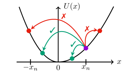
Figure 1: Possible moves of a particle at $T=0$ in the potential $U(x)$, that monotonically increases with $|x|$. Only downhill stochastic moves are allowed (greedy motion). If at step $n$, the particle is at $x_{n}$, then at the next step it can jump only into the region $[-x_{n},x_{n}]$. Any jump that takes the particle outside this interval is forbidden at $T=0$.

For the analytical work, it is convenient to start from a symmetric initial condition. This ensures that at all times $P_{n}(x)$ is also symmetric, $P_{n}(x)=P_{n}(-x)$. In that case, we can just focus on $x\geq 0$. This symmetry assumption will be tested against numerical simulations, run in conditions of asymmetric initial conditions. It will be seen that the dynamics gradually suppresses non-symmetrical features of the position distribution. An explicit solution in a specific case will confirm this computational observation. Our Master equation (5) then reads (restricted to $x\geq 0$)

$$P_{n}(x)=\int_{-\infty}^{-x}dx^{\prime}\,P_{n-1}(x^{\prime})\,w(x-x^{\prime})+\int_{x}^{\infty}dx^{\prime}\,P_{n-1}(x^{\prime})\,w(x-x^{\prime})+\left[1-\int_{-x}^{x}dx^{\prime}\,w(x^{\prime}-x)\right]\,P_{n-1}(x)\,.$$ (8)

In the first integral on the right hand side (r.h.s) we make the change of variable $x^{\prime}\to-x^{\prime}$ and use the symmetry $P_{n}(x)=P_{n}(-x)$ to get for all $x\geq 0$

$$P_{n}(x)-P_{n-1}(x)=\int_{x}^{\infty}dx^{\prime}\,P_{n-1}(x^{\prime})\,\left[w(x+x^{\prime})+w(x-x^{\prime})\right]-\left[\int_{-x}^{x}dx^{\prime}\,w(x^{\prime}-x)\right]\,P_{n-1}(x)\,.$$ (9)

III Scaling analysis of the Master equation: asymptotic results

III.1 The scaling ansatz

The integral equation (9) is still hard to solve exactly for all $n$ and for arbitrary symmetric jump distribution $w(\eta)$. However, in the large $n$ limit, further simplifications occur. Indeed, for large $n$ we make a scaling ansatz for $P_{n}(x)$ that should be verified a posteriori and also confirmed numerically. Our ansatz reads

$$P_{n}(x)=B\,n^{\alpha}\,F\left(B\,n^{\alpha}\,x\right)\,,$$ (10)

where the exponent $\alpha>0$ and the scale factor $B$ will be selected subsequently. In doing so, we seek to “resolve” the structure of the asymptotic Dirac delta distribution, towards which the position distribution evolves. Since $P_{n}(x)$ is taken here symmetric around $x=0$, the scaling function $F(z)$ is symmetric: $F(z)=F(-z)$. In addition, from the normalization of $P_{n}(x)$, the scaling function $F(z)$ must satisfy the constraint

$$\int_{-\infty}^{\infty}F(z)\,dz=1\,.$$ (11)

The scaling form in (10) makes sense physically. It stipulates that the width of the distribution decreases for large time $n$ as $\sim n^{-\alpha}$ with $\alpha>0$, while the value at the peak increases as $n^{\alpha}$. Thus, as $n$ increases, the position distribution function $P_{n}(x)$ gets more and more peaked near $x=0$, and eventually approaches the delta function $P_{n}(x)\to\delta(x)$ as $n\to\infty$.

We substitute this scaling ansatz (10) in the Master equation (9) and evaluate the left hand side (l.h.s) and the r.h.s. For large $n$, the l.h.s simplifies to

$$P_{n}(x)-P_{n-1}(x)\approx\frac{\partial P_{n}(x)}{\partial n}\approx B\,\alpha\,n^{\alpha-1}\,\left[F(z)+z\,F^{\prime}(z)\right]\,,\quad{\rm where}\quad z=B\,n^{\alpha}\,x\,.$$ (12)

We now substitute the scaling ansatz (10) on the r.h.s of (9). After making the change of variable $z^{\prime}=B\,n^{\alpha}\,x^{\prime}$ inside the integrals on the r.h.s of (9), it reads

$$\text{r.h.s}\approx\int_{z}^{\infty}dz^{\prime}\,F(z^{\prime})\,\left[w\left(\frac{z+z^{\prime}}{B\,n^{\alpha}}\right)+w\left(\frac{z-z^{\prime}}{B\,n^{\alpha}}\right)\right]-\left(\int_{-z}^{z}dz^{\prime}\,w\left(\frac{|z^{\prime}-z|}{B\,n^{\alpha}}\right)\right)\,F(z)\,.$$ (13)

Since we assumed $\alpha>0$ (to be verified a posteriori), it follows that as $n\to\infty$, the arguments of the function $w$ in (13) approach $0$. Hence, the scaling behavior depends crucially on how the jump distribution function $w(\eta)$ behaves for small $|\eta|$. We consider the following natural class of power law behaviors near $\eta=0$

$$w(\eta)\approx C_{p}\,|\eta|^{p}\quad{\rm as}\quad\eta\to 0\,,$$ (14)

where $C_{p}>0$ is a positive constant and $p>-1$ to ensure the normalization. Substituting this behavior on the r.h.s in (13) and equating it to the l.h.s in (12) we get, to leading order for large $n$,

$$B\,\alpha\,n^{\alpha-1}\,\left[F(z)+z\,F^{\prime}(z)\right]=\frac{C_{p}}{B^{p}}\,n^{-\alpha p}\,\left[\int_{z}^{\infty}dz^{\prime}\,\left[(z+z^{\prime})^{p}-(z^{\prime}-z)^{p}\right]\,F(z^{\prime})-\left(\int_{-z}^{z}dz^{\prime}\,|z^{\prime}-z|^{p}\right)\,F(z)\right]\,.$$ (15)

Note that $F^{\prime}(z)=dF(z)/dz$. In order that both sides scale as the same power of $n$ for large $n$, we must have the exponent

$$\alpha=\frac{1}{1+p}\,.$$ (16)

Furthermore, let us choose the scale factor $B$ as

$$B=\left[C_{p}(1+p)\right]^{1/{1+p}}\,.$$ (17)

With this choice of $B$, the scaling function $F(z)$ now depends only on the single parameter $p$, hence we will denote it by $F_{p}(z)$. It then satisfies the integro-differential equation in $z\geq 0$, obtained from (15)

$$F_{p}(z)+z\,F_{p}^{\prime}(z) = \int_{z}^{\infty}dz^{\prime}\,\left[(z^{\prime}+z)^{p}+(z^{\prime}-z)^{p}\right]\,F_{p}(z^{\prime})-\left(\int_{0}^{z}dz^{\prime}\,\left[(z+z^{\prime})^{p}+(z-z^{\prime})^{p}\right]\right)\,F_{p}(z)\,$$ (18)

$$= \int_{z}^{\infty}dz^{\prime}\,\left[(z^{\prime}+z)^{p}+(z^{\prime}-z)^{p}\right]\,F_{p}(z^{\prime})-\frac{(2z)^{1+p}}{1+p}\,F_{p}(z)\,.$$

To summarise, we justified a posteriori that the position distribution $P_{n}(x)$ satisfies the scaling form

$$P_{n}(x)\approx B\,n^{1/(1+p)}\,F_{p}\left(B\,n^{1/(1+p)}\,x\right)\,,\quad{\rm where}\quad B=\left[C_{p}(1+p)\right]^{1/(1+p)}\,,$$ (19)

and the scaling function $F_{p}(z)$, indexed by $p$, is determined from the solution of the integro-differential equation (18). Note that $F_{p}(z)$ is symmetric in $z$ and hence satisfies the normalization condition

$$\int_{0}^{\infty}F_{p}(z)\,dz=\frac{1}{2}\,.$$ (20)

Thus the scaling function $F_{p}(z)$ depends only on the index $p$, but otherwise is universal, i.e., independent of the details of the jump distribution $w(\eta)$. For general $p>-1$, it is hard to solve the integro-differential (18) exactly. However, as we show below, one can derive the asymptotic behaviors of $F_{p}(z)$ as $z\to\infty$ and as $z\to 0$ for general $p>-1$. Later, we show that for the three special cases, $p=0$, $p=1$ and $p=2$, it is possible to obtain exact solutions for the full scaling function $F_{p}(z)$.

III.2 Large $z$ behavior of $F_{p}(z)$

For large $z$, the l.h.s of (18) is dominated by the second term $zF_{p}^{\prime}(z)$. In contrast, for large $z$, the first term on the r.h.s of (18) goes to zero, while the second term dominates, as can be checked a posteriori. Hence, for large $z$, we get $z\,F_{p}^{\prime}(z)\approx-[(2z)^{p+1}/(p+1)]\,F_{p}(z)$. Integrating, we obtain for large $z$ and any $p>-1$

$$F_{p}(z)\sim\exp\left[-\frac{{2}^{p+1}}{(1+p)^{2}}\,z^{1+p}\right]\,.$$ (21)

This result has a neat physical interpretation. In fact, expressing the scaled variable $z=B\,n^{1/(p+1)}x$ in terms of the original distance variable $x$, one finds (up to power law prefactors)

$$P_{n}(x)\sim F_{p}(z)\sim\exp\left[-\frac{C_{p}}{1+p}\,(2\,x)^{p+1}\,n\right]\,.$$ (22)

Hence $P_{n}(x)$ decays exponentially with increasing $n$ for fixed $x$. This can be understood from a very simple Poisson type of argument. Consider the particle to be at $x$ at large time $n$ such that $B^{-1}\,n^{-1/(1+p)}\ll|x|\ll 1$. In this regime $|z|=B\,n^{1/(1+p)}|x|\gg 1$. From this position the particle attempts a jump. It succeeds if the jump takes it into $x^{\prime}\in[-x,x]$, otherwise it is unsuccessful and the particle stays at $x$. Also, the influx of probability to $x$ from higher values of $|x|$ is negligible in this regime. Hence, the probability to stay at $x$ after step $n$ is approximately

$$P_{n}(x)\sim\left[1-p_{\rm accept}(x)\right]^{n}\,,$$ (23)

where the acceptance probability at $x$ is given by

$$p_{\rm accept}(x)=\int_{-x}^{x}dx^{\prime}w(x^{\prime}-x)=\int_{0}^{x}\left[w\left(x+x^{\prime}\right)+w\left(|x-x^{\prime}|\right)\right]\,dx^{\prime}.$$ (24)

Since $|x|\ll 1$, the argument of $w$ is small and we can expand in Taylor series. Keeping only the leading order term for $|x|\ll 1$ and using (14), we obtain

$$p_{\rm accept}(x)\approx\frac{C_{p}}{(1+p)}\,(2\,x)^{1+p}\,.$$ (25)

Substituting this result in (23), we recover, for large $n$, the result in (22).

III.3 Small $z$ behavior of $F_{p}(z)$

Extraction of the small $z$ behavior of $F_{p}(z)$ from (18) is non trivial. We consider the r.h.s of (18) and start with the small $z$ behavior of the first term $\int_{z}^{\infty}dz^{\prime}\,\left[(z^{\prime}+z)^{p}+(z^{\prime}-z)^{p}\right]\,F_{p}(z^{\prime})$. Consider the first integral and rewrite it as

$$R_{1}=\int_{z}^{\infty}dz^{\prime}\,(z^{\prime}+z)^{p}\,F_{p}(z^{\prime})=\int_{2z}^{\infty}du\,u^{p}\,F_{p}(u-z)\,.$$ (26)

We now expand $F_{p}(u-z)$ in Taylor series for small $z$ and keep terms up to $O(z^{2})$. Furthermore, we rewrite the integral $\int_{2z}^{\infty}=\int_{0}^{\infty}-\int_{0}^{2z}$ and then expand the second part also for small $z$. After some algebra, this gives for small $z$

$$R_{1}=b_{0}+b_{1}\,z+b_{2}\,z^{2}-\frac{F_{p}(0)}{1+p}\,(2z)^{p+1}+O(z^{\gamma})\,,$$ (27)

with

$$b_{k}=\frac{(-1)^{k}}{k!}\,\int_{0}^{\infty}du\,u^{p}\,F_{p}^{(k)}(u)\,,\quad{\rm where}\quad F_{p}^{(k)}(u)=\frac{dF_{p}^{k}(u)}{du^{k}}\,.$$ (28)

The exponent $\gamma$ is given by

$$\gamma=\min(3,p+2)\,.$$ (29)

Repeating the same exercise with the second integral we get

$$R_{2} = \int_{z}^{\infty}dz^{\prime}\,(z^{\prime}-z)^{p}\,F_{p}(z^{\prime})=\int_{0}^{\infty}du\,u^{p}\,F_{p}(u+z)$$ (30)

$$= b_{0}+b_{1}\,z+b_{2}\,z^{2}+O(z^{3})\,.$$

Adding (27) and (30), and substituting on the r.h.s of Eq. (18), we get

$$F_{p}(z)+z\,F_{p}^{\prime}(z)=\frac{d}{dz}[zF_{p}(z)]=2\,b_{0}+2\,b_{2}\,z^{2}-2\frac{F_{p}(0)}{1+p}\,(2z)^{p+1}+O(z^{\gamma})$$ (31)

Integrating we get for small $z$

$$F_{p}(z)=2\,b_{0}\,+\frac{2b_{2}}{3}\,z^{2}-\frac{2^{p+2}F_{p}(0)}{(1+p)(2+p)}\,z^{1+p}+O(z^{\gamma})\,.$$ (32)

Thus, while the leading term is always $2\,b_{0}$, the subleading term depends on the value of $p$. Let us distinguish between three cases.

• $p>1$: In this case, the first two terms in the small $z$ expansion of $F_{p}(z)$ are

  $$F_{p}(z)\to a_{0}+a_{2}\,z^{2}$$ (33)

  where the two coefficients are given by

  $$a_{0} = 2\,b_{0}=2\int_{0}^{\infty}du\,u^{p}\,F_{p}(u)$$ (34)

  $$a_{2} = \frac{2b_{2}}{3}=\frac{1}{3}\int_{0}^{\infty}du\,u^{p}\,F_{p}^{\prime\prime}(u)=\frac{p(p-1)}{3}\,\int_{0}^{\infty}du\,u^{p-2}\,F_{p}(u)\,.$$ (35)

  Note that since $a_{2}>0$, the function $F_{p}(z)$ for small $z$ actually increases as $z$ increases. Finally as $z\to\infty$, $F_{p}(z)$ has to decay as in (21). Hence, the function $F_{p}(z)$ is non-monotonic as a function of $z$ for $p>1$. If one considers the symmetrized version of $F_{p}(z)$, there is a local minimum (a hole) at $z=0$ (see Fig. 4 for the case $p=2$).

• $-1<p<1$: In this case, the first two terms are given by

  $$F_{p}(z)\to a_{0}+a_{p+1}\,z^{p+1}$$ (36)

  where the coefficients read

  $$a_{0} = 2\,b_{0}=2\int_{0}^{\infty}du\,u^{p}\,F_{p}(u)$$ (37)

  $$a_{p+1} = -\frac{2^{p+2}F_{p}(0)}{(1+p)(2+p)}\,.$$ (38)

  Thus in this case, since $a_{p+1}<0$, the function $F_{p}(z)$ decreases as $z$ increases from $0$, indicating that for $-1<p<1$, the scaling function $F_{p}(z)$ is likely to be a monotonically decreasing function of $z$, with a single peak at $z=0$, see Fig. 2 for $p=0$.

• $p=1$: Finally in the marginal case $p=1$, where one has to merge the second and the third term together on the r.h.s of (32), one gets

  $$F_{p}(z)\to a_{0}+a_{2}\,z^{2}$$ (39)

  where the coefficients are

  $$a_{0} = 2\,b_{0}=2\int_{0}^{\infty}du\,u\,F_{1}(u)$$ (40)

  $$a_{2} = \frac{1}{3}\,\int_{0}^{\infty}du\,u\,F_{1}^{\prime\prime}(u)-\frac{4}{3}F_{1}(0)=-F_{1}(0)\,.$$ (41)

  As we will see later, in this case we can derive the full solution exactly, $F_{1}(z)=(1/\sqrt{\pi})\,e^{-z^{2}}$ whose small $z$ expansion agrees with (40) and (41).

Let us then summarize the asymptotic behavior of $F_{p}(z)$ for general $p>-1$. Using the symmetry of $F_{p}(z)$ we get

$$F_{p}(z)\sim\exp\left[-\frac{{2}^{p+1}}{(1+p)^{2}}\,|z|^{1+p}\right]\,\quad{\rm as}\quad|z|\to\infty\,.$$ (42)

The small $z$ behavior depends on the index $p$ and the first two terms are given by

$$F_{p}(z)\to\begin{cases}2\,\int_{0}^{\infty}du\,u^{p}\,F_{p}(u)-\left[\frac{2^{p+2}\,F_{p}(0)}{(1+p)(2+p)}\right]\,|z|^{p+1}\,&{\rm for}\quad-1<p<1\\ \\ 2\,\int_{0}^{\infty}du\,u^{p}\,F_{1}(u)-\left[F_{1}(0)\right]\,z^{2}\,&{\rm for}\quad p=1\\ \\ 2\,\int_{0}^{\infty}du\,u^{p}\,F_{p}(u)+\left[\frac{p(p-1)}{3}\int_{0}^{\infty}du\,u^{p-2}\,F_{p}(u)\right]\,z^{2}\,&{\rm for}\quad p>1\,.\end{cases}$$ (43)

There is thus a change of the small $z$ behavior at $p=1$, from a decreasing function of $|z|$ for $|p|<1$ to an increasing one for $p>1$. Indeed, with a probability density of jumps $w(\eta)\propto|\eta|^{p}$, $p>1$ does penalize the occurrence of the small jumps, required to move, as compared to the case $p<1$. When $p>1$, the reduced likelihood of small jumps leads to a depletion of $F_{p}(z)$ at $z=0$. Beyond the asymptotic results derived here, we present in the next section exact solutions for the three special cases $p=0$, $p=1$ and $p=2$.

IV Exact scaling solutions

IV.1 Exact solution for $p=0$

The case $p=0$ includes most natural symmetric jump distributions such as

• Gaussian: $w(\eta)=\frac{1}{\sqrt{2\,\pi}}\,e^{-\eta^{2}/2}$

• Double-exponential: $w(\eta)=\frac{1}{2}\,e^{-|\eta|}$, see also Appendix B.

• Uniform distribution: $w(\eta)=\frac{1}{2}\,\left[\theta(\eta+1)-\theta(\eta-1)\right]$.

• Long-ranged distributions such as $w(\eta)=1/[\pi(1+\eta^{2})]$, the Cauchy jump distribution.

In all these cases, $w(\eta)\to{\rm const.}$ as $\eta\to 0$, implying $p=0$. In this case, the integro-differential equation (18) reads

$$F_{0}(z)+z\,F_{0}^{\prime}(z)=2\,\int_{z}^{\infty}dz^{\prime}F_{0}(z^{\prime})-2\,z\,F_{0}(z)\,,$$ (44)

and it must satisfy the normalization condition (20) together with the large $z$ asymptotic behavior (42). The solution of (44) turns out to be simple, as can be checked by direct substitution:

$$F_{0}(z)=e^{-2\,z}\,,\quad{\rm for}\quad z\geq 0.$$ (45)

The large and small $z$ behaviors in (42) and (43) are consistent with the exact solution (45), as can be checked easily. Thus for $p=0$, our prediction is that $P_{n}(x)$ is given by the scaling form

$$P_{n}(x)\approx C_{0}\,n\,F_{0}\left(C_{0}\,n\,x\right)\,,\quad{\rm with}\quad F_{0}(z)=e^{-2|z|}\,,$$ (46)

where we used the symmetry $F_{0}(z)=F_{0}(-z)$ and $C_{0}=w(0)$. In Fig. 2, we compare our theoretical prediction for $F_{0}(z)$ with the numerical simulations (see Appendix A for details on the numerical aspects), obtained for three different jump distributions all with $p=0$, namely the Gaussian, the double-exponential and the uniform jump distributions. We find excellent agreement between the theoretical prediction and the simulations. The slight asymmetry observed between positive and negative values of $x$ is a fingerprint of the asymmetric initial conditions. Its progressive disappearance gives an idea on the speed of convergence towards the scaling form. We come back to this question in Appendix B.

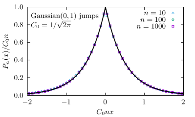
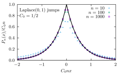
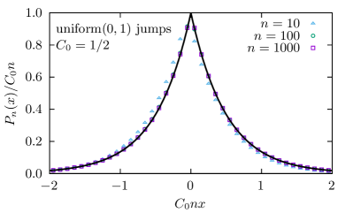
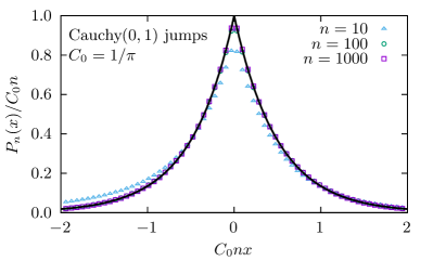
Figure 2: Case $p=0$. Scaling function $F_{0}(z)$ obtained from the simulation data and the scaled $P_{n}(x)$ as in (46), compared with the theoretical prediction of the universal form $F_{0}(z)=e^{-2|z|}$. Four different jump distributions $w$ have been used: the Gaussian, the Laplace, the uniform and the Cauchy distributions, all having $p=0$. While the measurements for small times ($n=10$) show deviations and an asymmetry due to the initial position chosen in the simulations ($x_{0}=-1$), the convergence towards the form (46) is already very good for $n=1000$ in all tested distributions. Measurements averaged over $10^{7}$ independent runs.

IV.2 Exact solution for $p=1$

An example of a jump distribution that belongs to the $p=1$ class is the symmetric Weibull distribution (normalized to unity)

$$w(\eta)=|\eta|\,e^{-\eta^{2}}\,.$$ (47)

In this case, setting $p=1$ in (18) we get

$$F_{1}(z)+z\,F_{1}^{\prime}(z)=2\,\int_{z}^{\infty}dz^{\prime}\,z^{\prime}\,F_{1}(z^{\prime})-2\,z^{2}\,F_{1}(z)\,,$$ (48)

where the solution $F_{1}(z)$ should satisfy the normalization condition $\int_{0}^{\infty}F_{1}(z)\,dz=1/2$ and also the large $z$ asymptotic behavior in (42) with $p=1$. Remarkably, (48) also admits a simple solution (as can be checked by direct verification)

$$F_{1}(z)=\frac{1}{\sqrt{\pi}}\,e^{-z^{2}}\,,$$ (49)

where the prefactor is chosen such that $\int_{0}^{\infty}F_{1}(z)\,dz=1/2$. It is immediate to check that this exact solution is compatible with the large and small $z$ behaviors in (42) and (43). Thus, for $p=1$, our scaling prediction for the position distribution $P_{n}(x)$ reads

$$P_{n}(x)\approx\sqrt{2\,C_{1}}\,n^{1/2}\,F_{1}\left(\sqrt{2\,C_{1}}\,n^{1/2}\,x\right)\,\quad{\rm with}\quad F_{1}(z)=\frac{1}{\sqrt{\pi}}\,e^{-z^{2}}\,,$$ (50)

where we again used the symmetry $F_{1}(z)=F_{1}(-z)$ and $B=\sqrt{2\,C_{1}}$ for $p=1$ from (19). In Fig. 3, we compare the theoretical prediction for $F_{1}(z)$ in (50) with the numerically obtained $F_{1}(z)$ using the symmetric Weibull jump distribution in (47), finding excellent agreement.

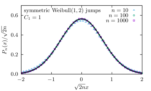
Figure 3: Case $p=1$. The scaling function $F_{1}(z)$ obtained from the simulation data for the scaled $P_{n}(x)$ as in (50), compared with the theoretical prediction of the universal form $F_{1}(z)=(1/\sqrt{\pi})\,e^{-z^{2}}$. In the simulation, we used the symmetric Weibull jump distribution with shape factor 2 shown in (47), thus $C_{1}=1$. The agreement for $n\geq 100$ is excellent. Measurements obtained from $10^{7}$ independent runs with $n=1000$ jumps each. Here again, the slight $x\to-x$ asymmetry observed at early times is a consequence of having chosen an asymmetric initial condition.

IV.3 Exact solution for $p=2$

We now consider the case $p=2$. This corresponds to symmetric jump distribution $w(\eta)$ with the small $\eta$ behavior

$$w(\eta)\to C_{2}\,\eta^{2}\quad{\rm as}\quad\eta\to 0\,.$$ (51)

Then, the scaling theory for the position distribution (19) predicts that for large $n$

$$P_{n}(x)\approx(3\,C_{2}\,n)^{1/3}\,F_{2}\left((3\,C_{2}\,n)^{1/3}\,x\right)\,,$$ (52)

where the scaling function $F_{2}(z)=F_{2}(-z)$ is symmetric and is normalized $\int_{0}^{\infty}F_{2}(z)\,dz=1/2$. The scaling function $F_{2}(z)$, setting $p=2$ in (18), satisfies the integro-differential equation (restricting only to $z\geq 0$)

$$F_{2}(z)+z\,F_{2}^{\prime}(z)=2z^{2}\int_{z}^{\infty}dz^{\prime}\,F_{2}(z^{\prime})+2\,\int_{z}^{\infty}dz^{\prime}\,(z^{\prime})^{2}\,F_{2}(z^{\prime})-\frac{8z^{2}}{3}\,F_{2}(z)\,,$$ (53)

where $F_{2}^{\prime}(z)=dF_{2}(z)/dz$. The function $F_{2}(z)$ must approach a constant as $z\to 0$ and should decay as $F_{2}(z)\sim\exp[-8z^{3}/9]$ as $z\to\infty$: this follows from the general asymptotics in (42) and (43). In addition, it must satisfy the normalization condition (20).

To solve this integro-differential equation (53), the strategy would be first to reduce it to a differential equation. To do this, let us define the cumulative scaling function

$$G_{2}(z)=\int_{z}^{\infty}F_{2}(z^{\prime})\,dz^{\prime}\,.$$ (54)

We have $G_{2}^{\prime}(z)=-F_{2}(z)$ and $G_{2}(z)\to 0$ as $z\to\infty$. Now consider the second term on the r.h.s of (53). With an integration by parts, we can rewrite it as

$$-\int_{z}^{\infty}dz^{\prime}(z^{\prime})^{2}G_{2}^{\prime}(z)=z^{2}\,G_{2}(z)+2\,\int_{z}^{\infty}z^{\prime}\,G_{2}(z^{\prime})\,dz^{\prime}\,.$$ (55)

Thus, using $F_{2}(z)=-G_{2}^{\prime}(z)$, Eq. (53) reads

$$-\left[1+\frac{8z^{3}}{3}\right]G_{2}^{\prime}(z)-z\,G_{2}^{\prime\prime}(z)-4\,z^{2}\,G_{2}(z)=4\,\int_{z}^{\infty}z^{\prime}\,G_{2}(z^{\prime})\,dz^{\prime}\,.$$ (56)

Differentiating once more with respect to $z$ gives a differential equation for $G_{2}(z)$

$$z\,G_{2}^{\prime\prime\prime}(z)+\left[2+\frac{8z^{3}}{3}\right]\,G_{2}^{\prime\prime}(z)+12z^{2}G_{2}^{\prime}(z)+4zG_{2}(z)=0\,.$$ (57)

We divide by $z$, differentiate once more with respect to $z$ and use $G_{2}^{\prime}(z)=-F_{2}(z)$ to finally obtain a third order ordinary differential equation for $F_{2}(z)$

$$F_{2}^{\prime\prime\prime}(z)+\left[\frac{2}{z}+\frac{8z^{2}}{3}\right]F_{2}^{\prime\prime}(z)+\left[-\frac{2}{z^{2}}+\frac{52z}{3}\right]\,F_{2}^{\prime}(z)+16F_{2}(z)=0\,.$$ (58)

A symbolic calculation software Inc. allows to solve this equation, and it gives the general solution as a linear combination of three independent functions

$$F_{2}(z)=(A_{1})\,{}_{1}F_{1}\left(\frac{1}{2},\frac{1}{3},-\frac{8z^{3}}{9}\right)+(A_{2})\,z^{2}\,{}_{1}F_{1}\left(\frac{7}{6},\frac{5}{3},-\frac{8z^{3}}{9}\right)+(A_{3})\,G_{2,2}^{2,2}\left(\begin{array}[]{l}-\frac{1}{3},\phantom{-}\frac{1}{2}\\ -\frac{1}{3},-\frac{2}{3}\end{array}\middle|-\frac{8z^{3}}{9}\right)\,,$$ (59)

where ${}_{1}F_{1}(a,b,z)$ is the Kummer’s confluent hypergeometric function and $G_{m,n}^{p,q}$ denotes the Meijer’s G function. The constants $A_{1}$, $A_{2}$ and $A_{2}$ have to be determined from boundray conditions. First we note that the third function $G_{m,n}^{p,q}$ diverges as $1/z$ as $z\to 0$. Since this is not allowed (the scaling function $F_{2}(z)$ is normalizable and approaches a constant as $z\to 0$ from (43)). Hence we must have $A_{3}=0$. Thus

$$F_{2}(z)=A_{1}\,\left[{}_{1}F_{1}\left(\frac{1}{2},\frac{1}{3},-\frac{8z^{3}}{9}\right)+B_{2}\,z^{2}\,{}_{1}F_{1}\left(\frac{7}{6},\frac{5}{3},-\frac{8z^{3}}{9}\right)\right]\,,$$ (60)

where we define $B_{2}=A_{2}/A_{1}$. The overall global constant $A_{1}$ can be fixed by the normalization condition in (20). The only remaining unknown constant $B_{2}$ has to be found from the boundary condition as $z\to\infty$, where we expect from (42) with $p=2$ that $F_{2}(z)\sim e^{-8z^{3}/9}$. So, the constant $B_{2}$ has to be chosen such that $F_{2}(z)$ decays in this fashion as $z\to\infty$.

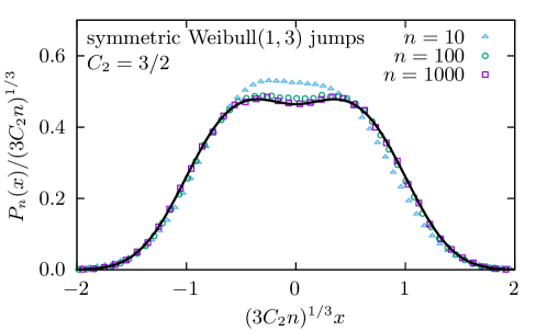
Figure 4: Case $p=2$. Comparison between the numerically obtained scaling function $F_{2}(z)$ and the prediction of Eq. (65). The scaling function is symmetric ($F_{2}(-z)=F_{2}(z)$), non-monotonic, with a pair of maxima at $z=\pm 0.350322\dots$ and a local minimum at $z=0$. The simulation data for $P_{n}(x)$, scaled as in (10), are shown with the symbols; they have been obtained with a normalized jump distribution of the symmetric Weibull type and shape factor $3$, i.e., $w(\eta)=\frac{3}{2}\,\eta^{2}\,e^{-|\eta|^{3}}$, thus $C_{2}=3/2$. The agreement for $n=1000$ is excellent. Measurements obtained from $10^{7}$ independent runs with $n=1000$ jumps each. Here again, the asymmetry that is visible at $n=10$ stems from our initial condition. Asymmetry is gradually washed out as time proceeds.

To fix $B_{2}$, we need to find the asymptotic behavior of ${}_{1}F_{1}(a,b,-x)$ when $x$ approaches $\infty$ along the real line and $\theta=a-b$ is a non-integer. It turns out that this asymptotic behavior is rather subtle and has been obtained only rather recently Paris (2013). For large $x$ one gets

$${}_{1}F_{1}(a,b,-x)=\frac{x^{-a}\,\Gamma(b)}{\Gamma(b-a)}\sum_{k=0}^{\infty}\frac{(a)_{k}\,(1+a-b)_{k}}{k!\,x^{k}}+x^{a-b}\,e^{-x}\left[\cos(\pi(a-b))\ +O(1/x)\right]\,,$$ (61)

where $(a)_{k}=\Gamma(a+k)/\Gamma(a)$ is the Pochamer symbol. Thus, generically, to leading order, it decays as a power law $\sim x^{-a}$ as $x\to\infty$. Substituting this asymptotic behavior in (60) using $x=8z^{3}/9$, we get as $z\to\infty$

$$F_{2}(z) \approx A_{1}\,\left[\frac{\Gamma(5/3)}{\Gamma(1/2)}\left(-\frac{8}{9}\right)^{-7/6}\left(B_{2}-\frac{\pi}{3\Gamma^{2}(5/6)}\,\left(\frac{2}{3}\right)^{1/3}\right)\,z^{-3/2}\,\sum_{k=0}^{\infty}\frac{9^{k}\,\Gamma(1/2+k)\Gamma(7/6+k)}{k!\,8^{k}\,z^{3k}}\right]$$ (62)

$$+ A_{1}\,\frac{\Gamma(1/3)\cos(\pi/6)}{\sqrt{\pi}}\,\left(\frac{8}{9}\right)^{1/6}\,z^{1/2}\,e^{-8z^{3}/9}\,.$$

Since the boundary condition for large $z$ predicts that $F_{2}(z)\sim\exp[-8z^{3}/9]$ (see Eq. (42)), we must eliminate the slow power law decay in (62). This can be done by choosing the constant $B_{2}$ as

$$B_{2}=\frac{\pi}{3\Gamma^{2}(5/6)}\,\left(\frac{2}{3}\right)^{1/3}\,.$$ (63)

Finally, the global constant $A_{1}$ is obtained from the normalization condition $\int_{0}^{\infty}F_{2}(z)\,dz=1/2$. This gives (upon using Mathematica to do the integral)

$$A_{1}=\left(\frac{3}{2}\right)^{1/3}\frac{\Gamma^{2}(5/6)}{\pi}\,.$$ (64)

Thus, with the two unknown constants $A_{1}$ and $B_{2}$ fixed, we then have our exact scaling function valid for all $z\geq 0$ (and symmetrically for $z\leq 0$)

$$F_{2}(z)=\left(\frac{3}{2}\right)^{1/3}\frac{\Gamma^{2}(5/6)}{\pi}\,{}_{1}F_{1}\left(\frac{1}{2},\frac{1}{3},-\frac{8z^{3}}{9}\right)+\frac{z^{2}}{3}\,{}_{1}F_{1}\left(\frac{7}{6},\frac{5}{3},-\frac{8z^{3}}{9}\right)\,.$$ (65)

The function $F_{2}(z)$ has the following asymptotic behaviors

$$F_{2}(z)\approx\begin{cases}\left(\frac{3}{2}\right)^{1/3}\frac{\Gamma^{2}(5/6)}{\pi}+\frac{1}{3}\,z^{2}+O(z^{3})&{\rm as}\,\,z\to 0\\ \\ b\,\sqrt{z}\,e^{-8z^{3}/9}&{\rm as}\,\,z\to\infty\end{cases}$$ (66)

where the constant prefactor $b$ is given by

$$b=\frac{\sqrt{3}}{2^{5/6}\,\pi^{3/2}}\,\Gamma^{2}(5/6)\,\Gamma(1/3)=0.595887\ldots$$ (67)

The large $z$ asymptotic follows from the remaining nonzero term in (62) once $B_{2}$ is fixed. One can check that the small $z$ behavior above is also completely in agreement with (43). A plot of this function $F_{2}(z)$ vs. $z$ is given in Fig. 4. In this Figure, we also compare our theoretical prediction with numerical simulations for $p=2$, finding excellent agreement. Interestingly, the function $F_{2}(z)$ is non-monotonic, and has a pair of maxima at $z\approx\pm 0.350322\dots$. The reason behind this non monotonicity has been put forward below Eq. (43): $p>1$ penalizes small jumps. Here, we consequently expect the dynamics to proceed in back and forth motion, from the left of the minimum to the right, and vice-versa for the subsequent successful jump. Such an oscillatory motion is fully compatible with the “two hump” structure of the scaling function for $p>1$. Yet, we stress that this oscillatory motion towards $x=0$ is not specific to cases with $p>1$: the late-time probability that the position changes sign after an accepted move is smoothly increasing when $p$ increases. This probability is given by

$$\frac{\int_{x}^{2x}\eta^{p}\,d\eta}{\int_{0}^{2x}\eta^{p}\,d\eta}\,=\,1-\frac{1}{2^{p+1}}.$$ (68)

Starting from 0 when $p\to-1^{+}$, it thus crosses 50% for $p=0$, and exceeds 90% for for $p>2.33$.

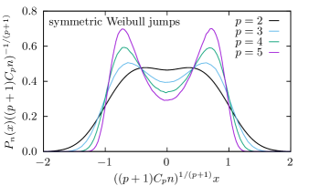
Figure 5: Numerically obtained asymptotic scaling functions $F_{p}(z)$ vs the scaling variable $z$ for $p=3,4,5$. The Monte Carlo simulations were run with a normalized jump distribution of the symmetric Weibull type and shape factor $(p+1)$, i.e., $w(\eta)=\frac{p+1}{2}\,\eta^{p}\,e^{-|\eta|^{p+1}}$. Measurements are collected over $10^{6}$ independent runs with $n=10^{5}$ jumps for $p=3,4$ and $n=10^{6}$ jumps for $p=5$. The curve for $p=2$ is Eq. (65) shown for comparison.

Finally, we show in Fig. 5 the evolution of the scaling function $F_{p}$ with $p$, as obtained in Monte Carlo simulations. The two hump structure resulting from increasing $p$ is visible. It is a consequence of the reduced likelihood of performing small jumps, when $p$ increases, as discussed at the end of section III.

V Concluding remarks

We have studied a stochastic steepest-gradient descent on a line, in a potential landscape $U(x)$. A random walker proceeds in discrete time, with a succession of jumps ($\eta_{n}$ at time $n$). The walker is greedy, in the sense that it only performs moves that decrease the energy $U(x)$. The dynamics does not depend on $U(x)$, and is driven to its minimum at $x=0$, irrespective of the value (or even the existence) of the gradient, as long as the minimum is non-degenerate (no local minima). The long-time regime has been shown to be self-similar, with a scaling function $F_{p}(z)$ that only depends on the likelihood of small jump displacements, through the parameter $p$: Denoting the jump probability distribution by $w(\eta)$, we have $w(\eta)\propto\eta^{p}$ for $\eta\to 0$ (and thus $p=0$ when $w(0)$ is finite). A Poisson-type of argument reveals that the large $z$ tail of the scaling function is of the form $\log F_{p}(z)\propto-z^{1+p}$, and it also provides the scaling variable as $z=x\,n^{1/(1+p)}$. In other words, the root mean squared (r.m.s.) spread of the particle’s position shrinks at large times $n$ as $n^{-1/(1+p)}$. It is quite natural that large $p$ values lead to a dynamical slow down, since they are associated to a smaller likelihood of small jumps, which is detrimental to evolution. A byproduct of the analysis is that redefining the clock from $n$ to $\cal N$, where $\cal N$ would count the number of accepted moves, the scaling variable would become $z={\cal N}x$, while the form of the scaling function $F_{p}$ would of course be unaffected.

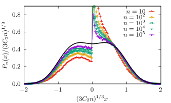
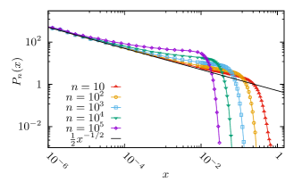
Figure 6: Monte Carlo results for initial conditions with a singularity at $x=0$, here $P_{0}(x)=\frac{1}{2}x^{-1/2}$ for $0<x<1$, and $P_{0}(x)=0$ otherwise; the jumps are of the symmetric Weibull type ($p=2$). The left panel shows the measured $P_{n}(x)$ after $n$ jumps averaged over $10^{7}$ realizations and scaled to demonstrate the slow convergence towards the scaling form $F_{2}(z)$ shown as a black line. The right panel shows $P_{n}(x)$ on a log-log scale, as a function of the unscaled variable $x$. Comparison of the two panels shows that close to $x=0$, $P_{n}(x)$ is of the form $x^{-1/2}$, before it crosses over to the asymptotic shape, further away from $x=0$.

We restricted the analysis to the search of the large-time symmetric scaling solution, which is universal in the sense that it is independent of initial conditions. The excellent agreement with the Monte Carlo simulations, that start from a non symmetric initial configuration, proves that asymmetric modes must decay faster than the symmetric ones. In some situations, the decay is slow. Such is the case when the initial distribution $P_{0}(x)$ is of the type $x^{-\mu}$ for small $x$ with $0<\mu<1$, thus singular near the origin. By construction, the smaller an $x$-value, the least probable it will be affected by the dynamics. We then expect that in such a case, $P_{n}(x)$ features the same singularity as $P_{0}(x)$ close enough to $x=0$. This is confirmed by Fig. 6, where $\mu=1/2$. The initial asymmetry of $P_{0}(x)$ (note that $P_{0}(x)=0$ for $x<0$), impinges on later times, while the singularity at $x=0$ has a rather spectacular effect on $P_{n}(x)$. Yet, Fig. 6 gives credit to the statement that for $n\ \to\infty$, the scaled $P_{n}$ tends towards $F_{2}$, as given in Eq. (60). In addition, explicit exact calculations for the double exponential jump distribution, beyond scaling, show 1) the convergence towards the symmetric scaling form and 2) the faster decay of asymmetric contributions coming from the initial conditions. Details are provided in Appendix B.

We did not discuss the cases where $w(\eta)$ is depleted near $\eta=0$, with a vanishing probability in some interval $[-\eta^{*},\eta^{*}]$: such a case would be non self-averaging, and lead to a dynamical arrest, whenever the walker arrives within the depletion segment $[-\eta^{*},\eta^{*}]$. One would need to average over may realizations sharing the same initial conditions in order to obtain an interesting a smooth late-time dynamics, where $P_{n}(x)\to\delta(x)$, thereby resolving the structure of the $\delta$ peak. Conversely, in the case we have studied, and although we have averaged our Monte Carlo data over a large number of samples to garner statistics, the dynamics is self-averaging in the sense that a single trajectory leads to a well defined scaling function; statistics is increased by following the evolution on longer time scales.

In this paper, we focused on $T=0$ where the steady state is trivial, but the late time relaxational dynamics is self-similar and typical observables (such as the r.m.s displacement) decay as a power law in time $n$ for large $n$. This power law behavior is due to the vanishing acceptance probability of new moves at the minimum. In a recent paper the authors (2021), we studied the finite temperature version of this model where the dynamics satisfies detailed balance. In this case the steady state is of Gibbs-Boltzmann form and the relaxation of observables towards their steady state value becomes exponential with the error due to incomplete convergence decaying as $\Lambda^{n}$ (with $\Lambda<1$). The relaxation time $\tau=-1/\ln\Lambda$ has a rich behavior as a function of the jump amplitude $a$, achieving a minimum value at an optimal $a^{*}$. Surprisingly for $a>a^{*}$, the relaxation at finite temperature is governed by self-similar scaling solutions very similar to the scaling ansatz established here for $T=0$. The framework developed here may thus find applications beyond the $T=0$ limit.

Appendix A Monte Carlo simulations

The zero temperature dynamics investigated here defines a Markov chain, that is naturally simulated with the Monte Carlo technique Frenkel and Smith (2002); Newman and Barkema (1999); Krauth (2006). In order to observe the relaxation of the particle distribution $P_{n}(x)$ we directly simulate $m$ independent particles (here $m=10^{6}$ or $m=10^{7}$), all starting at $x_{0}=-1$ by iterating

$$x_{n}=\begin{cases}x_{n-1}+\eta_{n}&{\rm if}\,\,\left|x_{n-1}+\eta_{n}\right|<\left|x_{n-1}\right|\\ x_{n-1}&{\rm otherwise},\end{cases},$$ (69)

which is a simplified but equivalent version of Eq. (1) using Eq. (4). The $\eta_{n}$ are independent random numbers drawn from the respective distributions $w(\eta)$, which (except for the Gaussian for which we used an implementation of the Ziggurat method Marsaglia et al. (2000)) can be generated using the inversion method Press et al. (2007). For each value of $n$ in which we are interested, e.g., $n=10,100,1000$, we initialize a histogram and update it with the position of the $m$ particles, after iteration $n$. We use the shape of the distribution we measured this way at different values of $n$ to determine whether our Markov chain is long enough to reach the predicted scaling form, which typically happens very fast for jump distributions with low values of $p$ and takes a longer time for jump distributions with larger values of $p$.

Appendix B An exact solution for the double-exponential jump distribution

To find a case where the long time asymptotic properties of the probability distribution $P_{n}(x)$ can be obtained exactly, we use the $p=0$ type jump distribution:

$$w(\eta)=\frac{1}{2}e^{-|\eta|}.$$ (70)

It is convenient to separate $P_{n}(x)$ into symmetric and anti-symmetric components:

$$P_{n}(x)=S_{n}(x)+Z_{n}(x)$$ (71)

with $S_{n}(x)=S_{n}(-x)$ and $Z_{n}(x)=-Z_{n}(-x)$. Substituting this decomposition in the Master equation (5) and using the symmetry of $w(\eta)$, one finds that the associated Master equations for $S_{n}$ and $Z_{n}$ separate. We first focus on the symmetric component $S_{n}(x)$. For $x>0$, the corresponding Master equation reads:

$$S_{n+1}(x)=\cosh(x)\int_{x}^{\infty}e^{-y}S_{n}(y)dy+R(x)S_{n}(x)$$ (72)

where we introduced a compact notation for the probability to reject an attempted move from $x$:

$$R(x)=\int_{-\infty}^{\infty}dy\,w(y-x)\,\theta\left(|y|-|x|\right)=e^{-x}\cosh x.$$ (73)

This quantity ranges from 1 at small $x$ (where most moves are rejected), to 1/2 at large $x$, where downhill moves only are accepted.

Introducing the generating function:

$$Q_{s}(x)=\sum_{n\geq 0}s^{n}S_{n}(x),$$ (74)

we find the equation:

$$\cosh(x)\int_{x}^{\infty}e^{-y}Q_{s}(y)dy+(e^{-x}\cosh x)Q_{s}(x)=\frac{Q_{s}(x)-S_{0}(x)}{s}.$$ (75)

This integral equation can be reduced to a first order differential equation, that can be integrated explicitly:

$$Q_{s}(x)=\frac{S_{0}(x)}{1-se^{-x}\cosh x}+2s(e^{2x}+e^{4x})h_{s}(x)^{-1-\frac{1}{2-s}}\int_{x}^{\infty}dy\;h_{s}(y)^{-1+\frac{1}{2-s}}S_{0}(y),$$ (76)

where we introduced the notation:

$$h_{s}(x) =e^{2x}(2-s)-s.$$ (77)

With this expression, we can use the general technique of singularity analysis Flajolet and Sedgewick (2009) to obtain exact results on the large $n$ behavior of $S_{n}(x)$, scrutinizing the complex plane position of the singularities of the generating function $Q_{s}(x)$ as function of the parameter $s$.

To make further progress, we assume $S_{0}(x)=\delta(|x|-y)/2$ (with $y>0$). This choice is the symmetric part of $P_{0}(x)=\delta(x-y)$ and we find:

$$2Q_{s}(x)=\frac{\delta(x-y)}{1-se^{-y}\cosh y}+2s(e^{2x}+e^{4x})h_{s}(x)^{-1-\frac{1}{2-s}}\;h_{s}(y)^{-1+\frac{1}{2-s}}\theta(y-x).$$ (78)

Singularities appear when $h_{s}(x)=0$ or $h_{s}(y)=0$. For $x<y$, the singularity in the complex $s$-plane that is closest to the origin $|s|=0$ is the solution of $h_{s}(x)=0$, and reads

$$s=\frac{2}{1+e^{-2x}}=R(x)^{-1}.$$ (79)

This implies that up to sub-exponential factors:

$$S_{n}(x)\sim R(x)^{n}.$$ (80)

Particles cannot climb uphill in this model and $R(x^{\prime})<R(x)$ for $x^{\prime}>x>0$. It is thus not surprising that the decay rate of $S_{n}(x)$ is determined by the rejection probability $R(x)$.

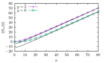
Figure 7: Comparison between the asymptotic behavior $2S_{n}(0)$ and numerical simulations for $S_{0}(x)=\delta(|x|-y)/2$, with $y=2$ and $y=6$. Symbols show numerical results and continuous black lines show Eq. (82).

It is possible to obtain sub-exponential corrections for particular values of $x$. For example for $x=0$, the singularity with the smallest modulus is at $s=1$. Expanding the generating function around this position, we find:

$$2Q_{s}(0)\simeq\frac{1}{(1-s)^{2}}-\frac{1}{1-s}\log\frac{1}{1-s}-\frac{1+\log(e^{2y}-1)/2}{1-s}+...$$ (81)

This allows us to obtain the sub-exponential corrections up to the first term that depends on the initial position $y$:

$$2S_{n}(0)\simeq n-\log n-\left(1+\gamma-\log 2+\log[e^{2y}-1]\right)+...,$$ (82)

where $\gamma$ is the Euler-Mascheroni constant. This formula is in good agreement with numerical simulations which are shown shown in Fig. (7) for two different initial positions $y$ of the random walker.

A similar asymptotic analysis for $x\ll 1$ gives:

$$2S_{n}(x)\simeq n^{1+x}R(x)^{n}+...,$$ (83)

where we derived only the leading sub-exponential term. Setting ${\widetilde{x}}=nx$, we can get:

$$S_{n}(n^{-1}{\widetilde{x}})\,\simeq\,\frac{n}{2}\left(1-\frac{|{\widetilde{x}}|}{n}\right)^{n}\,\simeq\,\frac{n}{2}\,e^{-|{\widetilde{x}}|}.$$ (84)

Using the result $F_{0}(z)=e^{-2z}$ derived in section IV.1 for the present $p=0$ situation, together with the fact that here, $C_{0}=B=1/2$, we recover the limiting scaling behaviour derived in section IV.1: $P_{n}(x)=nF_{0}(nx/2)/2$, see Eq. (46).

For the anti-symmetric component of the probability distribution $Z_{n}(x)$, the Master equation for $x>0$ is:

$$Z_{n+1}(x)=\sinh(x)\int_{x}^{\infty}e^{-y}Z_{n}(y)dy+R(x)Z_{n}(x).$$ (85)

As previously, we introduce the generating function: $\displaystyle K_{s}(x)=\sum_{n\geq 0}Z_{n}(x)s^{n},$ and obtain

$$K_{s}(x)=\frac{Z_{0}(x)}{1-se^{-x}\cosh x}+4se^{x}\sinh x\;h_{s}(x)^{\frac{1}{-2+s}}\int_{x}^{\infty}e^{\frac{2(1-s)y}{2-s}}h_{s}(y)^{-2+\frac{1}{2-s}}Z_{0}(y)dy.$$ (86)

Focusing on the choice $P_{0}(x)=\delta(x-y)$, we set $Z_{0}(x)=\left[\delta(x-y)-\delta(x+y)\right]/2$. For $0<x<y$, the position of the singularity with the smallest modulus lies at the same position as for the symmetric part: $s=R(x)^{-1}$. It is thus the sub-exponential factors that discriminate the decay rates of the symmetric and anti-symmetric components. Expanding the generating function to first order around $x=0$ near the pole at $s=1$, we find:

$$K_{s}(x) \simeq\frac{x(\coth y-1)}{1-s}.$$ (87)

This gives the expected small $x$ asymptotic behavior for $Z_{n}(x)$:

$$Z_{n}(x) \simeq x(\coth y-1).$$ (88)

This confirms that the antisymmetric component is indeed negligible, in the large $n$ limit, against its symmetric counterpart: $|Z_{n}(x)|\ll S_{n}(x)$, for small enough $|x|$. This stems from the additional $h_{s}(x)^{-1}$ factor present in Eq. (76), as compared to Eq. (86).

References

- Cauchy (1847) A. Cauchy, Applied Mathematical Sciences 25, 536 (1847).
- Robbins and Monro (1951) H. Robbins and S. Monro, The Annals of Mathematical Statistics 22, 400 (1951).
- Spall (2012) J. C. Spall, “Stochastic optimization,” in Handbook of Computational Statistics: Concepts and Methods, edited by J. E. Gentle, W. K. Härdle, and Y. Mori (Springer Berlin Heidelberg, Berlin, Heidelberg, 2012) p. 173.
- Sra et al. (2011) S. Sra, S. Nowozin, and S. J. Wright, Optimization for Machine Learning (The MIT Press, 2011).
- Frenkel and Smith (2002) D. Frenkel and B. Smith, Understanding Molecular Simulations, 2nd ed. (Adademic Press, 2002).
- Newman and Barkema (1999) M. E. J. Newman and G. T. Barkema, Monte Carlo Methods in Statistical Physics (Oxford University Press, 1999).
- Krauth (2006) W. Krauth, Statistical Mechanics: Algorithms and Computations (Oxford Master Series in Physics, 2006).
- Note (1) The limit is not innocuous, for it breaks detailed balance Monthus.
- (9) W. R. Inc., “Mathematica, Version 12.3,” .
- Paris (2013) R. B. Paris, Applied Mathematical Sciences 7, 6601 (2013).
- the authors (2021) the authors, in preparation (2021).
- Marsaglia et al. (2000) G. Marsaglia, W. W. Tsang, et al., Journal of statistical software 5, 1 (2000).
- Press et al. (2007) W. H. Press, H. William, S. A. Teukolsky, W. T. Vetterling, A. Saul, and B. P. Flannery, Numerical recipes 3rd edition: The art of scientific computing (Cambridge university press, 2007).
- Flajolet and Sedgewick (2009) P. Flajolet and R. Sedgewick, Analytic Combinatorics (Cambridge University Press, 2009).