RelaySum for Decentralized Deep Learning
on Heterogeneous Data

Abstract

In decentralized machine learning, workers compute model updates on their local data. Because the workers only communicate with few neighbors without central coordination, these updates propagate progressively over the network. This paradigm enables distributed training on networks without all-to-all connectivity, helping to protect data privacy as well as to reduce the communication cost of distributed training in data centers. A key challenge, primarily in decentralized deep learning, remains the handling of differences between the workers’ local data distributions. To tackle this challenge, we study the RelaySum mechanism for information propagation in decentralized learning. RelaySum uses spanning trees to distribute information exactly uniformly across all workers with finite delays depending on the distance between nodes. In contrast, the typical gossip averaging mechanism only distributes data uniformly asymptotically while using the same communication volume per step as RelaySum. We prove that RelaySGD, based on this mechanism, is independent of data heterogeneity and scales to many workers, enabling highly accurate decentralized deep learning on heterogeneous data. Our code is available at http://github.com/epfml/relaysgd.

1 Introduction

Ever-growing datasets lay at the foundation of the recent breakthroughs in machine learning. Learning algorithms therefore must be able to leverage data distributed over multiple devices, in particular for reasons of efficiency and data privacy. There are various paradigms for distributed learning, and they differ mainly in how the devices collaborate in communicating model updates with each other. In the all-reduce paradigm, workers average model updates with all other workers at every training step. In federated learning [24], workers perform local updates before sending them to a central server that returns their global average to the workers. Finally, decentralized learning significantly generalizes the two previous scenarios. Here, workers communicate their updates with only few directly-connected neighbors in a network, without the help of a server.

Decentralized learning offers strong promise for new applications, allowing any group of agents to collaboratively train a model while respecting the data locality and privacy of each contributor [25]. At the same time, it removes the single point of failure in centralized systems such as in federated learning [12], improving robustness, security, and privacy. Even from a pure efficiency standpoint, decentralized communication patterns can speed up training in data centers [2].

In decentralized learning, workers share their local stochastic gradient updates with the others through gossip communication [41]. They send their updates to their neighbors, which iteratively propagate the updates further into the network. The workers typically use iterative gossip averaging of their models with their neighbors, using averaging weights chosen to ensure asymptotic uniform distribution of each update across the network. It will take $\tau$ rounds of communication for an update from worker $i$ to reach a worker $j$ that is $\tau$ hops away, and when it first arrives, the update is exponentially weakened by repeated averaging with weights $<1$. In general networks, worker $j$ will never exactly, but only asymptotically receive its uniform share of the update. The slow distribution of updates not only slows down training, but also makes decentralized learning sensitive to heterogeneity in workers’ data distributions.

We study an alternative mechanism to gossip averaging, which we call RelaySum. RelaySum operates on spanning trees of the network, and distributes information exactly uniformly within a finite number of gossip steps equal to the diameter of the network. Rather than iteratively averaging models, each node acts as a ‘router’ that relays messages through the whole network without decaying their weight at every hop. While naive all-to-all routing requires $n^{2}$ messages to be transmitted at each step, we show that on trees, only $n$ messages (one per edge) are sufficient. This is enabled by the key observation that the routers can merge messages by summation to avoid any extra communication compared to gossip averaging. RelaySum achieves this using additional memory linear in the number of edges, and by tailoring the messages sent to different neighbors. At each time step, RelaySum workers receive a uniform average of exactly one message from each worker. Those messages just originate from different time delays depending on how many hops they travelled. The difference between gossip averaging and RelaySum is illustrated in Figure 1.

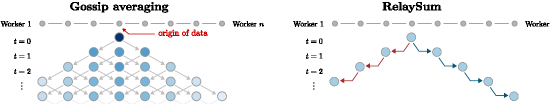
Figure 1: To spread information across a decentralized network, classical gossip averaging diffuses information slowly through the network. The left figure illustrates the spread of information originating from the fourth worker in a chain network. In RelaySum, the messages are relayed without reweighting, resulting in uniform delivery of the information to every worker. When multiple workers broadcast simultaneously (not pictured), RelaySum can sum their messages and use the same bandwidth as gossip averaging.

The RelaySum mechanism is structurally similar to Belief Propagation algorithms for inference in graphical models. This link was made by Zhang et al. [50], who used the same mechanism for decentralized weighted average consensus in control.

We use RelaySum in the RelaySGD learning algorithm. We theoretically show that this algorithm is not affected by differences in workers’ data distributions. Compared to other algorithms that have this property [36, 31], RelaySGD does not require the selection of averaging weights, and its convergence does not depend on the spectral gap of the averaging matrix, but instead on the network diameter.

While RelaySum is formulated for trees, it can be used in any decentralized network. We use the Spanning Tree Protocol [30] to construct spanning trees of any network in a decentralized fashion. RelaySGD often performs better on any such spanning tree than gossip-based methods on the original graph. When the communication network can be chosen freely, the algorithm can use double binary trees [33]. While these trees have logarithmic diameter and scale to many workers, RelaySGD in this setup uses only constant memory equivalent to two extra copies of the model parameters and sends and receives only two models per iteration.

Surprisingly, in deep learning with highly heterogeneous data, prior methods that are theoretically independent of data heterogeneity [36, 31], perform worse than heuristic methods that do not have this property, but use cleverly designed time-varying communication topologies [2]. In extensive tests on image- and text classification, RelaySGD performs better than both kinds of baselines at equal communication budget.

2 Related work

Out of the multitude of decentralized optimization methods, first-order algorithms that interleave local gradient updates with a form of gossip averaging [29, 11] show most promise for deep learning. Such algorithms are theoretically analyzed for convex and non-convex objectives in [28, 11, 29], and [19, 36, 2, 20] demonstrate that gossip-based methods can perform well in deep learning.

In a gossip averaging step, workers average their local models with the models of their direct neighbors. The corresponding ‘mixing matrix’ is a central object of study. The matrix can be doubly-stochastic [29, 19, 16], column-stochastic [38, 26, 39, 2], row-stochastic [40, 44], or a combination [42, 43, 32]. Column-stochastic methods use the push-sum consensus mechanism [13] and can be used on directed graphs. Our analysis borrows from the theory developed for those methods.

While gossip averages in general requires an infinite number of steps to reach exact consensus, another line of work identifies mixing schemes that yield exact consensus in finite steps. For some graphs, this is possible with time-independent averaging weights [15, 6]. One can also achieve finite-time consensus with time-varying mixing matrices. On trees, for instance, exact consensus can be achieved by routing updates to a root node and back, in exactly diameter number of steps [15, 6]. On some graphs, tighter bounds can be established [8]. For fully-connected networks with $n$ workers, Assran et al. [2] design a sparse time-varying communication scheme that yields exact consensus in a cycle of $\log n$ averaging steps and performs well in deep learning.

The ‘relay’ mechanism of RelaySGD was previously used by Zhang et al. [50] in the control community for the decentralized weighted average consensus problem, but they do not use it in the context of optimization. Zhang et al. also introduce a modified algorithm for loopy graphs, but this modification makes the achieved consensus inexact. The ‘relay’ mechanism effectively turns a sparse graph into a fully-connected graph with communication delays. Work on delayed consensus [27] and optimization [37, 1] analyzes such schemes for centralized distributed algorithms. Those consensus schemes are, however, not directly applicable to decentralized optimization.

A fundamental challenge in decentralized learning is dealing with data that is not identically distributed among workers. Because, in this case, workers pursue different optima, workers may drift [29] and this can harm convergence. There is a large family of algorithms that introduce update corrections that provably mitigate such data heterogeneity. Examples applicable to non-convex problems are exact diffusion [45], Gradient Tracking [22, 31, 48], D² [36], PushPull [32]. To tackle the same challenge, Lin et al. [20], Yuan et al. [46] propose modifications to local momentum to empirically improve performance in deep learning, but without provable guarantees. Lu and De Sa [23] propose DeTAG which overlaps multiple consecutive gossip steps and gradient computations to accelerate information diffusion. This technique could be applied to the RelaySum mechanism, too.

3 Method

Setup

We consider standard decentralized optimization with data distributed over $n\geq 1$ nodes:

$$\textstyle f^{\star}:=\min_{\mathbf{x}\in\mathbb{R}^{d}}\left[f(\mathbf{x})=\frac{1}{n}\sum_{i=1}^{n}\left[f_{i}(\mathbf{x}):=\operatorname{\mathbb{E}}_{\xi\sim\mathcal{D}_{i}}F_{i}(\mathbf{x},\xi_{i})\right]\right]\,.$$

Here $\mathcal{D}_{i}$ denotes the distribution of the data on node $i$ and $f_{i}\colon\mathbb{R}^{d}\to\mathbb{R}$ the local optimization objectives. Workers are connected by a network respecting a graph topology $\mathcal{G}=(\mathcal{V},\mathcal{E})$, where $\mathcal{V}=\{1,\ldots,n\}$ denotes the set of workers, and $\mathcal{E}$ the set of undirected communication links between them (without self loops). Each worker $i$ can only directly communicate with its neighbors $\mathcal{N}_{i}\subset\mathcal{V}$.

Decentralized learning with gossip

We consider synchronous first-order algorithms that interleave local gradient-based updates

$$\mathbf{x}_{i}^{(t+\nicefrac{{1}}{{2}})}=\mathbf{x}_{i}^{(t)}+\mathbf{u}_{i}^{(t)}$$

with message exchange between connected workers. For SGD with typical gossip averaging (DP-SGD [19]), the local updates can be written as $\mathbf{u}_{i}^{(t)}=-\gamma\nabla f_{i}(\mathbf{x}_{i}^{(t)},\xi_{i}^{(t)})$, and the messages exchanged between pairs of connected workers $(i,j)$ are $\mathbf{m}_{i\to j}^{(t)}=\mathbf{x}_{i}^{(t+\nicefrac{{1}}{{2}})}\in\mathbb{R}^{d}$. Each timestep, the workers average their model with received messages,

$$\textstyle\mathbf{x}_{i}^{(t+1)}=\mathbf{W}_{ii}\mathbf{x}_{i}^{(t+\nicefrac{{1}}{{2}})}+\sum_{j\in\mathcal{N}_{i}}\mathbf{W}_{ij}\mathbf{m}_{j\to i}^{(t)},$$ (DP-SGD)

using averaging weights defined by a gossip matrix $\mathbf{W}\in\mathbb{R}^{n\times n}$.

In this scheme, an update $\mathbf{u}_{i}^{(t_{1})}$ from any worker $i$ will be linearly incorporated into the model $\mathbf{x}_{j}^{(t_{2})}$ at a later timestep $t_{2}$ with weight $(\mathbf{W}^{t_{2}-t_{1}})_{ij}$. The gossip matrix must be chosen such that these weights asymptotically converge to $\frac{1}{n}$, distributing all updates uniformly over the workers. This setup appears in, for example, [19, 16].

Uniform model averaging

If the graph topology is fully-connected, any worker can communicate with any other worker, and it is ideal to use ‘all-reduce averaging’,

$$\textstyle\mathbf{x}_{i}^{(t+1)}=\frac{1}{n}\sum_{j=1}^{n}\mathbf{x}_{j}^{(t+\nicefrac{{1}}{{2}})}.$$

Contrary to the decentralized scheme (DP-SGD), this algorithm does not degrade in performance if data is distributed heterogeneously across workers. In sparsely connected networks, however, all-reduce averaging requires routing messages through the network. On arbitrary networks, such a routing protocol requires at least a number of communication steps equal to the network diameter $\tau_{\text{max}}$—the minimum number of hops some messages have to travel.

RelaySGD

In this paper, we approximate the all-reduce averaging update as

$$\textstyle\mathbf{x}_{i}^{(t+1)}=\frac{1}{n}\sum_{j=1}^{n}\mathbf{x}_{j}^{(t-\tau_{ij}+\nicefrac{{1}}{{2}})},$$ (RelaySGD)

where $\tau_{ij}$ is minimum number of network hops between workers $i$ and $j$ (and $\tau_{ii}=0$). Since it takes $\tau_{ij}$ steps to route a message from worker $i$ to $j$, this scheme could be implemented using a peer-to-peer routing protocol like Ethernet. Of course, this naive implementation drastically increases the bandwidth used compared to gossip averaging. The key insight of this paper is that, on tree networks, the RelaySGD update rule can be implemented while using the same communication volume per step as gossip averaging, using additional memory linear in the number of a worker’s direct neighbors.

RelaySum

To implement RelaySGD, we require a communication mechanism that delivers sums of delayed ‘parcels’ $s_{w}^{(t)}=\sum_{j=1}^{n}p_{j}^{(t-\tau_{wj})}$ to each worker $w$ in a tree network, where the parcel $p_{j}^{(t)}$ is created by worker $j$ at time $t$. To simplify the exposition, let us first consider the simplest type of tree network: a chain. In a chain, a worker $w$ is connected to workers $w-1$ and $w+1$, if those exist, and the delays are $\tau_{ij}=|i-j|$. We can then decompose

$$s_{w}^{(t)}=\sum_{j=1}^{n}p_{j}^{(t-\tau_{wj})}=p_{w}^{(t)}+\underbrace{\sum_{j=1}^{w-1}p_{j}^{(t-\tau_{wj})}}_{\text{parcels from the `left'}}+\underbrace{\sum_{j=w+1}^{n}p_{j}^{(t-\tau_{wj})}}_{\text{parcels from the `right'}}.$$

The sum of parcels from the ‘left’ will be sent as one message $m_{(w-1)\to w}$ from worker $w-1$ to $w$, and the sum of data from the ‘right’ will be sent as one message $m_{(w+1)\to w}$ from $w+1$ to $w$. Neighboring workers can compute these messages from the messages they received from their neighbors in the previous timestep. Compared to typical gossip averaging, RelaySum requires additional memory linear in the number of neighbors, but it uses the same volume of communication.

Algorithm 1 shows how this scheme is generalized to general tree networks and incorporated into RelaySGD. Along with the model parameters, we send scalar counters that are used in the first few iterations of the algorithm $t\leq\tau_{\text{max}}$ to correct for messages that have not yet arrived.

Algorithm 1 RelaySGD

1:$\forall~{}i,~{}\mathbf{x}_{i}^{(0)}=\mathbf{x}^{(0)}$; $\forall~{}i,j,\mathbf{m}^{(-1)}_{i\rightarrow j}=\mathbf{0}$, counts $c^{(-1)}_{i\rightarrow j}=0$, learning rate $\gamma$, tree network

2:for $t=0,1,\ldots$ do

3:     for node $i$ in parallel

4:         $\mathbf{x}^{(t+\nicefrac{{1}}{{2}})}_{i}=\mathbf{x}^{(t)}_{i}{\color[rgb]{0.121,0.466,0.705}-\gamma\nabla f_{i}(\mathbf{x}_{i}^{(t)})}$(or Adam/momentum)

5:         for each neighbor $j\in\mathcal{N}_{i}$ do

6:              Send $\mathbf{m}^{(t)}_{i\rightarrow j}=x_{i}^{(t+\nicefrac{{1}}{{2}})}{\color[rgb]{0.121,0.466,0.705}+\sum_{k\in\mathcal{N}_{i}\backslash j}\mathbf{m}^{(t-1)}_{k\rightarrow i}}$(relay messages from other neighbors)

7:              Send corresponding counters $c^{(t)}_{i\rightarrow j}=1+\sum_{k\in\mathcal{N}_{i}\backslash j}c^{(t-1)}_{k\rightarrow i}$

8:              Receive ($\mathbf{m}^{(t)}_{j\rightarrow i}$, $c^{(t)}_{j\rightarrow i}$) from node $j$

9:         end for

10:         $\bar{n}_{i}^{(t+1)}=1+\sum_{j\in\mathcal{N}_{i}}c^{(t)}_{j\rightarrow i}$ ($\bar{n}$ converges to the total number of workers)

11:         $\mathbf{x}_{i}^{t+1}=\frac{1}{\bar{n}_{i}^{(t+1)}}\left(\mathbf{x}_{i}^{(t+\nicefrac{{1}}{{2}})}+\sum_{j\in\mathcal{N}_{i}}\mathbf{m}^{(t)}_{j\rightarrow i}\right)$ $\left(=\frac{1}{n}\sum_{j=1}^{n}\mathbf{x}_{j}^{(t-\tau_{ij}+\nicefrac{{1}}{{2}})}\right)$

12:     end for

13:end for

Spanning trees

RelaySGD is formulated on tree networks, but it can be used on any communication graph by constructing a spanning tree. In a truly decentralized setting, we can use the Spanning Tree Protocol [30] used in Ethernet to find such trees in a decentralized fashion. The protocol elects a leader as the root of the tree, after which every other node finds the fastest path to this leader.

On the other hand, when the decentralized paradigm is used in a data center to reduce communication, RelaySGD can run on double binary trees [33] used in MPI and NCCL [10]. The key idea of double binary trees is to use two different communication topologies for different parts of the model. We communicate odd coordinates using a balanced binary tree $A$, and communicate the even coordinates with a complimentary tree $B$. The trees $A$ and $B$ are chosen such that internal nodes (with 3 edges) in one tree are leaves (with only 1 edge) in the other. Using the combination of two trees, RelaySGD requires only constant extra memory equivalent to at most 2 model copies (just like the Adam optimizer [14]), and it sends and receives the equivalent of 2 models (just like on a ring).

4 Theoretical analysis

Since RelaySGD updates worker’s models at time step $t+1$ using models from (at most) the past $\tau_{\max}$ steps, we conveniently reformulate RelaySGD in the following way: Let $\mathbf{Y}^{(t)},\mathbf{G}^{(t)}\in\mathbb{R}^{n(\tau_{\max}+1)\times d}$ denote stacked worker models and gradients whose row vectors at index $n\!\cdot\!\tau+i$ represent

$$\left[\mathbf{Y}^{(t)}\right]_{n\tau+i}^{\top}=\begin{cases}\mathbf{x}_{i}^{(t-\tau)}&t\geq\tau\\ \mathbf{x}^{(0)}&\text{otherwise}\end{cases},\qquad\left[\mathbf{G}^{(t)}\right]_{n\tau+i}^{\top}=\begin{cases}\nabla F_{i}(\mathbf{x}_{i}^{(t-\tau)};\xi_{i}^{(t-\tau)})&t\geq\tau\\ \mathbf{x}^{(0)}&\text{otherwise}\end{cases}$$

for all times $t\geq 0$, delay $\tau\in[0,\tau_{\max}]$ and worker $i\in[n]$. Then (RelaySGD) can be written as

$$\mathbf{Y}^{(t+1)}=\mathbf{W}\mathbf{Y}^{(t)}-\gamma\tilde{\mathbf{W}}\mathbf{G}^{(t)}$$

where $\mathbf{W},\tilde{\mathbf{W}}\in\mathbb{R}^{n(\tau_{\max}+1)\times n(\tau_{\max}+1)}$ are non-negative matrices whose elements are

$$\left[\mathbf{W}\right]_{n\tau+i,n\tau^{\prime}+j}=\begin{cases}\tfrac{1}{n}&\tau=0\text{ and }\tau^{\prime}=\tau_{ij}\\ 1&i=j\text{ and }\tau=\tau^{\prime}+1\\ 0&\text{otherwise}\end{cases},\qquad\left[\tilde{\mathbf{W}}\right]_{n\tau+i,n\tau^{\prime}+j}=\begin{cases}\tfrac{1}{n}&\tau=0\text{ and }\tau^{\prime}=\tau_{ij}\\ 0&\text{otherwise}\end{cases}$$

for all $\tau,\tau^{\prime}\in[0,\tau_{\max}]$ and $i,j\in[n]$. The matrix $\mathbf{W}$ can be interpreted as the mixing matrix of an ‘augmented graph’ [27] with additional virtual ‘forwarding nodes’. $\mathbf{W}$ is row stochastic and its largest eigenvalue is 1. The vector of all ones $\mathbf{1}_{n(\tau_{\max}+1)}\in\mathbb{R}^{n(\tau_{\max}+1)}$ is a right eigenvector of $\mathbf{W}$ and let $\bm{\pi}\in\mathbb{R}^{n(\tau_{\max}+1)}$ be the left eigenvector such that $\bm{\pi}^{\top}\mathbf{1}_{n(\tau_{\max}+1)}=1$.

We characterize the convergence rate of the consensus distance in the following key lemma:

Lemma 1 (Key lemma).

There exists an integer $m=m(\mathbf{W})>0$ such that for any $\mathbf{X}\in\mathbb{R}^{n(\tau_{\max}+1)\times d}$ we have

$$\|\mathbf{W}^{m}\mathbf{X}-\mathbf{1}\bm{\pi}^{\top}\mathbf{X}\|^{2}\leq(1-p)^{2m}\|\mathbf{X}-\mathbf{1}\bm{\pi}^{\top}\mathbf{X}\|^{2},$$

where $p=\frac{1}{2}(1-|\lambda_{2}(\mathbf{W})|)$ is a constant.

All the following optimization convergence results will only depend on the effective spectral gap $\rho:=\frac{p}{m}$ of $\mathbf{W}$. We empirically observe that $\rho=\Theta(1/n)$ for a variety of network topologies (see Figure 5 in Appendix A).

Remark 2.

The above key lemma is similar to [16, Assumption 4] for gossip-type averaging with symmetric matrices. However, in our case $\mathbf{W}$ is just a row stochastic matrix, and its spectral norm $\|\mathbf{W}\|_{2}>1$. In general, the consensus distance can increase after just one single communication step (multiplication by $\mathbf{W}$). That is why we need $m>1$. The proof of the Lemma relies on a Perron-Frobenius type theorem, and holds over several steps $m$ instead of a single iteration. It means RelaySum defines a consensus algorithm with linear convergence rate which pulls models closer.

Our main convergence results hold under the following common assumptions, as e.g. [16].

Assumption A (L-smoothness).

For each $i\in[n]$, $F_{i}(\mathbf{x},\xi):\mathbb{R}^{D}\times\Omega_{i}\rightarrow\mathbb{R}$ is differentiable for each $\xi\in\text{supp}(\mathcal{D}_{i})$ and there exists a constant $L\geq 0$ such that for each $\mathbf{x},\mathbf{y}\in\mathbb{R}^{d}$, $\xi\in\text{supp}(\mathcal{D}_{i})$:

$$\|\nabla F_{i}(\mathbf{x},\xi)-\nabla F_{i}(\mathbf{y},\xi)\|\leq L\|\mathbf{x}-\mathbf{y}\|\,.$$

Assumption B (Uniform bounded noise).

There exists constant $\bar{\sigma}$, such that for all $\mathbf{x}\in\mathbb{R}^{d}$, $i\in[n]$,

$$\operatorname{\mathbb{E}}_{\xi}\|\nabla F_{i}(\mathbf{x},\xi)-\nabla f_{i}(\mathbf{x})\|^{2}\leq\bar{\sigma}^{2}.$$

Assumption C ($\mu$-convexity).

For $i\in[n]$, each function $f_{i}:\mathbb{R}^{d}\rightarrow\mathbb{R}$ is $\mu$-(strongly) convex for constant $\mu\geq 0$. That is, $\forall~{}\mathbf{x},\mathbf{y}\in\mathbb{R}^{d}$

$$f_{i}(\mathbf{x})-f_{j}(\mathbf{y})+\tfrac{\mu}{2}\|\mathbf{x}-\mathbf{y}\|^{2}_{2}\leq\nabla f_{i}(\mathbf{x})^{\top}(\mathbf{x}-\mathbf{y})\,.$$

Theorem I (RelaySGD).

For any target accuracy $\varepsilon>0$ and an optimal solution $\mathbf{x}^{\star}$,

(Convex:) under Assumptions A, B and C with $\mu\geq 0$, it holds that $\tfrac{1}{T+1}\textstyle\sum\nolimits_{t=0}^{T}\left(f(\overline{\mathbf{x}}^{(t)})\!-\!f(\mathbf{x}^{\star})\right)\leq\varepsilon$ after

$$\textstyle\mathcal{O}\left(\frac{\bar{\sigma}^{2}}{n\varepsilon^{2}}+\frac{C\sqrt{L}\bar{\sigma}}{\varepsilon^{\nicefrac{{3}}{{2}}}}+\frac{CL}{\varepsilon}\right)R_{0}^{2}$$

iterations. Here $\overline{\mathbf{x}}^{(t)}\!:=\!\bm{\pi}^{\top}\mathbf{Y}^{(t)}$ averages past models, $R_{0}^{2}\!=\!\|\mathbf{x}^{0}-\mathbf{x}^{\star}\|^{2}$, and $C\!=\!\mathcal{O}(\frac{1}{\rho}\tau_{\max}^{\nicefrac{{3}}{{2}}})$. (Non-convex:) under Assumptions A and B, it holds that $\tfrac{1}{T+1}\textstyle\sum\nolimits_{t=0}^{T}\|\nabla f(\overline{\mathbf{x}}^{(t)})\|^{2}\leq\varepsilon$ after

$$\textstyle\mathcal{O}\left(\frac{\bar{\sigma}^{2}}{n\varepsilon^{2}}+\frac{C\bar{\sigma}}{\varepsilon^{\nicefrac{{3}}{{2}}}}+\frac{C}{\varepsilon}\right)LF_{0}$$

iterations, where $F_{0}:=f(\overline{\mathbf{x}}^{(0)})-f(\mathbf{x}^{\star})$.

The dominant term in our convergence result, $\mathcal{O}\bigl{(}\frac{\bar{\sigma}^{2}}{n\varepsilon^{2}}\bigr{)}$ matches with the dominant term in the convergence rate of centralized (‘all-reduce’) mini-batch SGD, and thus can not be improved.

In contrast to other methods, the presented convergence result of RelaySGD is independent of the data heterogeneity $\zeta^{2}$ in [16, Assumption 3b].

Definition D (Data heterogeneity).

There exists a constant $\zeta^{2}$ such that $\forall~{}i\in[n],\mathbf{x}\in\mathbb{R}^{d}$

$$\textstyle\|\nabla f_{i}(\mathbf{x})-\nabla f(\mathbf{x})\|_{2}^{2}\leq\zeta^{2}\,.$$

Remark 3.

For convex objectives, Assumptions B and D can be relaxed to only hold at the optimum $\mathbf{x}^{\star}$. A weaker variant of A only uses $L$-smoothness of $f_{i}$ [16, Assumption 1b].

Comparing to gossip averaging for convex $f_{i}$ which has complexity $\mathcal{O}(\tfrac{\bar{\sigma}^{2}}{n\varepsilon^{2}}+(\tfrac{\zeta}{\rho}+\tfrac{\bar{\sigma}}{\sqrt{\rho}})\frac{\sqrt{L}}{\varepsilon^{\nicefrac{{3}}{{2}}}}+\tfrac{L}{\rho\varepsilon})R_{0}^{2}\vspace{-1mm}$, our rate for RelaySGD does not depend on $\zeta^{2}$ and has same leading term $\mathcal{O}(\frac{\bar{\sigma}^{2}}{n\varepsilon^{2}})$ as $D^{2}$.

5 Experimental analysis and practical properties

5.1 Effect of network topology

Random quadratics

To efficiently investigate the scalability of RelaySGD with respect to the number of workers, and to study the benefits of binary tree topologies over chains, we introduce a family of synthetic functions. We study random quadratics with local cost functions $f_{i}(\mathbf{x})=\lVert\mathbf{A}_{i}\mathbf{x}-\mathbf{b}_{i}^{\top}\mathbf{x}\rVert^{2}$ to precisely control all constants that appear in our theoretical analysis. The Hessians $\mathbf{A}_{i}$ are initialized randomly, and their spectrum is scaled to achieve a desired smoothness $L$ and strong convexity $\mu$. The offsets $\mathbf{b}_{i}$ ensure a desired level of heterogeneity $\zeta^{2}$ and distance between optimum and initialization $r_{0}$. Appendix B.4 describes the generation of these quadratics in detail.

Scalability on rings and trees

Using these quadratics, Figure 2 studies the number of steps required to reach a suboptimality $f(\bar{\mathbf{x}})-f(\mathbf{x}^{\star})\leq\varepsilon$ with tuned constant learning rates. On ring topologies with uniform (1/3) gossip weights (and chains for RelaySum), all compared methods require steps at least linear in the number of workers to reach the target quality. RelaySGD and D² empirically scale significantly better than Gradient Tracking, these methods are all independent of data heterogeneity. On a balanced binary tree network with Metropolis-Hastings weights [41], both D² and Gradient Tracking notably do not scale better than on a ring, while RelaySGD on these trees requires only a number of steps logarithmic in the number of workers. SGP with their time-varying exponential topology scales well, too, but it requires more steps on more heterogeneously distributed data.

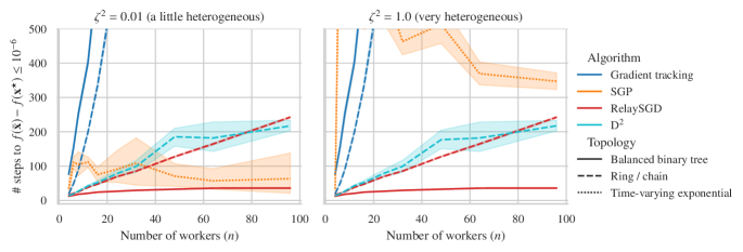
Figure 2: Time required to optimize random quadratics ($\sigma^{2}=0,r_{0}=10,L=1,\mu=0.5$) to suboptimality $\leq 10^{-6}$ with varying numbers of workers with tuned constant learning rates. On a ring ( ),  D² and  RelaySGD require steps linear in the number of workers, and this number is independent of the data heterogeneity. RelaySGD reduces this to $\log n$ on a balanced tree topology ( ), but trees do not improve  D² or  Gradient Tracking. For  SGP with time-varying exponential topology ( ), the number of steps does not consistently grow with more workers, but this number becomes higher with more heterogeneity (left v.s. right plot).

5.2 Spanning trees compared to other topologies

RelaySGD cannot utilize all available edges in arbitrary networks to communicate, but is restricted to a spanning tree of the graph. We empirically find that this restriction is not limiting. In Figure 3, we take an organic social network topology based on the Davis Southern Women graph [4] from NetworkX [7], and construct random spanning trees found by the Spanning Tree Protocol [30]. On any such spanning tree, RelaySGD optimizes random heterogeneous quadratics as fast as D² on the full graph with Metropolis-Hastings weights [41], significantly faster than DP-SGD.

For decentralized learning used in a fully-connected data center for communication efficiency, the deep learning experiments below show that RelaySGD on double binary trees outperforms the most popular non-tree-based communication scheme used in decentralized deep learning [2].

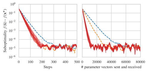
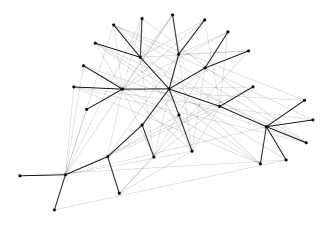
Figure 3: Performance of  RelaySGD on spanning trees of the Social Network graph (32 nodes) found using Spanning Tree Protocol, compared to  DP-SGD and  D² on the full network. Solid lines ( ) indicate spanning trees while dashed lines ( ) indicate the full graph. The figure on the right shows one spanning tree on top of the original network. Learning rates are tuned to reach suboptimality $\leq 10^{-5}$ on random quadratics ($\zeta^{2}=0.1,\sigma^{2}=0.1,r_{0}=1,L=1,\mu=0.5$).  RelaySGD on spanning trees converges as fast as  D² on the full network, while the total communication on spanning trees is smaller than on the full graph.

5.3 Effect of data heterogeneity in decentralized deep learning

We study the performance of RelaySGD in deep-learning based image- and text classification. While the algorithm is theoretically independent of dissimilarities in training data, other methods (D², RelaySGD/Grad) that have the same property often lose accuracy in the presence of high data heterogeneity [20]. To study the dependence of RelaySGD in practical deep learning, we partition training data strictly across 16 workers and distribute the classes using a Dirichlet process [47, 20]. The Dirichlet parameter $\alpha$ controls the heterogeneity of the data across workers.

We compare RelaySGD against a variety of other algorithms. DP-SGD [19] is the most natural combination of SGD with gossip averaging, and we chose D² [36] to represent the class of previous work that is theoretically robust to heterogeneity. We extend D² to allow varying step sizes and local momentum, according to Appendix D.4, and make it suitable for practical deep learning. Although Stochastic Gradient Push [2] is not theoretically independent of data heterogeneity, it is a popular choice in the data center setting, where they use a time-varying exponential scheme on $2^{d}$ workers that mixes exactly uniformly in $d$ rounds (Appendix D.6). We also compare to DP-SGD with quasi-global momentum [20], a practical method recently introduced to increase robustness to heterogeneous data.

Table 1 evaluates RelaySGD in the fully-connected data center setting where we limit the communication budget per iteration to two models. We use 16-workers on Cifar-10, following the experimental details outlined in Appendix B and hyper-parameter tuning procedure from Appendix C. For this experiment, we consider three topologies: (1) double binary trees as described in section 3, (2) rings, and (3) the time-varying exponential scheme of Stochastic Gradient Push (SGP) [2]. Because SGP normally sends/receives only one model per communication round, we execute two synchronous communication steps per gradient update, increasing its latency. The various algorithms compared have different optimal topology choices. In Table 1 we only include the optimal choice for each algorithm. Table 2 qualitatively compares the possible combinations. We opt for the VGG-11 architecture because it does not feature BatchNorm [9]. BatchNorm poses particular challenges to data heterogeneity, and the search for alternatives is an active, and orthogonal, area of research [21].

Even though RelaySGD does not use a time-varying topology, it performs as well as or better than SGP, and RelaySGD with momentum suffers minimal accuracy loss up to heterogeneity $\alpha=0.01$, a level higher than considered in previous work [20]. While D² is theoretically independent of data heterogeneity, and while some of its random repetitions yield good results, it is unstable in the very heterogeneous setting. Moreover, Figure 4 shows that workers with RelaySGD achieve high test accuracies quicker during training than with other algorithms.

These findings are confirmed on ImageNet [5] with the ResNet-20-EvoNorm architecture [21] in Table 3. On the BERT fine-tuning task from [20], Table 4 demonstrates that RelaySGD with the Adam optimizer, customary for such NLP tasks, outperforms all compared algorithms.

Table 1: Cifar-10 [17] test accuracy with the VGG-11 architecture. We vary the data heterogeneity $\alpha$ [20] between 16 workers. Each method sends/receives 2 models per iteration. We use a ring topology for DP-SGD and D² because they perform better on rings than on trees. RelaySum with momentum achieves the best results across all levels of data heterogeneity.

Algorithm	Topology	$\alpha=1.00$	$\alpha=0.1$	$\alpha=.01$
	(optimal c.f. Table 2)	(most homogeneous)		(most heterogeneous)
All-reduce (baseline)	fully connected	87.0%	87.0%	87.0%
$\quad+$momentum		90.2%	90.2%	90.2%
RelaySGD	binary trees	87.4%	86.9%	84.6%
$\quad+$local momentum		90.2%	89.5%	89.1%
DP-SGD [19]	ring	87.4%	79.9%	53.9%
$\quad+$quasi-global mom. [20]		89.5%	84.8%	63.3%
D2 [36]	ring	87.2%	84.0%	38.2%
$\quad+$local momentum		88.2%	88.5%	61.0%
Stochastic gradient push [2]	time-varying exponential [2]	87.4%	86.7%	86.7%
$\quad+$local momentum		89.5%	89.2%	87.5%

Table 2: Motivation of topology choices. For each algorithm, we compare 4 topologies configured to send/receive 2 models at each SGD iteration. The algorithms have different optimal topologies.

Algorithm	Ring	Chain ($=$ spanning tree of ring)	Double binary trees	Time-varying exponential [2]
RelaySGD	Unsupported	Worse than double b. trees (E.1)	Best result	Unsupported
DP-SGD	Best result	Worse than ring	Worse than ring (E.1)	Unsupported
D2	Best result	Worse than ring	Worse than ring (E.1)	Unsupported
SGP	Equivalent to DP-SGD	Equivalent to DP-SGD	Equivalent to DP-SGD	Best result

Figure 4: Test accuracy during training of 16 workers with heterogeneous data ($\alpha=0.01$) on Cifar-10. Like, with the  all-reduce baseline, all workers in  RelaySGD on double binary trees quickly reach good accuracy, while this takes longer for  SGP with time-varying exponential topology and  D² on a ring.  DP-SGD does not reach good accuracy with such heterogeneous data.

Table 3: Test accuracies on ImageNet, using 16 workers with heterogeneous data ($\alpha=0.1$). Even when communicating over a simple chain network, RelaySGD performs similarly to SGP with their time-varying exponential communicating scheme. Methods use default learning rates (Appendix C.2).

Algorithm	Topology	Top-1 Accuracy
Centralized (baseline)	fully-connected	69.7%
RelaySGD w/ momentum	double binary trees	60.0%
DP-SGD [19] w/ quasi-global momentum [20]	ring	55.8%
D2 [36] w/ momentum	ring	diverged at epoch 65, at 49.5%
SGP [2] w/ momentum	time-varying exponential [2]	58.5%

Algorithm	Topology	Top-1 Accuracy
Centralized Adam	fully-connected	94.2% $\pm$ 0.1%
Relay-Adam	double binary trees	93.2% $\pm$ 0.6%
DP-SGD Adam	ring	87.3% $\pm$ 0.6%
Quasi-global Adam [20]	ring	88.3% $\pm$ 0.7%
SGP [2] Adam	time-varying exp.	88.3% $\pm$ 0.3%

Table 4: DistilBERT [34] fine-tuning on AG news data [49] using 16 nodes with heterogeneous data ($\alpha=0.1$). Transformers are usually trained with Adam, and RelaySGD naturally supports Adam updates. (Appendix B.3).

Table 5: Robustness to unreliable networks. On Cifar-10/VGG-11 with 16 workers and heterogeneous data ($\alpha=0.01$), we compare momentum versions of the best-performing algorithms from Table 1. Like gossip-based algorithms, RelaySGD with the robust update rule 1 can tolerate up to 10% dropped messages and converge to full test accuracy. Without modification, D² does not share this property.

Algorithm	Topology	Reliable network	1% dropped messages	10% dropped messages
RelaySGD w/ momentum	trees	89.2%	89.3%	89.3%
DP-SGD [19] w/ quasi-global mom. [20]	ring	78.3%	76.2%	76.9%
D2 [36] w/ momentum	ring	87.4%	diverges	diverges
SGP [2] w/ momentum	time-varying	88.5%	88.6%	88.1%

5.4 Robustness to unreliable communication

Peer-to-peer applications are a central use case for decentralized learning. Decentralized learning algorithms must therefore be robust to workers joining and leaving, and to unreliable communication between workers. Gossip averaging naturally features such robustness, but for methods like D², that correct for local data biases, achieving such robustness is non-trivial. As a proxy for these challenges, in Table 5, we verify that RelaySGD can tolerate randomly dropped messages. The algorithm achieves this by reliably counting the number of models summed up in each message. For this experiment, we use an extended version of Algorithm 1, where line 10 is replaced by

$$\textstyle\mathbf{x}_{i}^{(t+1)}=\frac{1}{n}\Big{(}\mathbf{x}_{i}^{(t+\nicefrac{{1}}{{2}})}+\sum_{j\in\mathcal{N}_{i}}\mathbf{m}_{j\to i}^{(t)}+(n-\bar{n}_{i}^{(t+1)})\mathbf{x}_{i}^{(t)}\Big{)}.$$ (1)

We count the number of models received as $\bar{n}$, and substitute any missing models ($<n$) by the previous state $\mathbf{x}_{i}^{(t)}$. RelaySGD trains reliably to good test accuracy with up to 10% deleted messages. This behavior is on par with a similarly modified SGP [2] that corrects for missing energy. In contrast, D² becomes unstable with undelivered messages and diverges.

6 Conclusion

Decentralized learning has great promise as a building block in the democratization of deep learning. Deep learning relies on large datasets, and while large companies can afford those, many individuals together can, too. Of course, their data does not follow the exact same distribution, calling for robustness of decentralized learning algorithms to data heterogeneity. Algorithms with this property have been proposed and analyzed theoretically, but they do not always perform well in deep learning.

In this paper, we propose RelaySGD for distributed optimization over decentralized networks with heterogeneous data. Unlike algorithms based on gossip averaging, RelaySGD relays models through spanning trees of a network without decaying their magnitude. This yields an algorithm that is both theoretically independent of data heterogeneity, but also high performing in actual deep learning tasks. With its demonstrated robustness to unreliable communication, RelaySGD makes an attractive choice for peer-to-peer deep learning and applications in large-scale data centers.

Appendix A Convergence Analysis of RelaySGD

The structure of this section is as follows: Section A.1 describes the notations used in the proof; Section A.2 introduces the properties of mixing matrix $\mathbf{W}$ and useful inequalities and lemmas; Section A.3 elaborates the results of Theorem I for non-convex, convex, and strongly convex objectives, all of the technical details are deferred to Section A.4, Section A.5 and Section A.6.

A.1 Notation

We use upper case, bold letters for matrices and lower case, bold letters for vectors. By default,let $\|\cdot\|$ and $\|\cdot\|_{F}$ be the spectral norm and Frobenius norm for matrices and 2-norm $\|\cdot\|_{2}$ be the Euclidean norm for vectors.

Let $\tau_{ij}$ be the delay between node $i$ and node $j$ and let $\tau_{\max}=\max_{ij}\tau_{ij}$. Let

$$\mathbf{Z}^{(t)}=[\mathbf{x}_{1}^{(t)},\ldots,\mathbf{x}_{n}^{(t)}]^{\top}\in\mathbb{R}^{n\times d}$$

be the state at time $t$ and let

$$\nabla\mathbf{F}^{(t)}=[\nabla F_{1}(\mathbf{x}_{1}^{(t)};\xi_{1}^{(t)}),\ldots,\nabla F_{n}(\mathbf{x}_{n}^{(t)};\xi_{n}^{(t)})]^{\top}\in\mathbb{R}^{n\times d}$$

be the worker gradients at time $t$. Denote $\mathbf{Y}^{(t)}$ and $\mathbf{G}^{(t)}$ as the state (models) and gradients respectively, of all nodes, from time $t-\tau_{\max}$ to $t$.

$$\mathbf{Y}^{(t)}=\begin{bmatrix}\mathbf{Z}^{(t)}\\ \mathbf{Z}^{t-1}\\ \vdots\\ \mathbf{Z}^{t-\tau_{\max}}\end{bmatrix}\in\mathbb{R}^{n(\tau_{\max}+1)\times d},\qquad\mathbf{G}^{(t)}=\begin{bmatrix}\nabla\mathbf{F}^{(t)}\\ \nabla\mathbf{F}^{t-1}\\ \vdots\\ \nabla\mathbf{F}^{t-\tau_{\max}}\end{bmatrix}\in\mathbb{R}^{n(\tau_{\max}+1)\times d}.$$

The mixing matrix $\mathbf{W}$ can be alternatively defined as follows

Definition E (Mixing matrix $\mathbf{W}$).

Define $\mathbf{W},\tilde{\mathbf{W}}\in\mathbb{R}^{n(\tau_{\max}+1)\times n(\tau_{\max}+1)}$ such that RelaySGD can be reformulated as

$$\mathbf{Y}^{(t+1)}=\underbrace{\begin{bmatrix}\mathbf{W}_{0}&\mathbf{W}_{1}&\ldots&\mathbf{W}_{\tau_{\max}-1}&\mathbf{W}_{\tau_{\max}}\\ \mathbf{I}&\mathbf{0}&\ldots&\mathbf{0}&\mathbf{0}\\ \vdots&&\ddots&\ddots&\vdots\\ \mathbf{0}&\ldots&\ldots&\mathbf{I}&0\end{bmatrix}}_{\mathbf{W}}\mathbf{Y}^{(t)}-\gamma\underbrace{\begin{bmatrix}\mathbf{W}_{0}&\mathbf{W}_{1}&\ldots&\mathbf{W}_{\tau_{\max}-1}&\mathbf{W}_{\tau_{\max}}\\ \mathbf{0}&\mathbf{0}&\ldots&\mathbf{0}&\mathbf{0}\\ \vdots&&\ddots&\ddots&\vdots\\ \mathbf{0}&\ldots&\ldots&\mathbf{0}&\mathbf{0}\end{bmatrix}}_{\tilde{\mathbf{W}}}\mathbf{G}^{(t)}$$

where $\sum_{i=1}^{n}\mathbf{W}_{i}=\frac{1}{n}\mathbf{1}_{n}\mathbf{1}_{n}^{\top}$.

A.2 Technical Preliminaries

A.2.1 Properties of $\mathbf{W}$.

In this part, we show that $\mathbf{W}$ enjoys similar properties as Perron-Frobenius Theorem in Theorem II and its left dominant eigenvector $\bm{\pi}$ has specific structure in Lemma 4. Then we use the established tools to prove the key Lemma 1. Finally, we define constants $C$ and $C_{1}$ in Definition G which are used to simplify the convergence results in Section A.3.

Definition F (Spectral radius.).

Let $\lambda_{1},\ldots,\lambda_{n}$ be the eigenvalues of a matrix $\mathbf{A}\in\mathbb{C}^{n\times n}$. Then its spectral radius $\rho(\mathbf{A})$ is defined as:

$$\rho(\mathbf{A})=\max\{|\lambda_{1}|,\ldots,|\lambda_{n}|\}.$$

Lemma 4.

The $\mathbf{W}$ in Definition E satisfies

1. The spectral radius $\rho(\mathbf{W})=1$ and 1 is an eigenvalue of $\mathbf{W}$ and $\mathbf{1}_{n(\tau_{\max}+1)}\in\mathbb{R}^{n(\tau_{\max}+1)}$ is its right eigenvector.

2. The left eigenvector $\bm{\pi}\in\mathbb{R}^{n(\tau_{\max}+1)}$ of eigenvalue 1 is nonnegative and $[\bm{\pi}]_{i}=\pi_{0}>0,\forall~{}i\in[n]$ and $\bm{\pi}^{\top}\mathbf{1}_{n(\tau_{\max}+1)}=1$.

Proof.

Since $\mathbf{W}$ is a row stochastic matrix, the Gershgorin Circle Theorem asserts the spectral radius

$$\rho(\mathbf{W})=|\lambda_{1}(\mathbf{W})|\leq 1.$$

It is clear that 1 is an eigenvalue of $\mathbf{W}$ and $\mathbf{1}_{n(\tau_{\max}+1)}$ is its right eigenvector, we have $\rho(\mathbf{W})=1$.

Let $\bm{\pi}\in\mathbb{R}^{n(\tau_{\max}+1)}$ be the left eigenvector corresponding to 1 and denote it as

$$\bm{\pi}=\begin{bmatrix}\bm{\pi}_{0}\\ \bm{\pi}_{1}\\ \vdots\\ \bm{\pi}_{\tau_{\max}}\end{bmatrix}\in\mathbb{R}^{n(\tau_{\max}+1)}$$

where $\bm{\pi}_{i}\in\mathbb{R}^{n},\forall~{}i=0,1,\ldots,\tau_{\max}$. Since $\bm{\pi}=\mathbf{W}^{\top}\bm{\pi}$, we have

$$\begin{bmatrix}\bm{\pi}_{0}\\ \bm{\pi}1\\ \vdots\\ \bm{\pi}_{\tau_{\max}}\end{bmatrix}=\bm{\pi}=\mathbf{W}^{\top}\bm{\pi}=\begin{bmatrix}\mathbf{W}_{0}^{\top}\bm{\pi_{0}}+\bm{\pi_{1}}\\ \mathbf{W}_{1}^{\top}\bm{\pi_{0}}+\bm{\pi_{2}}\\ \vdots\\ \mathbf{W}_{\tau_{\max}-1}^{\top}\bm{\pi_{0}}+\bm{\pi_{\tau_{\max}}}\\ \mathbf{W}_{\tau_{\max}}^{\top}\bm{\pi_{0}}\end{bmatrix}$$

which holds true in each block. Then summing up all blocks yields

$$\sum_{i=0}^{\tau_{\max}}\bm{\pi_{i}}=\left(\sum_{i=0}^{\tau_{\max}}\mathbf{W}_{i}^{\top}\right)\bm{\pi_{0}}+\sum_{i=1}^{\tau_{\max}}\bm{\pi_{i}}=\frac{1}{n}\mathbf{1}_{n}\mathbf{1}_{n}^{\top}\bm{\pi}_{0}+\sum_{i=1}^{\tau_{\max}}\bm{\pi_{i}}$$

which means $\bm{\pi}_{0}=\frac{1}{n}\mathbf{1}_{n}\mathbf{1}_{n}^{\top}\bm{\pi}_{0}$ and therefore $\bm{\pi}_{0}=\pi_{0}\mathbf{1}_{n}$ is a vector of same value.

Other coordinate blocks of $\bm{\pi}$ can be derived as

$$\bm{\pi}_{i}=\left(\sum_{k=i}^{\tau_{\max}}\mathbf{W}_{k}^{\top}\right)\bm{\pi}_{0}\qquad\forall~{}i=1,\ldots,\tau_{\max}.$$

Since $\mathbf{W}_{i}$ are nonnegative matrices, we can scale $\bm{\pi}$ such that $\pi_{0}>0$ and $\mathbf{1}^{\top}\bm{\pi}=1$. Therefore $\bm{\pi}$ is a nonnegative vector. ∎

Lemma 5.

If $\lambda\in\mathbb{C}$ is an eigenvalue of $\mathbf{W}$ and $|\lambda|=\rho(\mathbf{W})=1$, then $\lambda=1$ and its geometric multiplicity is 1.

Proof.

Let $\bm{v}\in\mathbb{C}^{n(\tau_{\max}+1)}$ be a right eigenvector corresponding to eigenvalue $\lambda\in\mathbb{C}$ which $|\lambda|=1$.

Denote $\bm{v}$ as

$$\bm{v}=\begin{bmatrix}\bm{v}_{0}\\ \bm{v}_{1}\\ \vdots\\ \bm{v}_{\tau_{\max}}\end{bmatrix}\in\mathbb{C}^{n(\tau_{\max}+1)}.$$

where $\bm{v}_{i}\in\mathbb{C}^{n},\forall~{}i=0,\ldots,\tau_{\max}$. Then $\mathbf{W}\bm{v}=\lambda\bm{v}$ implies

$$\mathbf{W}\bm{v}=\begin{bmatrix}\sum_{i=0}^{\tau_{\max}}\mathbf{W}_{i}\bm{v_{i}}\\ \bm{v}_{0}\\ \vdots\\ \bm{v}_{\tau_{\max}-2}\\ \bm{v}_{\tau_{\max}-1}\end{bmatrix}=\lambda\bm{v}=\begin{bmatrix}\lambda\bm{v}_{0}\\ \lambda\bm{v}1\\ \vdots\\ \lambda\bm{v}_{\tau_{\max}}\end{bmatrix}.$$

The last $\tau$ equations ensures $\bm{v}_{i}=\lambda^{-i}\bm{v}_{0}$ and thus the first equality becomes

$$\left(\sum_{i=0}^{\tau_{\max}}\mathbf{W}_{i}\lambda^{-i}\right)\bm{v}_{0}=\lambda\bm{v}_{0}$$

Denote $\bm{v}_{0}=[x_{1},x_{2},\ldots,x_{n}]^{\top}\in\mathbb{C}^{n}$, then $\forall~{}i=1,\ldots,n$

$$\textstyle\sum\nolimits_{j=1}^{n}\tfrac{1}{n}\lambda^{-\tau_{ij}}x_{j}=\lambda x_{i}.$$ (2)

Pick $i$ such that $|\lambda x_{i}|=\max_{j}|\lambda x_{j}|$, then

$$|\lambda x_{i}|=|\textstyle\sum\nolimits_{j=1}^{n}\tfrac{1}{n}\lambda^{-\tau_{ij}}x_{j}|\leq\tfrac{1}{n}\textstyle\sum\nolimits_{j=1}^{n}|\lambda^{-\tau_{ij}}x_{j}|=\tfrac{1}{n}\textstyle\sum\nolimits_{j=1}^{n}|\lambda^{-\tau_{ij}}||x_{j}|=\tfrac{1}{n}\textstyle\sum\nolimits_{j=1}^{n}|x_{j}|\leq|x_{i}|$$

where we use the triangular inequality $|a+b|\leq|a|+|b|$ and $|ab|=|a||b|$ for all $a,b\in\mathbb{C}$.

Note that as $|\lambda x_{i}|=|\lambda||x_{i}|=|x_{i}|$, the triangular inequality is in fact an equality which means $\lambda^{-\tau_{ij}}x_{j}$ could be written as

$$\lambda^{-\tau_{ij}}x_{j}=a_{ij}\xi\qquad\forall~{}j\in[n].$$

where $a_{ij}\geq 0$ and $\xi\in\mathbb{C}$. Here $\xi\neq 0$, otherwise $\bm{v}=\mathbf{0}$ which contradicts to $\bm{v}$ is an eigenvector. Then (2) becomes

$$\tfrac{1}{n}\textstyle\sum\nolimits_{j=1}^{n}a_{ij}\xi=\lambda a_{ii}\xi.$$

which implies $|\tfrac{1}{n}\textstyle\sum\nolimits_{j=1}^{n}a_{ij}|=|a_{ii}|$. As $|\lambda x_{i}|=\max_{j}|\lambda x_{j}|$, we know $a_{ii}\geq a_{ij}$ for all $j$, thus

$$a_{i1}=\ldots=a_{in}=a\geq 0,$$

moreover, $a>0$ as $a=0$ again leads to $\bm{v}=\mathbf{0}$. Then (2) becomes

$$\lambda a\xi=\lambda x_{i}=\tfrac{1}{n}\textstyle\sum\nolimits_{j=1}^{n}\lambda^{-\tau_{ij}}x_{j}=\tfrac{1}{n}\textstyle\sum\nolimits_{j=1}^{n}a\xi=a\xi$$

which shows $\lambda=1$ as $a>0$ and $\xi\neq 0$.

Therefore, $\bm{v}_{0}=a\mathbf{1}_{n}\in{\mathbb{R}^{n}}$ and $\bm{v}=a\mathbf{1}_{n(\tau_{\max}+1)}\in{\mathbb{R}^{n(\tau_{\max}+1)}}$. It mean the eigenspace of 1 is one-dimensional and thus its geometric multiplicity is 1. ∎

Lemma 6.

The algebraic multiplicity of eigenvalue 1 of $\mathbf{W}$ is 1.

Proof.

Proof by contradiction. Let $\mathbf{P}\in\mathbb{R}^{n(\tau_{\max}+1)\times n(\tau_{\max}+1)}$ be the invertible matrix which transform $\mathbf{W}$ to its Jordan normal form $\mathbf{J}$ by

$$\mathbf{P}^{-1}\mathbf{W}\mathbf{P}=\mathbf{J}=\begin{bmatrix}\mathbf{J}_{1}&&\\ &\ddots&\\ &&\mathbf{J}_{p}\end{bmatrix}$$

where $\mathbf{J}_{1}$ is the block for eigenvalue 1. If we assume the algebraic multiplicity of 1 greater equal than 2, and use the Lemma 5 that its geometric multiplicity is 1, then $\mathbf{J}_{1}$ should look like

$$\mathbf{J}_{1}=\begin{bmatrix}1&1&&\\ &1&\ddots&\\ &&\ddots&1\\ &&&1\end{bmatrix}$$

which is a square matrix of at least 2 columns. Denote the first two columns of $\mathbf{P}$ as $\mathbf{p}_{1}$ and $\mathbf{p}_{2}$. We can see that $\mathbf{p}_{1}=\mathbf{1}_{n(\tau_{\max}+1)}$. Then inspecting $\mathbf{P}^{-1}\mathbf{W}\mathbf{P}=\mathbf{J}$ for $\mathbf{p}_{2}$ yields

$$\mathbf{W}\mathbf{p}_{2}=\mathbf{p}_{1}+\mathbf{p}_{2}=\mathbf{1}_{n(\tau_{\max}+1)}+\mathbf{p}_{2}.$$

Multiply both sides by $\bm{\pi}^{\top}$ gives

$$\bm{\pi}^{\top}\mathbf{W}\mathbf{p}_{2}= \bm{\pi}^{\top}\mathbf{1}_{n(\tau_{\max}+1)}+\bm{\pi}^{\top}\mathbf{p}_{2}$$

$$\bm{\pi}^{\top}\mathbf{p}_{2}= \bm{\pi}^{\top}\mathbf{1}_{n(\tau_{\max}+1)}+\bm{\pi}^{\top}\mathbf{p}_{2}$$

$$0= \bm{\pi}^{\top}\mathbf{1}_{n(\tau_{\max}+1)}$$

which contradicts Lemma 4 that $\bm{\pi}^{\top}\mathbf{1}_{n(\tau_{\max}+1)}=1$. Thus the algebraic multiplicity of 1 is 1. ∎

Theorem II (Perron-Frobenius Theorem for $\mathbf{W}$).

The mixing $\mathbf{W}$ of RelaySGD satisfies

1. (Positivity) $\rho(\mathbf{W})=1$ is an eigenvalue of $\mathbf{W}$.

2. (Simplicity) The algebraic multiplicity of 1 is 1.

3. (Dominance) $\rho(\mathbf{W})=|\lambda_{1}(\mathbf{W})|>|\lambda_{2}(\mathbf{W})|\geq\ldots\geq|\lambda_{n(\tau_{\max}+1)}(\mathbf{W})|$.

4. (Nonnegativity) The $\mathbf{W}$ has a nonnegative left eigenvector $\bm{\pi}$ and right eigenvector $\mathbf{1}_{n(\tau_{\max}+1)}$.

Proof.

Statements 1 and 4 follow from Lemma 4. Statement 2 follows from Lemma 6. Statement 3 follows from Lemma 5 and Lemma 6. ∎

Lemma 7 (Gelfand’s formula).

For any matrix norm $\|\cdot\|$, we have

$$\rho(\mathbf{A})=\lim_{k\rightarrow\infty}\|\mathbf{A}^{k}\|^{\frac{1}{k}}.$$

We characterize the convergence rate of the consensus distance in the following key lemma:

Lemma’ 1 (Key lemma).

Given $\mathbf{W}$ and $\bm{\pi}$ as before. There exists an integer $m=m(\mathbf{W})>0$ such that for any $\mathbf{X}\in\mathbb{R}^{n(\tau_{\max}+1)\times d}$ we have

$$\|\mathbf{W}^{m}\mathbf{X}-\mathbf{1}\bm{\pi}^{\top}\mathbf{X}\|^{2}\leq(1-p)^{2m}\|\mathbf{X}-\mathbf{1}\bm{\pi}^{\top}\mathbf{X}\|^{2},$$

where $p=\frac{1}{2}(1-|\lambda_{2}(\mathbf{W})|)$ is a constant.

All the following optimization convergence results will only depend on the effective spectral gap $\rho:=\frac{p}{m}$ of $\mathbf{W}$. We empirically observe that $\rho=\Theta(1/n)$ for a variety of network topologies, as shown in Figure 5.

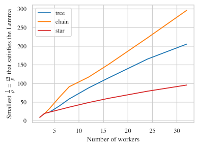
Figure 5: Optimal ratios for $\rho=p/m$ for Lemma 1 computed empirically for three common types of graph topologies.

Proof of key lemma 1.

First, let $\{\lambda_{i}\}$ and $\{\bm{v}_{i}\}$ be the eigenvalues and right eigenvectors of $\mathbf{W}$ where $\lambda_{1}=1$ and $\bm{v}_{1}=\mathbf{1}_{n(\tau_{\max}+1)}$, then

$$(\mathbf{W}-\mathbf{1}\bm{\pi}^{\top})\bm{v}_{1}= (\mathbf{W}-\mathbf{1}\bm{\pi}^{\top})\mathbf{1}=\mathbf{0}$$

$$(\mathbf{W}-\mathbf{1}\bm{\pi}^{\top})\bm{v}_{i}= \mathbf{W}\bm{v}_{i}-\mathbf{1}\bm{\pi}^{\top}\bm{v}_{i}=\mathbf{W}\bm{v}_{i}=\lambda_{i}\bm{v}_{i}\qquad\forall~{}i>1$$

where $\bm{\pi}^{\top}\bm{v}_{i}=0$ because

$$(1-\lambda_{i})\bm{\pi}^{\top}\bm{v}_{i}=\bm{\pi}^{\top}\bm{v}_{i}-\lambda_{i}\bm{\pi}^{\top}\bm{v}_{i}=(\bm{\pi}^{\top}\mathbf{W})\bm{v}_{i}-\bm{\pi}^{\top}(\mathbf{W}\bm{v}_{i})=0.$$

The spectrum of $\mathbf{W}-\mathbf{1}\bm{\pi}^{\top}$ are

$$\{0,\lambda_{2},\ldots,\lambda_{n(\tau_{\max}+1)}\},$$

and thus the spectral radius of $\mathbf{W}-\mathbf{1}\bm{\pi}^{\top}$ is $|\lambda_{2}|<1$. Since

$$\mathbf{W}^{m}-\mathbf{1}\bm{\pi}^{\top}=(\mathbf{W}-\mathbf{1}\bm{\pi}^{\top})^{m},$$

then $\mathbf{W}^{m}-\mathbf{1}\bm{\pi}^{\top}$ has a spectral radius of $|\lambda_{2}|^{m}<1$.

Then, we apply Gelfand’s formula (Lemma 7) with $\mathbf{A}=\mathbf{W}-\mathbf{1}\bm{\pi}^{\top}$ and can conclude that for a given $\varepsilon\in(0,1-|\lambda_{2}|)$, there exists a large enough integer $m>0$ such that

$$\|\mathbf{W}^{m}-\mathbf{1}\bm{\pi}^{\top}\|=\|(\mathbf{W}-\mathbf{1}\bm{\pi}^{\top})^{m}\|\leq(\rho(\mathbf{W}-\mathbf{1}\bm{\pi}^{\top})+\varepsilon)^{m}=(|\lambda_{2}|+\varepsilon)^{m}<1.$$

Thus

$$\|\mathbf{W}^{m}\mathbf{X}-\mathbf{1}\bm{\pi}^{\top}\mathbf{X}\|^{2}\leq\|\mathbf{W}^{m}-\mathbf{1}\bm{\pi}^{\top}\|^{2}\|\mathbf{X}-\mathbf{1}\bm{\pi}^{\top}\mathbf{X}\|^{2}\leq(1-p)^{2m}\|\mathbf{X}-\mathbf{1}\bm{\pi}^{\top}\mathbf{X}\|^{2}$$

where $p\in(0,1-|\lambda_{2}|)$. ∎

Definition G.

Given $\mathbf{W}$ and $m$, and $\tilde{\mathbf{I}}\in\mathbb{R}^{n(\tau_{\max}+1)\times n(\tau_{\max}+1)}$ is a matrix which satisfies

$$[\tilde{\mathbf{I}}]_{ij}=\begin{cases}1&i=j\leq n\\ 0&\text{Otherwise}.\end{cases}$$

We define constants $C_{1}^{2}:=\max_{i=0,\ldots,m-1}\|\mathbf{W}^{i}\tilde{\mathbf{I}}\|^{2}$ and $C=C(\mathbf{W})$ such that

$$C^{2}:=\frac{C_{1}^{2}}{\|\mathbf{W}^{\infty}\tilde{\mathbf{I}}\|^{2}}.$$

where $\mathbf{W}^{\infty}:=\mathbf{1}\bm{\pi}^{\top}$.

In addition, the $\|\mathbf{1}\bm{\pi}^{\top}\tilde{\mathbf{I}}\|^{2}$ can be computed as follows.

Lemma 8.

Given $\tilde{\mathbf{I}}$ in Definition G, we have the following estimate

$$\|\mathbf{1}\bm{\pi}^{\top}\tilde{\mathbf{I}}\|^{2}=n^{2}(\tau_{\max}+1)\pi_{0}^{2}\leq n^{3}\pi_{0}^{2}.$$

Proof.

For rank $r$ matrix $\|A\|^{2}\leq\|A\|_{F}^{2}\leq r\|A\|^{2}$. Since $\mathbf{1}\bm{\pi}^{\top}\tilde{\mathbf{I}}$ is a rank 1 matrix, we know that

$$\|\mathbf{1}\bm{\pi}^{\top}\tilde{\mathbf{I}}\|^{2}=\|\mathbf{1}\bm{\pi}^{\top}\tilde{\mathbf{I}}\|_{F}^{2}.$$

As the first n entries of $\bm{\pi}$ are $\pi_{0}$, we can compute that

$$\|\mathbf{1}\bm{\pi}^{\top}\tilde{\mathbf{I}}\|_{F}^{2}=n^{2}(\tau_{\max}+1)\pi_{0}^{2}.$$

∎

A.2.2 Useful inequalities and lemmas

For convex objective, the noise in B can be defined only at the minimizer $\mathbf{x}^{\star}$ which leads to H. This assumption is used in the proof of Proposition III.

Assumption H (Bounded noise at the optimum).

Let $\mathbf{x}^{\star}=\operatorname*{arg\,min}f(\mathbf{x})$ and define

$$\zeta_{i}^{2}:=\|\nabla f_{i}(\mathbf{x}^{\star})\|^{2},\qquad\bar{\zeta}^{2}:=\tfrac{1}{n}\textstyle\sum\nolimits_{i=1}^{n}\zeta_{i}^{2}.$$ (3)

Further, define

$$\sigma_{i}^{2}:=\operatorname{\mathbb{E}}_{\xi_{i}}\|\nabla F_{i}(\mathbf{x}^{\star},\xi_{i})-\nabla f_{i}(\mathbf{x}^{\star})\|^{2}$$

and similarly as above, $\bar{\sigma}^{2}:=\frac{1}{n}\sum_{i=1}^{n}\sigma_{i}^{2}$. We assume that $\bar{\sigma}^{2}$ and $\bar{\zeta}^{2}$ are bounded.

Lemma 9 (Cauchy-Schwartz inequality).

For arbitrary set of $n$ vectors $\{\mathbf{a}_{i}\}_{i=1}^{n}$, $a_{i}\in\mathbb{R}^{d}$

$$\left\|\sum_{i=1}^{n}\mathbf{a}_{i}\right\|^{2}\leq n\sum_{i=1}^{n}\|\mathbf{a}_{i}\|^{2}.$$ (4)

Lemma 10.

If function $g(\mathbf{x})$ is $L$-smooth, then

$$\|\nabla g(\mathbf{x})-\nabla g(\mathbf{y})\|^{2}\leq 2L(g(\mathbf{x})-g(\mathbf{y})-\langle\mathbf{x}-\mathbf{y},\nabla g(\mathbf{y})\rangle),\qquad\forall~{}\mathbf{x},\mathbf{y}\in\mathbb{R}^{d}.$$ (5)

Lemma 11.

Let $\mathbf{A}$ be a matrix with $\{\mathbf{a}_{i}\}_{i=1}^{n}$ as its columns and $\bar{\mathbf{a}}=\frac{1}{n}\sum_{i=1}^{n}\mathbf{a}_{i}$, $\bar{\mathbf{A}}=\bar{\mathbf{a}}\mathbf{1}^{\top}$ then

$$\|\mathbf{A}-\bar{\mathbf{A}}\|_{F}^{2}=\sum_{i=1}^{n}\|\mathbf{a}_{i}-\bar{\mathbf{a}}\|^{2}\leq\sum_{i=1}^{n}\|\mathbf{a}_{i}\|^{2}=\|\mathbf{A}\|^{2}_{F}.$$ (6)

Lemma 12.

Let $\mathbf{A}$,$\mathbf{B}$ be two matrices

$$\|\mathbf{A}\mathbf{B}\|_{F}^{2}\leq\|\mathbf{A}\|^{2}_{F}\|\mathbf{B}\|^{2}.$$ (7)

A.3 Results of Theorem I

In this subsection, we summarize the precise results of Theorem I for convex, strongly convex and non-convex cases. The complete proofs for each case are then given in the following Section A.4, Section A.5 and Section A.6.

Theorem’ I.

Given mixing matrix $\mathbf{W}$ and $\tilde{\mathbf{W}}$, constant $m$, $p$ defined in Lemma 1, $C$, $C_{1}$ defined in Definition G. Under Assumption A and B, then for any target accuracy $\varepsilon>0$,

Non-convex: if the objective is non-convex, then $\frac{1}{T+1}\sum_{t=0}^{T}\|\nabla f(\bar{\mathbf{x}}^{(t)})\|^{2}\leq\varepsilon$ after

$$\mathcal{O}\left(\frac{\bar{\sigma}^{2}}{n\varepsilon^{2}}+\frac{Cm\bar{\sigma}}{\sqrt{p}\varepsilon^{3/2}}+\frac{C_{1}m}{p\varepsilon}\right)Lr_{0}$$

iterations, where $r_{0}=f(\mathbf{x}^{(0)})-f^{\star}$.

Convex: if the objective is convex and $\mathbf{x}^{\star}$ is the minimizer, then $\tfrac{1}{T+1}\textstyle\sum\nolimits_{t=0}^{T}\left(f(\bar{\mathbf{x}}^{(t)})-f(\mathbf{x}^{\star})\right)\leq\varepsilon$ after

$$\mathcal{O}\left(\frac{\bar{\sigma}^{2}}{n\varepsilon^{2}}+\frac{Cm\sqrt{L}\bar{\sigma}}{\sqrt{p}\varepsilon^{3/2}}+\frac{Lm\sqrt{n}C}{p\varepsilon}\right)r_{0}$$

iterations, where $r_{0}=\|\mathbf{x}^{0}-\mathbf{x}^{\star}\|^{2}$.

Strongly-convex: if the objective is $\mu$ strongly convex and $\mathbf{x}^{\star}$ is the minimizer, then $\frac{1}{W_{T}}\sum_{t=0}^{T}w_{t}(\operatorname{\mathbb{E}}f(\bar{\mathbf{x}}^{(t)})-f^{\star})+\mu\operatorname{\mathbb{E}}\|\bar{\mathbf{x}}^{(T+1)}-\mathbf{x}^{\star}\|^{2}\leq\varepsilon$ after

$$\tilde{\mathcal{O}}\left(\frac{\bar{\sigma}^{2}}{\mu n\varepsilon^{2}}+\frac{Lm^{2}C^{2}\bar{\sigma}^{2}}{\mu np^{2}\varepsilon}+\frac{s}{a}\log{\frac{bsr_{0}}{\varepsilon}}\right)$$

iterations, where $r_{0}=\|\mathbf{x}^{0}-\mathbf{x}^{\star}\|^{2}$, $w_{t}=(1-\frac{\mu\gamma n\pi_{0}}{2})^{-(t+1)}$ and $W_{T}=\sum_{t=0}^{T}w_{t}$ and $a=\frac{\mu n\pi_{0}}{2}$, $b=\frac{2}{n\pi_{0}}$, $s=\frac{aT}{\ln\max\{\frac{ba^{2}T^{2}r_{0}}{\pi_{0}\bar{\sigma}^{2}},2\}}$.

In all three cases, the convergence rate is independent of the heterogeneity $\zeta^{2}$.

A.4 Proof of Theorem I in the convex case

Let $\bar{\mathbf{x}}^{(t)}:=\left(\bm{\pi}^{\top}\mathbf{Y}^{(t)}\right)^{\top}$ and $\bar{\mathbf{Y}}^{(t)}:=\mathbf{1}\bm{\pi}^{\top}\mathbf{Y}^{(t)}$. Let $\mathbf{x}^{\star}$ be the minimizer of $f$ and define the following iterates

• $r_{t}:=\|\bar{\mathbf{x}}^{(t)}-\mathbf{x}^{\star}\|^{2}$,

• $e_{t}:=f(\bar{\mathbf{x}}^{(t)})-f(\mathbf{x}^{\star})$,

• $\Xi_{t}:=\frac{1}{n}\|\bar{\mathbf{Y}}^{(t)}-\mathbf{Y}^{(t)}\|^{2}_{F}$.

The consensus distance $\Xi_{t}$ can be written as follows

$$\Xi_{t}=\frac{1}{n}\sum_{i=1}^{n}\sum_{\tau=0}^{\tau_{\max}}\|\bar{\mathbf{x}}^{(t)}-\mathbf{x}_{i}^{(t-\tau)}\|^{2}.$$ (8)

There is a related term $\sum_{i=1}^{n}\sum_{j=1}^{n}\|\bar{\mathbf{x}}^{(t)}-\mathbf{x}_{i}^{(t-\tau_{ij})}\|^{2}$ which will be used frequently in the proof. The next lemma explains their relations.

Lemma 13.

For all $t\geq 0$

$$\sum_{i=1}^{n}\sum_{j=1}^{n}\|\bar{\mathbf{x}}^{(t)}-\mathbf{x}_{i}^{(t-\tau_{ij})}\|^{2}\leq n^{2}\Xi_{t}.$$

where $\mathbf{x}^{(0)}=\mathbf{x}^{(-1)}=\ldots=\mathbf{x}^{(-\tau_{\max})}$.

Proof.

Rewrite the $\tau_{ij}$ as an indicator function

$$\sum_{i=1}^{n}\sum_{j=1}^{n}\|\bar{\mathbf{x}}^{(t)}-\mathbf{x}_{i}^{(t-\tau_{ij})}\|^{2}= \sum_{i=1}^{n}\sum_{j=1}^{n}\sum_{\tau=0}^{\tau_{\max}}\mathbf{1}_{\{\tau=\tau_{ij}\}}\|\bar{\mathbf{x}}^{(t)}-\mathbf{x}_{i}^{(t-\tau)}\|^{2}.$$

This term can be relaxed by removing the indicator function

$$\sum_{i=1}^{n}\sum_{j=1}^{n}\|\bar{\mathbf{x}}^{(t)}-\mathbf{x}_{i}^{(t-\tau_{ij})}\|^{2}\leq n\sum_{i=1}^{n}\sum_{\tau=0}^{\tau_{\max}}\|\bar{\mathbf{x}}^{(t)}-\mathbf{x}_{i}^{(t-\tau)}\|^{2}.$$

Then applying (8) for the consensus distance in vector form completes the proof. ∎

The next two propositions upper bound the difference between stochastic gradients and full gradients.

Proposition III.

Under A and B. Then for $t\geq 0$,

$$\operatorname{\mathbb{E}}\left\|\bm{\pi}^{\top}\tilde{\mathbf{W}}(\operatorname{\mathbb{E}}\mathbf{G}^{(t)}-\mathbf{G}^{(t)})\right\|^{2}\leq 3n\pi_{0}^{2}(L^{2}\Xi_{t}+2Le_{t}+\bar{\sigma}^{2}).$$

Proof.

Use $T_{0}$ to denote the left hand side quantity

$$T_{0} \hskip 11.38109pt:= \operatorname{\mathbb{E}}\left\|\bm{\pi}^{\top}\tilde{\mathbf{W}}(\operatorname{\mathbb{E}}\mathbf{G}^{(t)}-\mathbf{G}^{(t)})\right\|^{2}$$

$$\hskip 14.22636pt= \operatorname{\mathbb{E}}\left\|\frac{\pi_{0}}{n}\sum_{i=1}^{n}\sum_{j=1}^{n}(\nabla f_{j}(\mathbf{x}_{j}^{(t-\tau_{ij})})-\nabla F_{j}(\mathbf{x}_{j}^{(t-\tau_{ij})};\xi_{j}^{(t-\tau_{ij})}))\right\|^{2}$$

$$\stackrel{{\scriptstyle\text{Cauchy-Schwartz }\eqref{eq:cs}}}{{\leq}} \frac{\pi_{0}^{2}}{n}\sum_{i=1}^{n}\operatorname{\mathbb{E}}\left\|\sum_{j=1}^{n}(\nabla f_{j}(\mathbf{x}_{j}^{(t-\tau_{ij})})-\nabla F_{j}(\mathbf{x}_{j}^{(t-\tau_{ij})};\xi_{j}^{(t-\tau_{ij})}))\right\|^{2}.$$

Since the randomness inside the norm are independent, we have

$$T_{0}\leq \frac{\pi_{0}^{2}}{n}\sum_{i=1}^{n}\sum_{j=1}^{n}\operatorname{\mathbb{E}}\left\|\nabla f_{j}(\mathbf{x}_{j}^{(t-\tau_{ij})})-\nabla F_{j}(\mathbf{x}_{j}^{(t-\tau_{ij})};\xi_{j}^{(t-\tau_{ij})})\right\|^{2}.$$

Inside the vector norm, we can add and subtract terms the same terms and apply Cauchy-Schwartz (4)

$$T_{0}\leq \frac{3\pi_{0}^{2}}{n}\sum_{i=1}^{n}\sum_{j=1}^{n}\operatorname{\mathbb{E}}\big{\|}\nabla F_{j}(\mathbf{x}_{j}^{(t-\tau_{ij})};\xi_{j}^{(t-\tau_{ij})})-\nabla F_{j}(\bar{\mathbf{x}}^{(t)};\xi_{j}^{(t-\tau_{ij})})+\nabla f_{j}(\mathbf{x}_{j}^{(t-\tau_{ij})})-\nabla f_{j}(\bar{\mathbf{x}}^{(t)})\big{\|}^{2}$$

$$+\frac{3\pi_{0}^{2}}{n}\sum_{i=1}^{n}\sum_{j=1}^{n}\operatorname{\mathbb{E}}\left\|\nabla F_{j}(\bar{\mathbf{x}}^{(t)};\xi_{j}^{(t-\tau_{ij})})-\nabla F_{j}(\mathbf{x}^{\star};\xi_{j}^{(t-\tau_{ij})})+\nabla f_{j}(\bar{\mathbf{x}}^{(t)})-\nabla f_{j}(\mathbf{x}^{\star})\right\|^{2}$$

$$+\frac{3\pi_{0}^{2}}{n}\sum_{i=1}^{n}\sum_{j=1}^{n}\operatorname{\mathbb{E}}\left\|\nabla F_{j}(\mathbf{x}^{\star};\xi_{j}^{(t-\tau_{ij})}))-\nabla f_{j}(\mathbf{x}^{\star})\right\|^{2}.$$

Use the inequality that for $a=\operatorname{\mathbb{E}}Y$, $\operatorname{\mathbb{E}}\lVert Y-a\rVert^{2}=\operatorname{\mathbb{E}}\lVert Y\rVert^{2}-\lVert a\rVert^{2}\leq\operatorname{\mathbb{E}}\lVert Y\rVert^{2}$, then we have

$$T_{0}\leq \frac{3\pi_{0}^{2}}{n}\sum_{i=1}^{n}\sum_{j=1}^{n}\operatorname{\mathbb{E}}\big{\|}\nabla F_{j}(\mathbf{x}_{j}^{(t-\tau_{ij})};\xi_{j}^{(t-\tau_{ij})})-\nabla F_{j}(\bar{\mathbf{x}}^{(t)};\xi_{j}^{(t-\tau_{ij})})\big{\|}^{2}$$

$$+\frac{3\pi_{0}^{2}}{n}\sum_{i=1}^{n}\sum_{j=1}^{n}\operatorname{\mathbb{E}}\left\|\nabla F_{j}(\bar{\mathbf{x}}^{(t)};\xi_{j}^{(t-\tau_{ij})})-\nabla F_{j}(\mathbf{x}^{\star};\xi_{j}^{(t-\tau_{ij})})\right\|^{2}$$

$$+\frac{3\pi_{0}^{2}}{n}\sum_{i=1}^{n}\sum_{j=1}^{n}\operatorname{\mathbb{E}}\left\|\nabla F_{j}(\mathbf{x}^{\star};\xi_{j}^{(t-\tau_{ij})})-\nabla f_{j}(\mathbf{x}^{\star})\right\|^{2}$$

Applying A, Smoothness (5), and B (or H) to the three terms gives

$$T_{0}\leq \frac{3L^{2}\pi_{0}^{2}}{n}\sum_{i=1}^{n}\sum_{j=1}^{n}\big{\|}\mathbf{x}_{j}^{(t-\tau_{ij})}-\bar{\mathbf{x}}^{(t)}\big{\|}^{2}+6Ln\pi_{0}^{2}(f(\bar{\mathbf{x}}^{(t)})-f(\mathbf{x}^{\star}))+3\pi_{0}^{2}n\bar{\sigma}^{2}$$

$$\stackrel{{\scriptstyle\text{Lemma }\ref{lemma:Xi:alternative}}}{{\leq}} 3n\pi_{0}^{2}(L^{2}\Xi_{t}+2Le_{t}+\bar{\sigma}^{2}).$$

where in the last line we have used our previous Lemma 13. ∎

The next proposition is very similar to the Proposition III except that it considers the matrix form instead of the projection onto $\bm{\pi}$.

Proposition IV.

Under A and B. Then for $t\geq 0$,

$$\operatorname{\mathbb{E}}\left\|\tilde{\mathbf{W}}(\operatorname{\mathbb{E}}\mathbf{G}^{(t)}-\mathbf{G}^{(t)})\right\|^{2}_{F}\leq 3(L^{2}\Xi_{t}+2Le_{t}+\bar{\sigma}^{2}).$$

Proof.

$$\operatorname{\mathbb{E}}\left\|\tilde{\mathbf{W}}(\operatorname{\mathbb{E}}\mathbf{G}^{(t)}-\mathbf{G}^{(t)})\right\|_{F}^{2}$$

$$= \sum_{i=1}^{n}\operatorname{\mathbb{E}}\left\|\frac{1}{n}\sum_{j=1}^{n}(\nabla F(\mathbf{x}_{j}^{(t-\tau_{ij})};\xi_{j}^{(t-\tau_{ij})})-\nabla f_{j}(\mathbf{x}_{j}^{(t-\tau_{ij})}))\right\|^{2}$$

$$\leq \frac{1}{n^{2}}\sum_{i=1}^{n}\sum_{j=1}^{n}\operatorname{\mathbb{E}}\left\|\nabla F(\mathbf{x}_{j}^{(t-\tau_{ij})};\xi_{j}^{(t-\tau_{ij})})-\nabla f_{j}(\mathbf{x}_{j}^{(t-\tau_{ij})})\right\|^{2}$$

The rest of the proof is identical to the one of Proposition III. ∎

Lemma 14.

(Descent lemma for convex objective.) If $\gamma\leq\frac{1}{10Ln\pi_{0}}$, then

$$r_{t+1}\leq(1-\tfrac{\gamma\mu n\pi_{0}}{2})r_{t}-\gamma n\pi_{0}e_{t}+4\gamma Ln\pi_{0}\Xi_{t}+3\gamma^{2}n\pi_{0}^{2}\bar{\sigma}^{2}.$$

Proof.

Expand $r_{t+1}=\operatorname{\mathbb{E}}\|\bar{\mathbf{x}}^{(t+1)}-\mathbf{x}^{\star}\|^{2}$ as follows

$$\operatorname{\mathbb{E}}\|\bar{\mathbf{x}}^{(t+1)}-\mathbf{x}^{\star}\|^{2}= \operatorname{\mathbb{E}}\|\bar{\mathbf{x}}^{(t)}-\gamma\bm{\pi}^{\top}\tilde{\mathbf{W}}\mathbf{G}^{(t)}-\mathbf{x}^{\star}\|^{2}$$

$$= \operatorname{\mathbb{E}}\|\bar{\mathbf{x}}^{(t)}-\gamma\bm{\pi}^{\top}\tilde{\mathbf{W}}\operatorname{\mathbb{E}}\mathbf{G}^{(t)}-\mathbf{x}^{\star}+\gamma\bm{\pi}^{\top}\tilde{\mathbf{W}}(\operatorname{\mathbb{E}}\mathbf{G}^{(t)}-\mathbf{G}^{(t)})\|^{2}$$

Directly expand it into three terms

$$\operatorname{\mathbb{E}}\|\bar{\mathbf{x}}^{(t+1)}-\mathbf{x}^{\star}\|^{2}= \operatorname{\mathbb{E}}\left(\|\bar{\mathbf{x}}^{(t)}-\gamma\bm{\pi}^{\top}\tilde{\mathbf{W}}\operatorname{\mathbb{E}}\mathbf{G}^{(t)}-\mathbf{x}^{\star}\|^{2}+\gamma^{2}\|\bm{\pi}^{\top}\tilde{\mathbf{W}}(\operatorname{\mathbb{E}}\mathbf{G}^{(t)}-\mathbf{G}^{(t)}))\|^{2}\right.$$

$$+\left.\left\langle\bar{\mathbf{x}}^{(t)}-\gamma\bm{\pi}^{\top}\tilde{\mathbf{W}}\operatorname{\mathbb{E}}\mathbf{G}^{(t)}-\mathbf{x}^{\star},\gamma\bm{\pi}^{\top}\tilde{\mathbf{W}}(\operatorname{\mathbb{E}}\mathbf{G}^{(t)}-\mathbf{G}^{(t)}))\right\rangle\right)$$

where the 3rd term is 0 and the second term is bounded in Proposition III. The first term is independent of the randomness

$$\|\bar{\mathbf{x}}^{(t)}-\gamma\bm{\pi}^{\top}\tilde{\mathbf{W}}\operatorname{\mathbb{E}}\mathbf{G}^{(t)}-\mathbf{x}^{\star}\|^{2}$$

$$= \|\bar{\mathbf{x}}^{(t)}-\mathbf{x}^{\star}\|^{2}+\gamma^{2}\underbrace{\|\bm{\pi}^{\top}\tilde{\mathbf{W}}\operatorname{\mathbb{E}}\mathbf{G}^{(t)}\|^{2}}_{=:T_{1}}-2\gamma\underbrace{\langle\bm{\pi}^{\top}\tilde{\mathbf{W}}\operatorname{\mathbb{E}}\mathbf{G}^{(t)},\bar{\mathbf{x}}^{(t)}-\mathbf{x}^{\star}\rangle}_{=:T_{2}}.$$

Since $\bm{\pi}^{\top}\tilde{\mathbf{W}}\operatorname{\mathbb{E}}\mathbf{G}^{(t)}=\frac{\pi_{0}}{n}\sum_{i=1}^{n}\sum_{j=1}^{n}\nabla f_{i}(\mathbf{x}_{i}^{(t-\tau_{ij})})$, first bound $T_{1}$

$$T_{1} = \pi_{0}^{2}\left\|\frac{1}{n}\sum_{i=1}^{n}\sum_{j=1}^{n}\nabla f_{i}(\mathbf{x}_{i}^{(t-\tau_{ij})})\right\|^{2}$$

$$= \pi_{0}^{2}\left\|\frac{1}{n}\sum_{i=1}^{n}\sum_{j=1}^{n}(\nabla f_{i}(\mathbf{x}_{i}^{(t-\tau_{ij})})-\nabla f_{i}(\bar{\mathbf{x}}^{(t)})+\nabla f_{i}(\bar{\mathbf{x}}^{(t)})-\nabla f_{i}(\mathbf{x}^{\star}))\right\|^{2}$$

$$\leq 2\pi_{0}^{2}\left(\left\|\frac{1}{n}\sum_{i=1}^{n}\sum_{j=1}^{n}(\nabla f_{i}(\mathbf{x}_{i}^{(t-\tau_{ij})})-\nabla f_{i}(\bar{\mathbf{x}}^{(t)}))\right\|^{2}+\left\|\sum_{i=1}^{n}(\nabla f_{i}(\bar{\mathbf{x}}^{(t)})-\nabla f_{i}(\mathbf{x}^{\star}))\right\|^{2}\right)$$

$$\leq 2\pi_{0}^{2}L^{2}\sum_{i=1}^{n}\sum_{j=1}^{n}\left\|\mathbf{x}_{i}^{(t-\tau_{ij})}-\bar{\mathbf{x}}^{(t)}\right\|^{2}+2n\pi_{0}^{2}\sum_{i=1}^{n}\left\|\nabla f_{i}(\bar{\mathbf{x}}^{(t)})-\nabla f_{i}(\mathbf{x}^{\star})\right\|^{2}$$

$$\stackrel{{\scriptstyle\text{Smoothness }\eqref{eq:smooth:optimum}}}{{\leq}} 2\pi_{0}^{2}L^{2}\sum_{i=1}^{n}\sum_{j=1}^{n}\left\|\mathbf{x}_{i}^{(t-\tau_{ij})}-\bar{\mathbf{x}}^{(t)}\right\|^{2}+4Ln^{2}\pi_{0}^{2}(f(\bar{\mathbf{x}}^{(t)})-f(\mathbf{x}^{\star})),$$

Using again Lemma 13 we have

$$T_{1}\leq 2L^{2}n^{2}\pi_{0}^{2}\Xi_{t}+4Ln^{2}\pi^{2}_{0}e_{t}.$$

Then bound $T_{2}$

$$T_{2} = \frac{\pi_{0}}{n}\sum_{i=1}^{n}\sum_{j=1}^{n}\langle\nabla f_{i}(\mathbf{x}_{i}^{(t-\tau_{ij})}),\bar{\mathbf{x}}^{(t)}-\mathbf{x}^{\star}\rangle$$

$$= \frac{\pi_{0}}{n}\sum_{i=1}^{n}\sum_{j=1}^{n}(\langle\nabla f_{i}(\mathbf{x}_{i}^{(t-\tau_{ij})}),\bar{\mathbf{x}}^{(t)}-\mathbf{x}_{i}^{(t-\tau_{ij})}\rangle+\langle\nabla f_{i}(\mathbf{x}_{i}^{(t-\tau_{ij})}),\mathbf{x}_{i}^{(t-\tau_{ij})}-\mathbf{x}^{\star}\rangle)$$

$$\geq \frac{\pi_{0}}{n}\sum_{i=1}^{n}\sum_{j=1}^{n}(f_{i}(\bar{\mathbf{x}}^{(t)})-f_{i}(\mathbf{x}_{i}^{(t-\tau_{ij})})-\tfrac{L}{2}\|\bar{\mathbf{x}}^{(t)}-\mathbf{x}_{i}^{(t-\tau_{ij})}\|^{2}$$

$$+f_{i}(\mathbf{x}_{i}^{(t-\tau_{ij})})-f_{i}(\mathbf{x}^{\star})+\tfrac{\mu}{2}\|\mathbf{x}_{i}^{(t-\tau_{ij})}-\mathbf{x}^{\star}\|^{2})$$

$$= n\pi_{0}(f(\bar{\mathbf{x}}^{(t)})-f(\mathbf{x}^{\star}))+\frac{\pi_{0}}{n}\sum_{i=1}^{n}\sum_{j=1}^{n}(\tfrac{\mu}{2}\|\mathbf{x}_{i}^{(t-\tau_{ij})}-\mathbf{x}^{\star}\|^{2}-\tfrac{L}{2}\|\bar{\mathbf{x}}^{(t)}-\mathbf{x}_{i}^{(t-\tau_{ij})}\|^{2})$$

$$\geq n\pi_{0}(f(\bar{\mathbf{x}}^{(t)})-f(\mathbf{x}^{\star}))+\frac{\pi_{0}}{n}\sum_{i=1}^{n}\sum_{j=1}^{n}(\tfrac{\mu}{4}\|\bar{\mathbf{x}}^{(t)}-\mathbf{x}^{\star}\|^{2}-\tfrac{\mu+L}{2}\|\bar{\mathbf{x}}^{(t)}-\mathbf{x}_{i}^{(t-\tau_{ij})}\|^{2})$$

$$\stackrel{{\scriptstyle\text{Lemma }\ref{lemma:Xi:alternative}}}{{\geq}} n\pi_{0}e_{t}+\tfrac{n\mu\pi_{0}}{4}r_{t}-nL\pi_{0}\Xi_{t}$$

where the first inequality and the second inequality uses the $L$-smoothness and $\mu$-convexity of $f_{i}$.

Combine both $T_{1}$, $T_{2}$ and Proposition III we have

$$r_{t+1}\leq r_{t}+\gamma^{2}n^{2}\pi_{0}^{2}(2L^{2}\Xi_{t}+4Le_{t})-2\gamma n\pi_{0}(e_{t}+\tfrac{\mu}{4}r_{t}-L\Xi_{t})$$

$$+\gamma^{2}n(3L^{2}\pi_{0}^{2}\Xi_{t}+6L\pi_{0}^{2}e_{t}+3\pi_{0}^{2}\bar{\sigma}^{2})$$

$$= (1-\tfrac{\gamma\mu n\pi_{0}}{2})r_{t}-(2\gamma n\pi_{0}-4L\gamma^{2}n^{2}\pi_{0}^{2}-6L\gamma^{2}n\pi_{0}^{2})e_{t}$$

$$+(2\gamma^{2}L^{2}n^{2}\pi_{0}^{2}+2\gamma Ln\pi_{0}+3L^{2}\gamma^{2}n\pi_{0}^{2})\Xi_{t}+3\gamma^{2}n\pi_{0}^{2}\bar{\sigma}^{2}$$

In addition if $\gamma\leq\frac{1}{10Ln\pi_{0}}$, then we can simplify the coefficient of $e_{t}$ and $\Xi_{t}$

$$4L\gamma^{2}n^{2}\pi_{0}^{2}+6L\gamma^{2}n\pi_{0}^{2}\leq \gamma n\pi_{0}$$

$$2\gamma^{2}L^{2}n^{2}\pi_{0}^{2}+2\gamma Ln\pi_{0}+3L^{2}\gamma^{2}n\pi_{0}^{2}\leq 4\gamma Ln\pi_{0}$$

Then

$$r_{t+1}\leq(1-\tfrac{\gamma\mu n\pi_{0}}{2})r_{t}-\gamma n\pi_{0}e_{t}+4\gamma Ln\pi_{0}\Xi_{t}+3\gamma^{2}n\pi_{0}^{2}\bar{\sigma}^{2}.\qed$$

Lemma 15.

For $\gamma\leq\tfrac{p}{10LmC_{1}}$ we have

$$\frac{1}{T+1}\sum_{t=0}^{T}\Xi_{t}\leq C_{1}^{2}\gamma^{2}m^{2}\frac{24}{p}\frac{\bar{\sigma^{2}}}{n}+\frac{80Lm^{2}}{p^{2}}C_{1}^{2}\gamma^{2}\frac{1}{T+1}\sum_{t=0}^{T}e_{t}$$

where $C_{1}$ is defined in Definition G.

Proof.

First bound the consensus distance as follows:

$$n\Xi_{t}= \operatorname{\mathbb{E}}\|\mathbf{Y}^{(t)}-\bar{\mathbf{Y}}^{(t)}\|_{F}^{2}\leq\operatorname{\mathbb{E}}\|(\mathbf{Y}^{(t)}-\bar{\mathbf{Y}}^{(t-m)})-(\bar{\mathbf{Y}}^{(t)}-\bar{\mathbf{Y}}^{(t-m)})\|_{F}^{2}$$

$$\leq \operatorname{\mathbb{E}}\|\mathbf{Y}^{(t)}-\bar{\mathbf{Y}}^{(t-m)}\|_{F}^{2}$$

where the last inequality we use the simple matrix inequality (6). For $t\geq m$ unroll to $t-m$.

$$n\Xi_{t}\leq \operatorname{\mathbb{E}}\left\|\mathbf{W}^{m}\mathbf{Y}^{(t-m)}-\gamma\sum_{k=t-m}^{t-1}\mathbf{W}^{t-1-k}\tilde{\mathbf{W}}\mathbf{G}^{(k)}-\bar{\mathbf{Y}}^{(t-m)}\right\|_{F}^{2}$$

Separate the stochastic part and deterministic part.

$$n\Xi_{t}\leq \left\|\mathbf{W}^{m}\mathbf{Y}^{(t-m)}-\gamma\sum_{k=t-m}^{t-1}\mathbf{W}^{t-1-k}\tilde{\mathbf{W}}\operatorname{\mathbb{E}}\mathbf{G}^{(k)}-\bar{\mathbf{Y}}^{(t-m)}\right\|_{F}^{2}$$

$$+\operatorname{\mathbb{E}}\left\|\gamma\sum_{k=t-m}^{t-1}\mathbf{W}^{t-1-k}\tilde{\mathbf{W}}(\operatorname{\mathbb{E}}\mathbf{G}^{(k)}-\mathbf{G}^{(k)})\right\|_{F}^{2}$$

$$\leq \left\|\mathbf{W}^{m}\mathbf{Y}^{(t-m)}-\gamma\sum_{k=t-m}^{t-1}\mathbf{W}^{t-1-k}\tilde{\mathbf{W}}\operatorname{\mathbb{E}}\mathbf{G}^{(k)}-\bar{\mathbf{Y}}^{(t-m)}\right\|_{F}^{2}$$

$$+\gamma^{2}m\sum_{k=t-m}^{t-1}\operatorname{\mathbb{E}}\left\|\mathbf{W}^{t-1-k}\tilde{\mathbf{W}}(\operatorname{\mathbb{E}}\mathbf{G}^{(k)}-\mathbf{G}^{(k)})\right\|_{F}^{2}$$

Given $\tilde{\mathbf{I}}$ and $C_{1}$ in defined in Definition G, we know that $\tilde{\mathbf{W}}=\tilde{\mathbf{I}}\tilde{\mathbf{W}}$. Then use (7) and Proposition IV

$$n\Xi_{t}\leq \left\|\mathbf{W}^{m}\mathbf{Y}^{(t-m)}-\gamma\sum_{k=t-m}^{t-1}\mathbf{W}^{t-1-k}\tilde{\mathbf{W}}\operatorname{\mathbb{E}}\mathbf{G}^{(k)}-\bar{\mathbf{Y}}^{(t-m)}\right\|_{F}^{2}$$

$$+C_{1}^{2}\gamma^{2}m\sum_{k=t-m}^{t-1}\operatorname{\mathbb{E}}\left\|\tilde{\mathbf{W}}(\operatorname{\mathbb{E}}\mathbf{G}^{(k)}-\mathbf{G}^{(k)})\right\|_{F}^{2}$$

$$\leq \left\|\mathbf{W}^{m}\mathbf{Y}^{(t-m)}-\gamma\sum_{k=t-m}^{t-1}\mathbf{W}^{t-1-k}\tilde{\mathbf{W}}\operatorname{\mathbb{E}}\mathbf{G}^{(k)}-\bar{\mathbf{Y}}^{(t-m)}\right\|_{F}^{2}$$

$$+C_{1}^{2}\gamma^{2}m\sum_{k=t-m}^{t-1}3(L^{2}\Xi_{k}+2Le_{k}+\bar{\sigma}^{2})$$

Separate the first term as

$$n\Xi_{t}\leq (1+\alpha)\left\|\mathbf{W}^{m}\mathbf{Y}^{(t-m)}-\bar{\mathbf{Y}}^{(t-m)}\right\|_{F}^{2}+(1+\frac{1}{\alpha})\left\|\gamma\sum_{k=t-m}^{t-1}\mathbf{W}^{t-1-k}\tilde{\mathbf{W}}\operatorname{\mathbb{E}}\mathbf{G}^{(k)}\right\|_{F}^{2}$$

$$+C_{1}^{2}\gamma^{2}m\sum_{k=t-m}^{t-1}3(L^{2}\Xi_{k}+2Le_{k}+\bar{\sigma}^{2})$$

$$\leq (1+\alpha)(1-p)^{2m}\left\|\mathbf{Y}^{(t-m)}-\bar{\mathbf{Y}}^{(t-m)}\right\|_{F}^{2}+(1+\frac{1}{\alpha})\left\|\gamma\sum_{k=t-m}^{t-1}\mathbf{W}^{t-1-k}\tilde{\mathbf{W}}\operatorname{\mathbb{E}}\mathbf{G}^{(k)}\right\|_{F}^{2}$$

$$+C_{1}^{2}\gamma^{2}m\sum_{k=t-m}^{t-1}3(L^{2}\Xi_{k}+2Le_{k}+\bar{\sigma}^{2})$$

where the first inequality uses $(a+b)^{2}\leq(1+\varepsilon)a^{2}+(1+\frac{1}{\varepsilon})b^{2}$ and take $\varepsilon=(\frac{2-p}{2-2p})^{2m}-1$.

$$1+\tfrac{1}{\varepsilon}\leq 1+\tfrac{1-p}{mp}\leq 1+\tfrac{1}{mp}\leq\tfrac{2}{p}.$$

Then by applying our key lemma (Lemma 1) we have

$$n\Xi_{t}\ \leq\ \Big{(}1-\frac{p}{2}\Big{)}^{2m}\left\|\mathbf{Y}^{(t-m)}-\bar{\mathbf{Y}}^{(t-m)}\right\|_{F}^{2}+\frac{2m}{p}C_{1}^{2}\gamma^{2}\sum_{k=t-m}^{t-1}\left\|\tilde{\mathbf{W}}\operatorname{\mathbb{E}}\mathbf{G}^{(k)}\right\|_{F}^{2}$$

$$+C_{1}^{2}\gamma^{2}m\sum_{k=t-m}^{t-1}3(L^{2}\Xi_{k}+2Le_{k}+\bar{\sigma}^{2})$$

Next we bound $\operatorname{\mathbb{E}}\|\tilde{\mathbf{W}}\mathbf{G}^{(t^{\prime})}\|^{2}_{F}$,

$$\operatorname{\mathbb{E}}\|\tilde{\mathbf{W}}\operatorname{\mathbb{E}}\mathbf{G}^{(k)}\|^{2}_{F}= \textstyle\sum\nolimits_{i=1}^{n}\operatorname{\mathbb{E}}\|\tfrac{1}{n}\textstyle\sum\nolimits_{j=1}^{n}\nabla f_{j}(\mathbf{x}_{j}^{(k-\tau_{ij})})\|^{2}$$

$$= \textstyle\sum\nolimits_{i=1}^{n}\operatorname{\mathbb{E}}\|\tfrac{1}{n}\textstyle\sum\nolimits_{j=1}^{n}(\nabla f_{j}(\mathbf{x}_{j}^{(k-\tau_{ij})})-\nabla f_{j}(\bar{\mathbf{x}}^{(k)})+\nabla f_{j}(\bar{\mathbf{x}}^{(k)})-\nabla f_{j}(\mathbf{x}^{\star}))\|^{2}$$

$$\leq \tfrac{2}{n}\textstyle\sum\nolimits_{i=1}^{n}\textstyle\sum\nolimits_{j=1}^{n}(\|\nabla f_{j}(\mathbf{x}_{j}^{(k-\tau_{ij})})-\nabla f_{j}(\bar{\mathbf{x}}^{(k)})\|^{2}+\|\nabla f_{j}(\bar{\mathbf{x}}^{(k)})-\nabla f_{j}(\mathbf{x}^{\star}))\|^{2})$$

$$\leq \tfrac{2}{n}\textstyle\sum\nolimits_{i=1}^{n}\textstyle\sum\nolimits_{j=1}^{n}(L^{2}\|\mathbf{x}_{j}^{(k-\tau_{ij})}-\bar{\mathbf{x}}^{(k)}\|^{2}+\|\nabla f_{j}(\bar{\mathbf{x}}^{(k)})-\nabla f_{j}(\mathbf{x}^{\star}))\|^{2})$$

$$\stackrel{{\scriptstyle\text{Lemma }\ref{lemma:Xi:alternative}}}{{\leq}} 2L^{2}n\Xi_{k}+2\textstyle\sum\nolimits_{j=1}^{n}\|\nabla f_{j}(\bar{\mathbf{x}}^{(k)})-\nabla f_{j}(\mathbf{x}^{\star}))\|^{2}$$

$$\stackrel{{\scriptstyle\text{Smoothness }\eqref{eq:smooth:optimum}}}{{\leq}} 2L^{2}n\Xi_{k}+4nLe_{k}.$$

Then

$$n\Xi_{t}\leq (1-\frac{p}{2})^{2m}n\Xi_{t-m}+\frac{2m}{p}C_{1}^{2}\gamma^{2}\sum_{k=t-m}^{t-1}(2L^{2}n\Xi_{k}+4nLe_{k})+C_{1}^{2}\gamma^{2}m\sum_{k=t-m}^{t-1}3(L^{2}\Xi_{k}+2Le_{k}+\bar{\sigma}^{2})$$

Then

$$\Xi_{t}\leq (1-\frac{p}{2})^{2m}\Xi_{t-m}+\frac{2m}{p}C_{1}^{2}\gamma^{2}\sum_{k=t-m}^{t-1}(5L^{2}\Xi_{k}+10Le_{k})+3C_{1}^{2}\gamma^{2}m^{2}\frac{\bar{\sigma}^{2}}{n}.$$

Unroll for $t<m$.

We can apply similar steps

$$n\Xi_{t}\leq \operatorname{\mathbb{E}}\left\|\mathbf{W}^{(t)}\mathbf{Y}^{(0)}-\gamma\sum_{k=0}^{t-1}\mathbf{W}^{t-1-k}\tilde{\mathbf{W}}\mathbf{G}^{(k)}-\bar{\mathbf{Y}}^{(0)}\right\|_{F}^{2}=\operatorname{\mathbb{E}}\left\|\gamma\sum_{k=0}^{t-1}\mathbf{W}^{t-1-k}\tilde{\mathbf{W}}\mathbf{G}^{(k)}\right\|_{F}^{2}$$

$$\leq C_{1}^{2}\gamma^{2}m\sum_{k=0}^{t-1}\operatorname{\mathbb{E}}\left\|\tilde{\mathbf{W}}\mathbf{G}^{(k)}\right\|_{F}^{2}\leq 2C_{1}^{2}\gamma^{2}m\sum_{k=0}^{t-1}(5L^{2}n\Xi_{k}+10nLe_{k}+3\bar{\sigma}^{2})$$

Merge two parts together and sum over $t$.

$$\frac{1}{T+1}\sum_{t=0}^{T}\Xi_{t}\leq \left(1-\frac{p}{2}\right)^{2m}\frac{1}{T+1}\sum_{t=m}^{T}\Xi_{t-m}+6C_{1}^{2}\gamma^{2}m^{2}\frac{\bar{\sigma}^{2}}{n}$$

$$+\frac{2m}{p}C_{1}^{2}\gamma^{2}\frac{1}{T+1}\left(\sum_{t=m}^{T}\sum_{k=t-m}^{t-1}(5L^{2}\Xi_{k}+10Le_{k})+\sum_{t=0}^{m-1}\sum_{k=t-m}^{t-1}(5L^{2}\Xi_{k}+10Le_{k})\right)$$

$$\leq \left(1-\frac{p}{2}\right)^{2m}\frac{1}{T+1}\sum_{t=0}^{T}\Xi_{t}+6C_{1}^{2}\gamma^{2}m^{2}\frac{\bar{\sigma}^{2}}{n}+\frac{2m^{2}}{p}C_{1}^{2}\gamma^{2}\frac{1}{T+1}\sum_{t=0}^{T}\left(5L^{2}\Xi_{t}+10Le_{t}\right)$$

By taking $\gamma\leq\frac{p}{10CLm}$, then $\frac{10L^{2}m^{2}}{p}C_{1}^{2}\gamma^{2}\leq\frac{p}{4}$.

$$\frac{1}{T+1}\sum_{t=0}^{T}\Xi_{t}\leq C_{1}^{2}\gamma^{2}m^{2}\frac{24}{p}\frac{\bar{\sigma}^{2}}{n}+\frac{80Lm^{2}}{p^{2}}C_{1}^{2}\gamma^{2}\frac{1}{T+1}\sum_{t=0}^{T}e_{t}.\qed$$

Lemma 16 (Identical to [16, Lemma 15]).

For any parameters $r_{0}\geq 0,a\geq 0,b\geq 0,c\geq 0$ there exists constant stepsizes $\gamma\leq\frac{1}{c}$ such that

$$\Psi_{T}:=\frac{r_{0}}{\gamma(T+1)}+a\gamma+b\gamma^{2}\leq 2\left(\frac{ar_{0}}{T+1}\right)^{\tfrac{1}{2}}+2b^{\tfrac{1}{3}}\left(\frac{r_{0}}{T+1}\right)^{\tfrac{2}{3}}+\frac{cr_{0}}{T+1}.$$

Theorem V.

If $\gamma\leq\frac{p}{30LmC_{1}}$, then

$$\tfrac{1}{T+1}\textstyle\sum\nolimits_{t=0}^{T}\left(f(\bar{\mathbf{x}}^{(t)})-f(\mathbf{x}^{\star})\right)\leq 8\left(\frac{\bar{\sigma}^{2}r_{0}}{n(T+1)}\right)^{\tfrac{1}{2}}+2\left(\frac{16Cm\sqrt{L}\bar{\sigma}r_{0}}{\sqrt{p}(T+1)}\right)^{\tfrac{2}{3}}+\frac{30Lm\sqrt{n}Cr_{0}}{p(T+1)}.$$

where $r_{0}=\|\mathbf{x}^{0}-\mathbf{x}^{\star}\|^{2}$ and $C=C(\mathbf{W})$ is defined in Definition G.

Proof.

Reorganize Lemma 14 and average over time

$$\tfrac{1}{T+1}\textstyle\sum\nolimits_{t=0}^{T}e_{t}\leq\tfrac{1}{T+1}\textstyle\sum\nolimits_{t=0}^{T}\left(\tfrac{r_{t}}{\gamma n\pi_{0}}-\tfrac{r_{t+1}}{\gamma n\pi_{0}}\right)+\tfrac{4L}{T+1}\textstyle\sum\nolimits_{t=0}^{T}\Xi_{t}+3\gamma\pi_{0}\bar{\sigma}^{2}.$$

Combining with Lemma 15 gives

$$\tfrac{1}{T+1}\textstyle\sum\nolimits_{t=0}^{T}e_{t}\leq\tfrac{1}{T+1}\tfrac{r_{0}}{\gamma n\pi_{0}}+4L\left(C_{1}^{2}\gamma^{2}m^{2}\frac{24}{p}\frac{\bar{\sigma^{2}}}{n}+\frac{80Lm^{2}}{p^{2}}C_{1}^{2}\gamma^{2}\frac{1}{T+1}\sum_{t=0}^{T}e_{k}\right)+3\gamma\pi_{0}\bar{\sigma}^{2}$$

Select $\gamma\leq\frac{p}{30LmC_{1}}$ such that $\tfrac{320L^{2}}{p^{2}}\gamma^{2}m^{2}C_{1}^{2}\leq\frac{1}{2}$

$$\tfrac{1}{T+1}\textstyle\sum\nolimits_{t=0}^{T}e_{t}\leq\tfrac{2}{T+1}\tfrac{r_{0}}{\gamma n\pi_{0}}+6\gamma\pi_{0}\bar{\sigma}^{2}+\tfrac{96L}{p}\gamma^{2}m^{2}C_{1}^{2}\frac{\bar{\sigma}^{2}}{n}.$$

Applying Lemma 16 gives

$$\frac{1}{T+1}\sum_{t=0}^{T}e_{t}\leq 40\left(\frac{\bar{\sigma}^{2}r_{0}}{n(T+1)}\right)^{\tfrac{1}{2}}+2\left(\frac{\sqrt{mL}\bar{\sigma}r_{0}}{\sqrt{p}(T+1)}\frac{16C_{1}\sqrt{m}}{n\pi_{0}\sqrt{n}}\right)^{\tfrac{2}{3}}+\frac{dr_{0}}{n\pi_{0}(T+1)}$$

where $d=\max\{\frac{30LmC_{1}}{p},10Ln\pi_{0}\}=\frac{30LmC_{1}}{p}$. As in Lemma 8,

$$C_{1}=C\|\mathbf{1}\bm{\pi}^{\top}\tilde{\mathbf{I}}\|=Cn\sqrt{\tau_{\max}+1}\pi_{0}\leq Cn\sqrt{n}\pi_{0}.$$

We can further simplify it as

$$\frac{1}{T+1}\sum_{t=0}^{T}e_{t}\leq 40\left(\frac{\bar{\sigma}^{2}r_{0}}{n(T+1)}\right)^{\tfrac{1}{2}}+2\left(\frac{16Cm\sqrt{L}\bar{\sigma}r_{0}}{\sqrt{p}(T+1)}\right)^{\tfrac{2}{3}}+\frac{30Lm\sqrt{n}Cr_{0}}{p(T+1)}.\qed$$

A.5 Proof of Theorem I in the strongly convex case

The proof for strongly convex objective follows similar lines as [35]:

Theorem VI.

Let $a=\frac{\mu n\pi_{0}}{2}$, $b=\frac{2}{n\pi_{0}}$, $c=6\pi_{0}\bar{\sigma}^{2}$, $A=\frac{400L}{p^{2}}m^{2}C_{1}^{2}\bar{\sigma}^{2}$, and let $\gamma=\frac{1}{s}\leq\frac{1}{aT}\ln\max\{\frac{ba^{2}T^{2}r_{0}}{c},2\}$, then

$$\frac{1}{W_{T}}\sum_{t=0}^{T}w_{t}e_{t}+\mu r_{T+1}\leq \tilde{\mathcal{O}}\left(bsr_{0}\exp\left[-\frac{a(T+1)}{s}\right]+\frac{c}{a(T+1)}+\frac{A}{a^{2}(T+1)^{2}}\right)$$

where $w_{t}=(1-\frac{\mu\gamma n\pi_{0}}{2})^{-(t+1)}$.

Proof.

From Lemma 14 we know that if $\gamma\leq\frac{1}{10Ln\pi_{0}}$, then

$$r_{t+1}\leq(1-\tfrac{\gamma\mu n\pi_{0}}{2})r_{t}-\gamma n\pi_{0}e_{t}+4\gamma Ln\pi_{0}\Xi_{t}+3\gamma^{2}n\pi_{0}^{2}\bar{\sigma}^{2}.$$

Then

$$e_{t}\leq\frac{1}{\gamma n\pi_{0}}(1-\frac{\mu\gamma n\pi_{0}}{2})r_{t}-\frac{1}{\gamma n\pi_{0}}r_{t+1}+4L\Xi_{t}+3\gamma\pi_{0}\bar{\sigma}^{2}.$$

Multiply $w_{t}$ and sum over $t=0$ to $T$ and divided by $W_{T}$

$$\frac{1}{W_{T}}\sum_{t=0}^{T}w_{t}e_{t}\leq \frac{1}{W_{T}}\sum_{t=0}^{T}\left(\frac{1-\frac{\mu\gamma n\pi_{0}}{2}}{\gamma n\pi_{0}}w_{t}r_{t}-\frac{w_{t}}{\gamma n\pi_{0}}r_{t+1}\right)+\frac{4L}{W_{T}}\sum_{t=0}^{T}w_{t}\Xi_{t}+3\gamma\pi_{0}\bar{\sigma}^{2}.$$

Set $(1-\frac{\mu\gamma n\pi_{0}}{2})w_{t+1}=w_{t}$, then

$$\frac{1}{W_{T}}\sum_{t=0}^{T}w_{t}e_{t}\leq \frac{1}{W_{T}}\left(\frac{1-\frac{\mu\gamma n\pi_{0}}{2}}{\gamma n\pi_{0}}w_{0}r_{0}-\frac{1-\frac{\mu\gamma n\pi_{0}}{2}}{\gamma n\pi_{0}}w_{T+1}r_{T+1}\right)+\frac{4L}{W_{T}}\sum_{t=0}^{T}w_{t}\Xi_{t}+3\gamma\pi_{0}\bar{\sigma}^{2}.$$

Then using Lemma 15 we have

$$\frac{1}{W_{T}}\sum_{t=0}^{T}w_{t}e_{t}+\frac{1-\frac{\mu\gamma n\pi_{0}}{2}}{\gamma n\pi_{0}W_{T}}w_{T+1}r_{T+1}$$

$$\leq \frac{1}{W_{T}}\frac{1-\frac{\mu\gamma n\pi_{0}}{2}}{\gamma n\pi_{0}}w_{0}r_{0}+4L\left(\tfrac{80C_{1}^{2}Lm^{2}}{p^{2}}\gamma^{2}\tfrac{1}{W_{T}}\textstyle\sum\nolimits_{t^{\prime}=0}^{T}w_{t}\mathbf{e}_{t^{\prime}}+\tfrac{24}{p}\gamma^{2}m^{2}C_{1}^{2}\frac{\bar{\sigma}^{2}}{n}\right)+3\gamma\pi_{0}\bar{\sigma}^{2}$$

By taking $\gamma\leq\frac{p}{30LmC_{1}}$ we have $\frac{320L^{2}m^{2}C_{1}^{2}\gamma^{2}}{p^{2}}\leq\frac{1}{2}$, then

$$\frac{1}{W_{T}}\sum_{t=0}^{T}w_{t}e_{t}+\frac{1-\frac{\mu\gamma n\pi_{0}}{2}}{\gamma n\pi_{0}W_{T}}2w_{T+1}r_{T+1}\leq \frac{1}{W_{T}}\frac{1-\frac{\mu\gamma n\pi_{0}}{2}}{\gamma n\pi_{0}}2w_{0}r_{0}+6\gamma\pi_{0}\bar{\sigma}^{2}+\tfrac{400L}{p^{2}}\gamma^{2}m^{2}C_{1}^{2}\bar{\sigma}^{2}$$

Since $W_{T}\geq w_{T}=(1-\frac{\mu\gamma n\pi_{0}}{2})^{-(T+1)}$ and $W_{T}\leq\frac{2w_{T}}{\mu\gamma n\pi_{0}}$

$$\frac{1}{W_{T}}\sum_{t=0}^{T}w_{t}e_{t}+\mu r_{T+1}\leq \frac{(1-\frac{\mu\gamma n\pi_{0}}{2})^{T+1}}{\gamma n\pi_{0}}2w_{0}r_{0}+6\gamma\pi_{0}\bar{\sigma}^{2}+\tfrac{400L}{p^{2}}\gamma^{2}m^{2}C_{1}^{2}\bar{\sigma}^{2}$$

$$\leq \frac{e^{-\frac{\mu\gamma n\pi_{0}}{2}(T+1)}}{\gamma n\pi_{0}}2w_{0}r_{0}+6\gamma\pi_{0}\bar{\sigma}^{2}+\tfrac{400L}{p^{2}}\gamma^{2}m^{2}C_{1}^{2}\bar{\sigma}^{2}$$

Let $a=\frac{\mu n\pi_{0}}{2}$, $b=\frac{2}{n\pi_{0}}$, $c=6\pi_{0}\bar{\sigma}^{2}$, $A=\frac{400L}{p^{2}}m^{2}C_{1}^{2}\bar{\sigma}^{2}$, then

$$\frac{1}{W_{T}}\sum_{t=0}^{T}w_{t}e_{t}+\mu r_{T+1}\leq \frac{br_{0}}{\gamma}\exp[-a\gamma(T+1)]+c\gamma+A\gamma^{2}$$

Tuning stepsize.

Let $\gamma=\frac{1}{d}\leq\frac{1}{aT}\ln\max\{\frac{ba^{2}T^{2}r_{0}}{c},2\}$, then

$$\frac{1}{W_{T}}\sum_{t=0}^{T}w_{t}e_{t}+\mu r_{T+1}\leq \tilde{\mathcal{O}}\left(bsr_{0}\exp[-\frac{a(T+1)}{s}]+\frac{c}{a(T+1)}+\frac{A}{a^{2}(T+1)^{2}}\right).\qed$$

A.6 Proof of Theorem I in the non-convex case

Let $\bar{\mathbf{x}}^{(t)}:=\left(\bm{\pi}^{\top}\mathbf{Y}^{(t)}\right)^{\top}$ and $\bar{\mathbf{Y}}^{(t)}:=\mathbf{1}\bm{\pi}^{\top}\mathbf{Y}^{(t)}$. Let $f^{\star}$ be the optimal objective value at critical points. We can define the following iterates

1. $r_{t}:=\operatorname{\mathbb{E}}f(\bar{\mathbf{x}}^{(t)})-f^{\star}$ is the expected function suboptimality.

2. $e_{t}:=\|\nabla f(\bar{\mathbf{x}}^{(t)})\|^{2}$

3. $\Xi_{t}:=\frac{1}{n}\|\bar{\mathbf{Y}}^{(t)}-\mathbf{Y}^{(t)}\|^{2}_{F}$ is the consensus distance.

where the expectation is taken with respect to $\bm{\xi}^{(t)}\in\mathbb{R}^{n}$ the randomness across all workers at time $t$. Note that Lemma 13 still holds.

Proposition VII and Proposition VIII bound the stochastic noise of the gradient.

Proposition VII.

Under B, we have

$$\operatorname{\mathbb{E}}\lVert\bm{\pi}^{\top}\tilde{\mathbf{W}}(\mathbf{G}^{(t)}-\operatorname{\mathbb{E}}\mathbf{G}^{(t)})\rVert^{2}\leq n\pi_{0}^{2}\bar{\sigma}^{2}.$$ (9)

Proof.

Denote $\operatorname{\mathbb{E}}=\operatorname{\mathbb{E}}_{\bm{\xi}}$. Use Cauchy-Schwartz inequality Equation 4

$$\operatorname{\mathbb{E}}\lVert\bm{\pi}^{\top}\tilde{\mathbf{W}}(\mathbf{G}^{(t)}-\operatorname{\mathbb{E}}\mathbf{G}^{(t)})\rVert^{2}= \operatorname{\mathbb{E}}\left\|\frac{\pi_{0}}{n}\sum_{i=1}^{n}\sum_{j=1}^{n}(\nabla F_{j}(\mathbf{x}_{j}^{(t-\tau_{ij})};\xi_{j}^{(t-\tau_{ij})})-\nabla f_{j}(\mathbf{x}_{j}^{(t-\tau_{ij})}))\right\|^{2}$$

$$\leq \frac{\pi_{0}^{2}}{n}\sum_{i=1}^{n}\operatorname{\mathbb{E}}\left\|\sum_{j=1}^{n}\nabla F_{j}(\mathbf{x}_{j}^{(t-\tau_{ij})};\xi_{j}^{(t-\tau_{ij})})-\nabla f_{j}(\mathbf{x}_{j}^{(t-\tau_{ij})})\right\|^{2}$$

Now the randomness inside the norm are independent

$$\operatorname{\mathbb{E}}\lVert\bm{\pi}^{\top}\tilde{\mathbf{W}}(\mathbf{G}^{(t)}-\operatorname{\mathbb{E}}\mathbf{G}^{(t)})\rVert^{2}\operatorname{\mathbb{E}}\lVert\bm{\pi}^{\top}\tilde{\mathbf{W}}(\mathbf{G}^{(t)}-\operatorname{\mathbb{E}}\mathbf{G}^{(t)})\rVert^{2}\leq n\pi_{0}^{2}\bar{\sigma}^{2}.\qed$$

Proposition VIII.

Under B, we have

$$\operatorname{\mathbb{E}}\lVert\tilde{\mathbf{W}}(\mathbf{G}^{(t)}-\operatorname{\mathbb{E}}\mathbf{G}^{(t)})\rVert^{2}_{F}\leq\bar{\sigma}^{2}.$$ (10)

Next we establish the recursion of $r_{t}$

Lemma 17 (Descent lemma for non-convex case).

Under A and B. Let $\gamma\leq\frac{1}{8Ln\pi_{0}}$, then

$$r_{t+1}\leq r_{t}-\frac{\gamma n\pi_{0}}{4}e_{t}+2\gamma L^{2}n\pi_{0}\Xi_{t}+2\gamma^{2}Ln\pi^{2}_{0}\bar{\sigma}^{2}.$$

Proof.

Since $f$ is $L$-smooth,

$$\operatorname{\mathbb{E}}f(\bar{\mathbf{x}}^{(t+1)})= \operatorname{\mathbb{E}}f(\bar{\mathbf{x}}^{(t)}-\gamma\bm{\pi}^{\top}\tilde{\mathbf{W}}\mathbf{G}^{(t)})$$

$$\leq f(\bar{\mathbf{x}}^{(t)})-\gamma\underbrace{\langle\nabla f(\bar{\mathbf{x}}^{(t)}),\bm{\pi}^{\top}\tilde{\mathbf{W}}\operatorname{\mathbb{E}}\mathbf{G}^{(t)}\rangle}_{:=T_{1}}+\tfrac{\gamma^{2}L}{2}\underbrace{\operatorname{\mathbb{E}}\lVert\bm{\pi}^{\top}\tilde{\mathbf{W}}\mathbf{G}^{(t)}\rVert^{2}}_{:=T_{2}}$$

The first-order term $T_{1}$ has a lower bound

$$T_{1}= n\pi_{0}\langle\nabla f(\bar{\mathbf{x}}^{(t)}),\tfrac{1}{n\pi_{0}}\bm{\pi}^{\top}\tilde{\mathbf{W}}\operatorname{\mathbb{E}}\mathbf{G}^{(t)}\rangle$$

$$= n\pi_{0}\left(\lVert\nabla f(\bar{\mathbf{x}}^{(t)})\rVert^{2}+\langle\nabla f(\bar{\mathbf{x}}^{(t)}),\tfrac{1}{n\pi_{0}}\bm{\pi}^{\top}\tilde{\mathbf{W}}\operatorname{\mathbb{E}}\mathbf{G}^{(t)}-\nabla f(\bar{\mathbf{x}}^{(t)})\rangle\right)$$

$$\geq n\pi_{0}\left(\tfrac{1}{2}\lVert\nabla f(\bar{\mathbf{x}}^{(t)})\rVert^{2}-\tfrac{1}{2}\lVert\tfrac{1}{n\pi_{0}}\bm{\pi}^{\top}\tilde{\mathbf{W}}\operatorname{\mathbb{E}}\mathbf{G}^{(t)}-\nabla f(\bar{\mathbf{x}}^{(t)})\rVert^{2}\right)$$

$$= n\pi_{0}\left(\tfrac{1}{2}e_{t}-\tfrac{1}{2n^{4}}\lVert\textstyle\sum\nolimits_{i=1}^{n}\textstyle\sum\nolimits_{j=1}^{n}(\nabla f_{j}(\mathbf{x}_{j}^{(t-\tau_{ij})})-\nabla f_{j}(\bar{\mathbf{x}}^{(t)}))\rVert^{2}\right)$$

$$\geq n\pi_{0}\left(\tfrac{1}{2}e_{t}-\tfrac{L^{2}}{2n^{2}}\textstyle\sum\nolimits_{i=1}^{n}\textstyle\sum\nolimits_{j=1}^{n}\lVert\mathbf{x}_{j}^{(t-\tau_{ij})}-\bar{\mathbf{x}}^{(t)}\rVert^{2}\right)$$

$$\geq n\pi_{0}\left(\tfrac{1}{2}e_{t}-\tfrac{L^{2}}{2}\Xi_{t}\right)$$

as $a^{2}-\langle a,b\rangle\geq\frac{a^{2}}{2}-\frac{b^{2}}{2}$ for $a,b\geq 0$.

On the other hand, separate the stochastic part and deterministic part of $T_{2}$ we have

$$T_{2}\leq 2\operatorname{\mathbb{E}}\lVert\bm{\pi}^{\top}\tilde{\mathbf{W}}(\mathbf{G}^{(t)}-\operatorname{\mathbb{E}}\mathbf{G}^{(t)})\rVert^{2}+2\lVert\bm{\pi}^{\top}\tilde{\mathbf{W}}\operatorname{\mathbb{E}}\mathbf{G}^{(t)}\rVert^{2}.$$

Under B and Proposition VII, we know the first term

$$\operatorname{\mathbb{E}}\lVert\bm{\pi}^{\top}\tilde{\mathbf{W}}(\mathbf{G}^{(t)}-\operatorname{\mathbb{E}}\mathbf{G}^{(t)})\rVert^{2}\leq n\pi^{2}_{0}\bar{\sigma}^{2}.$$

Consider the second term

$$\lVert\bm{\pi}^{\top}\tilde{\mathbf{W}}\operatorname{\mathbb{E}}\mathbf{G}^{(t)}\rVert^{2}= \left\|\frac{\pi_{0}}{n}\sum_{i=1}^{n}\sum_{j=1}^{n}\nabla f_{j}(\mathbf{x}_{j}^{(t-\tau_{ij})})\right\|^{2}$$

$$= n^{2}\pi_{0}^{2}\left\|\frac{1}{n^{2}}\sum_{i=1}^{n}\sum_{j=1}^{n}\nabla f_{j}(\mathbf{x}_{j}^{(t-\tau_{ij})})-\nabla f(\bar{\mathbf{x}}^{(t)})+\nabla f(\bar{\mathbf{x}}^{(t)})\right\|^{2}$$

$$\leq 2n^{2}\pi_{0}^{2}\left\|\frac{1}{n^{2}}\sum_{i=1}^{n}\sum_{j=1}^{n}(\nabla f_{j}(\mathbf{x}_{j}^{(t-\tau_{ij})})-\nabla f_{j}(\bar{\mathbf{x}}^{(t)}))\right\|^{2}+2n^{2}\pi_{0}^{2}\left\|\nabla f(\bar{\mathbf{x}}^{(t)})\right\|^{2}$$

$$\leq 2\pi_{0}^{2}\sum_{i=1}^{n}\sum_{j=1}^{n}\left\|\nabla f_{j}(\mathbf{x}_{j}^{(t-\tau_{ij})})-\nabla f_{j}(\bar{\mathbf{x}}^{(t)})\right\|^{2}+2n^{2}\pi_{0}^{2}\left\|\nabla f(\bar{\mathbf{x}}^{(t)})\right\|^{2}$$

Combine B we have

$$\lVert\bm{\pi}^{\top}\tilde{\mathbf{W}}\operatorname{\mathbb{E}}\mathbf{G}^{(t)}\rVert^{2}\leq 2n^{2}\pi_{0}^{2}(L^{2}\Xi_{t}+e_{t}).$$

Therefore, the $T_{2}$ can be bounded as follows

$$T_{2}\leq 4n^{2}\pi^{2}_{0}(\tfrac{\bar{\sigma}^{2}}{n}+L^{2}\Xi_{t}+e_{t}).$$ (11)

Gathering everything together

$$r_{t+1}\leq r_{t}-\tfrac{\gamma n\pi_{0}}{2}(e_{t}-L^{2}\Xi_{t})+2\gamma^{2}Ln^{2}\pi^{2}_{0}(\tfrac{\bar{\sigma}^{2}}{n}+L^{2}\Xi_{t}+e_{t})$$

$$\leq r_{t}-\tfrac{\gamma n\pi_{0}}{2}(1-4\gamma Ln\pi_{0})e_{t}+\gamma L^{2}n\pi_{0}(1+2\gamma Ln\pi_{0})\Xi_{t}+2\gamma^{2}Ln\pi^{2}_{0}\bar{\sigma}^{2}$$

Let $\gamma\leq\frac{1}{8Ln\pi_{0}}$, then

$$r_{t+1}\leq r_{t}-\frac{\gamma n\pi_{0}}{4}e_{t}+2\gamma L^{2}n\pi_{0}\Xi_{t}+2\gamma^{2}Ln\pi^{2}_{0}\bar{\sigma}^{2}.\qed$$

Next we bound the consensus distance

Lemma 18 (Bounded consensus distance).

Under B,

$$\frac{1}{T+1}\sum_{t=0}^{T}\Xi_{t}\leq \frac{16C^{2}m^{2}}{p^{2}}\gamma^{2}\bar{\sigma}^{2}+\frac{16C^{2}m^{2}}{p^{2}}\gamma^{2}\frac{1}{T+1}\sum_{t=0}^{T}e_{k}\,.$$

Proof.

First bound the consensus distance by inserting $\bar{\mathbf{Y}}^{(t-m)}$

$$n\Xi_{t}= \operatorname{\mathbb{E}}\|\bar{\mathbf{Y}}^{(t)}-\mathbf{Y}^{(t)}\|^{2}_{F}\leq\operatorname{\mathbb{E}}\|(\bar{\mathbf{Y}}^{(t)}-\bar{\mathbf{Y}}^{(t-m)})-(\mathbf{Y}^{(t)}-\bar{\mathbf{Y}}^{(t-m)})\|^{2}_{F}$$

$$\leq \operatorname{\mathbb{E}}\|\mathbf{Y}^{(t)}-\bar{\mathbf{Y}}^{(t-m)}\|^{2}_{F}$$

where we used $\|A-\bar{A}\|_{F}^{2}=\sum_{i=1}^{n}\|\mathbf{a}_{i}-\bar{\mathbf{a}}\|^{2}\leq\sum_{i=1}^{n}\|\mathbf{a}_{i}\|^{2}=\|A\|^{2}_{F}$.

For $t\geq m$ unroll $\mathbf{Y}^{(t)}$ until $t-m$.

$$n\Xi_{t}\leq \operatorname{\mathbb{E}}\left\|\mathbf{W}^{m}\mathbf{Y}^{(t-m)}-\gamma\sum_{k=t-m}^{t-1}\mathbf{W}^{t-1-k}\tilde{\mathbf{W}}\mathbf{G}^{(k)}-\bar{\mathbf{Y}}^{(t-m)}\right\|^{2}_{F}$$

Separate stochastic part and deterministic part

$$n\Xi_{t}\leq \left\|\mathbf{W}^{m}\mathbf{Y}^{(t-m)}-\gamma\sum_{k=t-m}^{t-1}\mathbf{W}^{t-1-k}\tilde{\mathbf{W}}\operatorname{\mathbb{E}}\mathbf{G}^{(k)}-\bar{\mathbf{Y}}^{(t-m)}\right\|^{2}_{F}$$

$$+\operatorname{\mathbb{E}}\left\|\gamma\sum_{k=t-m}^{t-1}\mathbf{W}^{t-1-k}\tilde{\mathbf{W}}(\operatorname{\mathbb{E}}\mathbf{G}^{(k)}-\mathbf{G}^{(k)})\right\|^{2}_{F}$$

then let $C_{1}^{2}$ defined in Definition G and use $\|AB\|_{F}^{2}\leq\|A\|^{2}_{F}\|B\|^{2}$ and (10)

$$n\Xi_{t}\leq \left\|\mathbf{W}^{m}\mathbf{Y}^{(t-m)}-\gamma\sum_{k=t-m}^{t-1}\mathbf{W}^{t-1-k}\tilde{\mathbf{W}}\operatorname{\mathbb{E}}\mathbf{G}^{(k)}-\bar{\mathbf{Y}}^{(t-m)}\right\|^{2}_{F}$$

$$+C_{1}^{2}\gamma^{2}m\sum_{k=t-m}^{t-1}\operatorname{\mathbb{E}}\left\|\tilde{\mathbf{W}}(\operatorname{\mathbb{E}}\mathbf{G}^{(k)}-\mathbf{G}^{(k)})\right\|^{2}_{F}$$

$$\leq \left\|\mathbf{W}^{m}\mathbf{Y}^{(t-m)}-\gamma\sum_{k=t-m}^{t-1}\mathbf{W}^{t-1-k}\tilde{\mathbf{W}}\operatorname{\mathbb{E}}\mathbf{G}^{(k)}-\bar{\mathbf{Y}}^{(t-m)}\right\|^{2}_{F}+C_{1}^{2}\gamma^{2}m^{2}\bar{\sigma}^{2}$$

Apply Cauchy-Schwartz inequality with $\alpha>0$

$$n\Xi_{t}\leq (1+\alpha)\left\|\mathbf{W}^{m}\mathbf{Y}^{(t-m)}-\bar{\mathbf{Y}}^{(t-m)}\right\|^{2}_{F}+(1+\tfrac{1}{\alpha})\left\|\gamma\sum_{k=t-m}^{t-1}\mathbf{W}^{t-1-k}\tilde{\mathbf{W}}\operatorname{\mathbb{E}}\mathbf{G}^{(k)}\right\|^{2}_{F}+C_{1}^{2}\gamma^{2}m^{2}\bar{\sigma}^{2}$$

Applying Lemma 1 to the first term

$$n\Xi_{t}\leq (1+\alpha)(1-p)^{2m}\|\mathbf{Y}^{(t-m)}-\bar{\mathbf{Y}}^{(t-m)}\|_{F}^{2}+(1+\tfrac{1}{\alpha})\left\|\gamma\sum_{k=t-m}^{t-1}\mathbf{W}^{t-1-k}\tilde{\mathbf{W}}\operatorname{\mathbb{E}}\mathbf{G}^{(k)}\right\|^{2}_{F}+C_{1}^{2}\gamma^{2}m^{2}\bar{\sigma}^{2}$$

Take $\alpha=(\frac{2-p}{2-2p})^{2m}-1=(1+\frac{p}{2-2p})^{2m}-1\geq\frac{mp}{1-p}$ and use

$$1+\tfrac{1}{\alpha}\leq 1+\tfrac{1-p}{mp}\leq 1+\tfrac{1}{mp}\leq\tfrac{2}{p},$$

then use $\|AB\|_{F}^{2}\leq\|A\|^{2}_{F}\|B\|^{2}$

$$n\Xi_{t}\leq \left(1-\frac{p}{2}\right)^{2m}\|\mathbf{Y}^{(t-m)}-\bar{\mathbf{Y}}^{(t-m)}\|_{F}^{2}+\frac{2}{p}\left\|\gamma\sum_{k=t-m}^{t-1}\mathbf{W}^{t-1-k}\tilde{\mathbf{W}}\operatorname{\mathbb{E}}\mathbf{G}^{(k)}\right\|^{2}_{F}+C_{1}^{2}\gamma^{2}m^{2}\bar{\sigma}^{2}$$

$$\leq \left(1-\frac{p}{2}\right)^{2m}\|\mathbf{Y}^{(t-m)}-\bar{\mathbf{Y}}^{(t-m)}\|_{F}^{2}+\frac{2C_{1}^{2}m}{p}\gamma^{2}\sum_{k=t-m}^{t-1}\left\|\tilde{\mathbf{W}}\operatorname{\mathbb{E}}\mathbf{G}^{(k)}\right\|^{2}_{F}+C_{1}^{2}\gamma^{2}m^{2}\bar{\sigma}^{2}.$$

where the second term can be expanded by

$$\lVert\tilde{\mathbf{W}}\operatorname{\mathbb{E}}\mathbf{G}^{(k)}\rVert^{2}_{F}= \sum_{i=1}^{n}\left\|\frac{1}{n}\sum_{j=1}^{n}\nabla f_{j}(\mathbf{x}_{j}^{(k-\tau_{ij})})\right\|^{2}$$

$$= \sum_{i=1}^{n}\left\|\frac{1}{n}\sum_{j=1}^{n}\nabla f_{j}(\mathbf{x}_{j}^{(k-\tau_{ij})})-\nabla f(\bar{\mathbf{x}}^{(k)})+\nabla f(\bar{\mathbf{x}}^{(k)})\right\|^{2}$$

$$\leq 2\sum_{i=1}^{n}\left\|\frac{1}{n}\sum_{j=1}^{n}(\nabla f_{j}(\mathbf{x}_{j}^{(k-\tau_{ij})})-\nabla f_{j}(\bar{\mathbf{x}}^{(k)}))\right\|^{2}+2n\left\|\nabla f(\bar{\mathbf{x}}^{(k)})\right\|^{2}$$

$$\leq \frac{2}{n}\sum_{i=1}^{n}\sum_{j=1}^{n}\left\|\nabla f_{j}(\mathbf{x}_{j}^{(k-\tau_{ij})})-\nabla f_{j}(\bar{\mathbf{x}}^{(k)})\right\|^{2}+2n\left\|\nabla f(\bar{\mathbf{x}}^{(k)})\right\|^{2}$$

$$\leq 2nL^{2}\Xi_{k}+2ne_{k}$$

Combine and reduce the $n$ on both sides

$$\Xi_{t}\leq \left(1-\frac{p}{2}\right)^{2m}\Xi_{t-m}+2C_{1}^{2}m^{2}\gamma^{2}\frac{\bar{\sigma}^{2}}{n}+\frac{4C_{1}^{2}m}{p}\gamma^{2}\sum_{k=t-m}^{t-1}(L^{2}\Xi_{k}+e_{k}).$$

Unroll for $t<m$.

For $t<m$, we can apply similar steps

$$n\Xi_{t}\leq \operatorname{\mathbb{E}}\left\|\mathbf{W}^{(t)}\mathbf{Y}^{(0)}-\gamma\sum_{k=0}^{t-1}\mathbf{W}^{t-1-k}\tilde{\mathbf{W}}\mathbf{G}^{(k)}-\bar{\mathbf{Y}}^{(0)}\right\|^{2}_{F}=\operatorname{\mathbb{E}}\left\|\gamma\sum_{k=0}^{t-1}\mathbf{W}^{t-1-k}\tilde{\mathbf{W}}\mathbf{G}^{(k)}\right\|^{2}_{F}$$

$$\leq C_{1}^{2}\gamma^{2}m\sum_{k=0}^{t-1}\operatorname{\mathbb{E}}\left\|\tilde{\mathbf{W}}\mathbf{G}^{(k)}\right\|^{2}_{F}\leq 2C_{1}^{2}m\gamma^{2}\sum_{k=0}^{t-1}(\bar{\sigma}^{2}+nL^{2}\Xi_{k}+ne_{k}).$$

Finally, sum over $t$

$$\frac{1}{T+1}\sum_{t=0}^{T}\Xi_{t}\leq \left(1-\frac{p}{2}\right)^{2m}\frac{1}{T+1}\sum_{t=m}^{T}\Xi_{t-m}+2C_{1}^{2}m^{2}\gamma^{2}\frac{\bar{\sigma}^{2}}{n}$$

$$+\frac{4C_{1}^{2}m}{p}\gamma^{2}\frac{1}{T+1}\left(\sum_{t=m}^{T}\sum_{k=t-m}^{t-1}(L^{2}\Xi_{k}+e_{k})+\sum_{t=0}^{m-1}\sum_{k=0}^{t-1}(L^{2}\Xi_{k}+e_{k})\right)$$

$$\leq \left(1-\frac{p}{2}\right)^{2m}\frac{1}{T+1}\sum_{t=0}^{T}\Xi_{t}+2C_{1}^{2}m^{2}\gamma^{2}\frac{\bar{\sigma}^{2}}{n}+\frac{4C_{1}^{2}m^{2}}{p}\frac{\gamma^{2}}{T+1}\sum_{t=0}^{T}(L^{2}\Xi_{k}+e_{k}).$$

by taking $\gamma\leq\frac{p}{4CLm}$ we have $\frac{4C_{1}^{2}m^{2}}{p}\gamma^{2}L^{2}\leq\frac{p}{4}$, then rearrange the all of the $\Xi$ terms

$$\frac{1}{T+1}\sum_{t=0}^{T}\Xi_{t}\leq \frac{16C_{1}^{2}m^{2}}{p}\frac{\bar{\sigma}^{2}}{n}\gamma^{2}+\frac{16C_{1}^{2}m^{2}}{p^{2}}\gamma^{2}\frac{1}{T+1}\sum_{t=0}^{T}e_{k}\qed$$

We can use the lemmas for recursion and the descent in the consensus distance to conclude the following theorem.

Theorem IX.

Under A and B. For $\gamma\leq\frac{p}{16C_{1}Lm}$

$$\frac{1}{T+1}\sum_{t=0}^{T}\|\nabla f(\bar{\mathbf{x}}^{(t)})\|^{2}\leq 16\left(\frac{2L\bar{\sigma}^{2}r_{0}}{n(T+1)}\right)^{\frac{1}{2}}+2\left(\frac{16CLm\bar{\sigma}}{\sqrt{p}}\frac{8r_{0}}{T+1}\right)^{\frac{2}{3}}+\frac{16C_{1}Lm}{p}\frac{r_{0}}{T+1}$$

where $C=C(\mathbf{W})$ is defined in Definition G and $r_{0}=f(\mathbf{x}^{(0)})-f^{\star}$. Alternatively, for any target accuracy $\varepsilon$, $\frac{1}{T+1}\sum_{t=0}^{T}\|\nabla f(\bar{\mathbf{x}}^{(t)})\|^{2}\leq\varepsilon$ after

$$\mathcal{O}\left(\frac{\bar{\sigma}^{2}}{n\varepsilon^{2}}+\frac{Cm\bar{\sigma}}{\sqrt{p}\varepsilon^{3/2}}+\frac{C_{1}m}{p\varepsilon}\right)Lr_{0}$$

iterations.

Remark 19.

For gossip averaging [16], the rate with $\zeta^{2}=0$ is

$$\mathcal{O}\left(\frac{\bar{\sigma}^{2}}{n\varepsilon^{2}}+\frac{\sqrt{m}\bar{\sigma}}{\sqrt{p}\varepsilon^{3/2}}+\frac{m}{p\varepsilon}\right)Lr_{0}.$$

Proof.

From Lemma 17 we know that for $\gamma\leq\frac{1}{8Ln\pi_{0}}$

$$r_{t+1}\leq r_{t}-\frac{\gamma n\pi_{0}}{4}e_{t}+2\gamma L^{2}n\pi_{0}\Xi_{t}+2\gamma^{2}Ln\pi^{2}_{0}\bar{\sigma}^{2}.$$

Rearrange the terms and average over $t$

$$\frac{1}{T+1}\sum_{t=0}^{T}e_{t}\leq \frac{1}{T+1}\sum_{t=0}^{T}(\frac{4r_{t}}{\gamma n\pi_{0}}-\frac{4r_{t+1}}{\gamma n\pi_{0}})+\frac{8L^{2}}{T+1}\sum_{t=0}^{T}\Xi_{t}+8L\pi_{0}\gamma\bar{\sigma}^{2}$$

$$\leq \frac{1}{T+1}\frac{4r_{0}}{\gamma n\pi_{0}}+\frac{8L^{2}}{T+1}\sum_{t=0}^{T}\Xi_{t}+8L\pi_{0}\gamma\bar{\sigma}^{2}$$

On the other hand, from Lemma 18 for $\gamma\leq\frac{p}{4C_{1}Lm}$ we have

$$\frac{1}{T+1}\sum_{t=0}^{T}\Xi_{t}\leq \frac{16C_{1}^{2}m^{2}}{p}\frac{\bar{\sigma}^{2}}{n}\gamma^{2}+\frac{16C_{1}^{2}m^{2}}{p^{2}}\gamma^{2}\frac{1}{T+1}\sum_{t=0}^{T}e_{k}.$$

Then

$$\frac{1}{T+1}\sum_{t=0}^{T}e_{t}\leq \frac{1}{T+1}\frac{4r_{0}}{\gamma n\pi_{0}}+8L^{2}\frac{16C_{1}^{2}m^{2}}{p^{2}}\gamma^{2}\left(\frac{p\bar{\sigma}^{2}}{n}+\frac{1}{T+1}\sum_{t=0}^{T}e_{k}\right)+8L\pi_{0}\gamma\bar{\sigma}^{2}$$

By taking $\gamma\leq\frac{p}{16C_{1}Lm}$ such that $8L^{2}\frac{16C_{1}^{2}m^{2}}{p^{2}}\gamma^{2}\leq\frac{1}{2}$, then

$$\frac{1}{T+1}\sum_{t=0}^{T}e_{t}\leq \frac{1}{T+1}\frac{8r_{0}}{\gamma n\pi_{0}}+16L\pi_{0}\gamma\bar{\sigma}^{2}+\frac{16^{2}L^{2}C_{1}^{2}m^{2}}{np}\gamma^{2}\bar{\sigma}^{2}$$

Then applying Lemma 16 we have

$$\frac{1}{T+1}\sum_{t=0}^{T}e_{t}\leq 32\left(\frac{L\bar{\sigma}^{2}r_{0}}{n(T+1)}\right)^{\frac{1}{2}}+2\left(\frac{16C_{1}Lm\bar{\sigma}}{\sqrt{np}}\frac{8r_{0}}{n\pi_{0}(T+1)}\right)^{\frac{2}{3}}+\frac{dr_{0}}{T+1}$$

where $d=\max\{\frac{16C_{1}Lm}{p},8Ln\pi_{0}\}=\frac{16C_{1}Lm}{p}$. As in Lemma 8,

$$C_{1}=C\|\mathbf{1}\bm{\pi}^{\top}\tilde{\mathbf{I}}\|=Cn\sqrt{\tau_{\max}+1}\pi_{0}\leq Cn\sqrt{n}\pi_{0}.$$

We can further simplify it as

$$\frac{1}{T+1}\sum_{t=0}^{T}e_{t}\leq 32\left(\frac{L\bar{\sigma}^{2}r_{0}}{n(T+1)}\right)^{\frac{1}{2}}+2\left(\frac{16CLm\bar{\sigma}}{\sqrt{p}}\frac{8r_{0}}{T+1}\right)^{\frac{2}{3}}+\frac{dr_{0}}{T+1}.\qed$$

Appendix B Detailed experimental setup

B.1 Cifar-10

Table 6

Table 6: Default experimental settings for Cifar-10/VGG-11

Dataset	Cifar-10 [18]
Data augmentation	random horizontal flip and random $32\times 32$ cropping
Architecture	VGG-11 [17]
Training objective	cross entropy
Evaluation objective	top-1 accuracy
Number of workers	16
Topology	SGP: time-varying exponential, RelaySGD: double binary trees, baselines: best of ring or double binary trees
Gossip weights	Metropolis-Hastings (1/3 for ring)
Data distribution	Heterogeneous, not shuffled, according to Dirichlet sampling procedure from [20]
Batch size	32 patches per worker
Momentum	0.9 (Nesterov)
Learning rate	Tuned c.f. subsection C.1
LR decay	$/10$ at epoch 150 and 180
LR warmup	Step-wise linearly within 5 epochs, starting from 0
# Epochs	200
Weight decay	$10^{-4}$
Normalization scheme	no normalization layer
Repetitions	3, with varying seeds
Reported metric	Worst result of any worker of the worker’s mean test accuracy over the last 5 epochs

B.2 ImageNet

Table 7

Table 7: Default experimental settings for ImageNet

Dataset	ImageNet [5]
Data augmentation	random resized crop ($224\times 224$), random horizontal flip
Architecture	ResNet-20-EvoNorm [21, 20]
Training objective	cross entropy
Evaluation objective	top-1 accuracy
Number of workers	16
Topology	SGP: time-varying exponential, RelaySGD: double binary trees, baselines: best of ring or double binary trees
Gossip weights	Metropolis-Hastings (1/3 for ring)
Data distribution	Heterogeneous, not shuffled, according to Dirichlet sampling procedure from [20]
Batch size	32 patches per worker
Momentum	0.9 (Nesterov)
Learning rate	based on centralized training (scaled to $0.1\times\frac{32*16}{256}$)
LR decay	$/10$ at epoch $30,60,80$
LR warmup	Step-wise linearly within 5 epochs, starting from 0.1
# Epochs	90
Weight decay	$10^{-4}$
Normalization layer	EvoNorm [21]
Repetitions	Just one
Reported metric	Mean of all worker’s test accuracies over the last 5 epochs

B.3 BERT finetuning

Table 8

Table 8: Default experimental settings for BERT finetuning

Dataset	AG News [49]
Data augmentation	none
Architecture	DistilBERT [34]
Training objective	cross entropy
Evaluation objective	top-1 accuracy
Number of workers	16
Topology	restricted to a ring (chain for RelaySGD)
Gossip weights	Metropolis-Hastings (1/3 for ring)
Data distribution	Heterogeneous, not shuffled, according to Dirichlet sampling procedure from [20]
Batch size	32 patches per worker
Adam $\beta_{1}$	0.9
Adam $\beta_{2}$	0.999
Adam $\varepsilon$	$10^{-8}$
Learning rate	Tuned c.f. subsection C.3
LR decay	constant learning rate
LR warmup	no warmup
# Epochs	5
Weight decay	$0$
Normalization layer	LayerNorm [3]
Repetitions	3, with varying seeds
Reported metric	Mean of all worker’s test accuracies over the last 5 epochs

B.4 Random quadratics

We generate quadratics $\frac{1}{n}\sum_{i=1}^{n}f_{i}(\mathbf{x})$ of $\mathbf{x}\in\mathbb{R}^{d}$ where

$$f_{i}(\mathbf{x})=\lVert\mathbf{A}_{i}\mathbf{x}+\mathbf{b}_{i}\rVert^{2}_{2}.$$

Here the local Hessian $\mathbf{A}_{i}\in\mathbb{R}^{d\times d}$ control the shape of worker $i$’s local objective functions and the offset $\mathbf{b}_{i}\in\mathbb{R}^{d}$ allows for shifting the worker’s optimum. The generation procedure is as follows:

1. Sample $\mathbf{A}_{i}\in\mathbb{R}^{d\times d}$ from an i.i.d. element-wise standard normal distribution, independently for each worker.

2. Control the smoothness $L$ and strong-convexity constant $\mu$. Decompose $\mathbf{A}_{i}=\mathbf{U}_{i}\mathbf{S}_{i}\mathbf{V}_{i}^{\top}$ using Singular Value Decomposition, and replace $\mathbf{A}_{i}$ with $\mathbf{A}_{i}\leftarrow\mathbf{U}_{i}\tilde{\mathbf{S}}_{i}\mathbf{V}_{i}^{\top}$, where $\tilde{\mathbf{S}}_{i}\in\mathbb{R}^{d\times d}$ is a diagonal matrix with diagonal entries $[\mu,\frac{d-2}{d-1}\mu+\frac{1}{d-1}L,\ldots,L]$.

3. Control the heterogeneity $\zeta_{2}$ by shifting worker’s optima into random directions.

   1. Sample random directions $\mathbf{d}_{i}\in\mathbb{R}^{d}$ from an i.i.d. element-wise standard normal distributions, independently for each worker.

   2. Instantiate a scalar $s\leftarrow 1$ and optimize it using binary search:

   3. Move local optima by $s\mathbf{d}_{i}$ by setting $\mathbf{b}_{i}\leftarrow\mathbf{A}_{i}s\mathbf{d}_{i}$.

   4. Move all optima $\mathbf{b}_{i}\leftarrow\mathbf{b}_{i}-\mathbf{A}_{i}\mathbf{x}^{\star}$ such that the global optimum $\mathbf{x}^{\star}$ remains at zero.

   5. Evaluate $\zeta^{2}=\frac{1}{n}\sum_{i=1}^{n}\lVert\nabla f_{i}(\mathbf{x}^{\star})\rVert^{2}_{2}$ and adjust the scale factor $s$ until $\zeta^{2}$ is as desired. Repeat from step (c).

4. Control the initial distance to the optimum $r_{0}$. Sample a random vector for the optimum $\mathbf{x}^{\star}$ from an i.i.d. element-wise normal distribution and scale it to have norm $r_{0}$. Shift all worker’s optima in this direction by updating $\mathbf{b}_{i}\leftarrow\mathbf{b}_{i}+\mathbf{A}_{i}\mathbf{x}^{\star}$.

Appendix C Hyper-parameters and tuning details

C.1 Cifar-10

For our image classification experiments on Cifar-10, we have independently tuned learning rates for each algorithm, at each data heterogeneity level $\alpha$, and separately for SGD with and without momentum. We followed the following procedure:

1. We found an appropriate learning rate for centralized (all-reduce) training (by using the procedure below)

2. Start the search from this learning rate. For RelaySGD, we apply a correction computed as in subsection D.1.

3. Grid-search the learning rate by multiplying and dividing by powers of two. Try larger and smaller learning rates, until the best result found so far is sandwiched between two learning rates that gave worse results.

4. Repeat the experiment with 3 random seeds.

5. If any of those replicas diverged, reduce the learning rate by a factor two until it does.

For the experiments in Table 1, we used the learning rates listed in Table 9.

Table 9: Learning rates used for Cifar-10/ VGG-11. Numbers between parentheses indicate the number of converged replications with this learning rate.

Algorithm	Topology	$\alpha=1.00$	$\alpha=0.1$	$\alpha=.01$
		(most homogeneous)		(most heterogeneous)
All-reduce	fully connected	0.100 (3)	0.100 (3)	0.100 (3)
$\quad+$momentum		0.100 (3)	0.100 (3)	0.100 (3)
RelaySGD	binary trees	1.200 (3)	0.600 (3)	0.300 (3)
$\quad+$local momentum		0.600 (3)	0.300 (3)	0.150 (3)
DP-SGD [19]	ring	0.400 (3)	0.100 (3)	0.200 (3)
$\quad+$quasi-global mom. [20]		0.100 (3)	0.025 (3)	0.050 (3)
D2 [36]	ring	0.200 (3)	0.200 (3)	0.100 (3)
$\quad+$local momentum		0.050 (3)	0.050 (3)	0.013 (3)
Stochastic gradient push [2]	time-varying exponential [2]	0.400 (3)	0.200 (3)	0.200 (3)
$\quad+$local momentum		0.100 (3)	0.100 (3)	0.025 (3)

C.2 ImageNet

Due to the high resource requirements, we did not tune the learning rate for our ImageNet experiments. We identified a suitable learning rate based on prior work, and used this for all experiments. For RelaySGD, we used the analytically computed learning rate correction from subsection D.1.

C.3 BERT finetuning

For DistilBERT fine-tuning experiments on AG News, we have independently tuned learning rate for each algorithm. We search the learning rate in the grid of $\{1e-5,3e-5,5e-5,7e-5,9e-5\}$ and we extend the grid to ensure that the best hyper-parameter lies in the middle of our search grids, otherwise we extend our search grid.

For the experiments in Table 4, we used the learning rates listed in Table 10.

Table 10: Tuned learning rates used for AG News / DistilBERT (Table 4)

Algorithm	Topology	Learning rate
Centralized Adam	fully-connected	3e-5
Relay-Adam	chain	9e-4
DP-SGD Adam	ring	1e-6
Quasi-global Adam [20]	ring	1e-6

C.4 Random quadratics

For Figures 2 and 3, we tuned the learning rate for each compared method to reach a desired quality level as quickly as possible, using binary search. We made a distinction between methods that are expected to converge linearly, and methods that are expected to reach a plateau. For experiments with stochastic noise, we tuned a learning rate without noise first, and then lowered the learning rate if needed to reach a desirable plateau. Please see the supplied code for implementation details.

Appendix D Algorithmic details

D.1 Learning-rate correction for RelaySGD

In DP-SGD as well as all other algorithms we compared to, a gradient-based update $\mathbf{u}^{(t)}_{i}$ from worker $i$ at time $t$ will eventually, as $t\to\infty$ distribute uniformly with weights $\frac{1}{n}$ over all workers. In RelaySGD, the update also distributes uniformly (typically much quicker), but it will converge to a weight $\alpha\leq\frac{1}{n}$. The constant $\alpha$ is fixed throughout training and depends only on the network topology used. To correct for this loss in energy, you can scale the learning rate by a factor $\frac{1}{\alpha n}$.

Experimentally, we pre-compute $\alpha$ for each architecture by initialing a scalar model for each worker to zero, updating the models to $1$, and running RelaySGD until convergence with no further model updates. The worker will converge to the value $\alpha$. The correction factors that result from this procedure are illustrated in Figure 6.

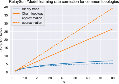
Figure 6: This network-topology-dependent correction factor is computed as follows: Each worker initializes a scalar model to 0 and sends a single fixed value 1 as gradient update through the RelaySGD algorithm. For DP-SGD and all-reduce, workers would converge to 1, but for RelaySGD, we lose some of this energy. If the workers converge to a value $\alpha$, we will scale the learning rate with $1/\alpha$ for RelaySGD compared to all-reduce.

In our deep learning experiments, we find that for each learning rate were centralized SGD converges, RelaySGD with the corrected learning rate converges too. Note that this learning rate correction is only useful if you already have a tuned learning rate from centralized experiments, or experiments with algorithms such as DP-SGD. If you start from scratch, tuning the learning rate for RelaySGD is no different form tuning the learning rate for any of the other algorithms.

D.2 RelaySGD with momentum

RelaySGD follows Algorithm 1, but replaces the local update in line 3 with a local momentum. For Nesterov momentum with momentum-parameter $\alpha$, this is:

$$\mathbf{m}_{i}^{(t)} =\alpha\,\mathbf{m}_{i}^{(t-1)}+\nabla f_{i}(\mathbf{x}_{i}^{(t)})\quad\color[rgb]{.5,.5,.5}(\text{initialize }\mathbf{m}_{i}^{0}=0)$$

$$\mathbf{x}_{i}^{(t+\nicefrac{{1}}{{2}})} =\mathbf{x}_{i}^{(t)}-\gamma\left(\nabla f_{i}(\mathbf{x}_{i}^{(t)})+\alpha\,\mathbf{m}_{i}^{(t)}\right).$$

D.3 RelaySGD with Adam

Modifiying RelaySGD (Algorithm 1) to use Adam is analogous to RelaySGD with momentum (subsection D.2). All Adam state is updated locally. We use the standard Adam implementation of PyTorch 1.18.

D.4 D² with momentum

We made slight modifications to the D² algorithm from Tang et al. [36] to allow time-varying learning rates and local momentum. The version we use is listed as Algorithm 2. Note that D² requires the smallest eigenvalue of the gossip matrix $\mathbf{W}$ to be $\geq-1/3$. This property is satisfied for Metropolis-Hasting matrices used on rings and double binary trees, but it was not in our Social Network Graph experiment (Figure 3). For this reason, we used the gossip matrix $(\mathbf{W}+\mathbf{I})/2$, from the otherwise-equivalent Exact Diffusion algorithm [45] on the social network graph.

Algorithm 2 D² [36] with momentum

1:$\forall~{}i,~{}\mathbf{x}_{i}^{(0)}=\mathbf{x}^{(0)}$, learning rate $\gamma$, momentum $\alpha$, gossip matrix $\mathbf{W}\in\mathbb{R}^{n\times n}$, $\mathbf{c}_{i}^{(0)}=\mathbf{0}\in\mathbb{R}^{d}$.

2:for $t=0,1,\ldots$ do

3:     for node $i$ in parallel

4:         Update the local momentum buffer $\mathbf{m}_{i}^{(t)}=\alpha\,\mathbf{m}_{i}^{(t-1)}+\nabla f_{i}(\mathbf{x}_{i}^{(t)})$.

5:         Compute a local update $\mathbf{u}_{i}^{(t)}=-\gamma(\nabla f_{i}(\mathbf{x}_{i}^{(t)})+\alpha\,\mathbf{m}_{i}^{(t)})$.

6:         Update the local model $\mathbf{x}^{(t+\nicefrac{{1}}{{2}})}_{i}=\mathbf{x}^{(t)}_{i}+\mathbf{u}_{i}^{(t)}+\mathbf{c}_{i}^{(t)}$.

7:         Average with neighbors: $\mathbf{x}^{(t+1)}_{i}=\sum_{j\in\mathcal{N}_{i}}\mathbf{W}_{ij}\mathbf{x}_{j}^{(t+\nicefrac{{1}}{{2}})}$.

8:         Update the local correction $\mathbf{c}^{(t+1)}_{i}=\mathbf{x}^{(t+1)}_{i}-\mathbf{x}^{(t)}_{i}-\mathbf{u}_{i}^{(t)}$.

9:     end for

10:end for

D.5 Gradient Tracking

Algorithm 3 lists our implementation of Gradient Tracking from Lorenzo and Scutari [22].

Algorithm 3 Gradient Tracking [22]

1:$\forall~{}i,~{}\mathbf{x}_{i}^{(0)}=\mathbf{x}^{(0)}$, learning rate $\gamma$, gossip matrix $\mathbf{W}\in\mathbb{R}^{n\times n}$, $\mathbf{c}_{i}^{(0)}=\mathbf{0}\in\mathbb{R}^{d}$.

2:for $t=0,1,\ldots$ do

3:     for node $i$ in parallel

4:         Compute a local update $\mathbf{u}_{i}^{(t)}=-\gamma\nabla f_{i}(\mathbf{x}_{i}^{(t)})$.

5:         Update the local model $\mathbf{x}^{(t+\nicefrac{{1}}{{2}})}_{i}=\mathbf{x}^{(t)}_{i}+\mathbf{u}_{i}^{(t)}+\mathbf{c}_{i}^{(t)}$.

6:         Average with neighbors: $\mathbf{x}^{(t+1)}_{i}=\sum_{j\in\mathcal{N}_{i}}\mathbf{W}_{ij}\mathbf{x}_{j}^{(t+\nicefrac{{1}}{{2}})}$.

7:         Update the correction and average: $\mathbf{c}^{(t+1)}_{i}=\sum_{j\in\mathcal{N}_{i}}\mathbf{W}_{ij}\left(\mathbf{c}_{i}^{(t)}-\mathbf{u}_{i}^{(t)}\right)$.

8:     end for

9:end for

D.6 Stochastic Gradient Push with the time-varying exponential topology

Stochastic Gradient Push with the time-varying exponential topology from [2] demonstrates that decentralized learning algorithms can reduce communication in a data center setting where each node could talk to each other node. Algorithm 4 lists our implementation of this algorithm.

Algorithm 4 Stochastic Gradient Push with time-varying exponential topology [2]

1:$\forall~{}i,~{}\mathbf{x}_{i}^{(0)}=\mathbf{x}^{(0)}$, learning rate $\gamma$, $n=2^{k}$ workers, $t^{\prime}=0$.

2:for $t=0,1,\ldots$ do

3:     for node $i$ in parallel

4:         $\mathbf{x}^{(t+\nicefrac{{1}}{{2}})}_{i}=\mathbf{x}^{(t)}_{i}+\mathbf{u}_{i}^{(t)}{\color[rgb]{0.121,0.466,0.705}-\gamma\nabla f_{i}(\mathbf{x}_{i}^{(t)})}$.(or momentum/Adam, like RelaySGD)

5:         for 2 communication steps to equalize bandwidth with RelaySGD do

6:              Compute an offset $o$ = $2^{t^{\prime}\text{ mod }k}$.

7:              Send $\mathbf{x}^{(t+\nicefrac{{1}}{{2}})}_{i}$ to worker $i-o$.

8:              Receive and overwrite $\mathbf{x}_{i}^{(t+\nicefrac{{1}}{{2}})}\leftarrow\frac{1}{2}\left(\mathbf{x}^{(t+\nicefrac{{1}}{{2}})}_{i}+\mathbf{x}^{(t+\nicefrac{{1}}{{2}})}_{i+o}\right)$.

9:              $t^{\prime}\leftarrow t^{\prime}+1$.

10:         end for

11:         Set $\mathbf{x}_{i}^{(t+1)}=\mathbf{x}_{i}^{(t+\nicefrac{{1}}{{2}})}$.

12:     end for

13:end for

Appendix E Additional experiments on RelaySGD

E.1 Rings vs double binary trees on Cifar-10

In our experiments that target data-center inspired scenarios where the network topology is arbitrarily selected by the user to save bandwidth, RelaySGD uses double binary trees to communicate. They use the same memory and bandwidth as rings (2 models sent/received per iteration) but they delays only scale with $\log n$, enabling RelaySGD, in theory, to run with very large numbers of workers $n$. Table 11 shows that in our Cifar-10 experiments with 16 there are minor improvements from using double binary trees over rings. Our baselines DP-SGD and D², however, perform significantly better on rings than on trees, so we use those results in the main paper.

Table 11: Comparing the performance of the algorithms in Table 1 on rings and double binary trees in the high-heterogeneity setting $\alpha=0.01$. In both topologies, workers send and receive two full models per update step. With 16 workers, RelaySGD with momentum seems to benefit from double binary trees, RelaySGD has more consistently good results on a chain. We still opt for double binary trees based on their promise to scale to many workers. Other methods do not benefit from double binary trees over rings.

Algorithm	Ring (Chain for RelaySGD)	Double binary trees
RelaySGD	86.5%	84.6%
$\quad+$local momentum	88.4%	89.1%
DP-SGD [19]	53.9%	36.0%
$\quad+$quasi-global mom. [20]	63.3%	57.5%
D2 [36]	38.2%	did not converge
$\quad+$local momentum	61.0%	did not converge

E.2 Scaling the number of workers on Cifar-10

In this experiment (Table 12), use momentum-SGD on 16, 32 and 64 workers compare the scaling of RelaySGD to SGP [2]. We fix the parameter $\alpha$ that determines the level of data heterogeneity to $\alpha=0.01$. Note that this level of $\alpha$ could lead to more challenging heterogeneity when there are many workers (and hence many smaller local subsets of the data), compared to when there are few workers.

Table 12: Scaling the number of workers in heterogeneous Cifar-10. The heterogeneity level $\alpha=0.01$ is kept constant, although it does change its meaning when the number of workers changes. RelaySGD scales at least well as Stochastic Gradient Push [2] (with equal communication budget). It is surprising that RelaySGD with 64 workers performs significantly better on a chain topology than on the double binary trees. This behavior does not match what our observations on quadratic toy-problems.

Algorithm	Topology	16 workers	32 workers	64 workers
All-reduce (baseline)	fully connected	89.5%	88.9%	87.2%
RelaySGD	binary trees	89.3%	86.1%	63.7%
	chain	88.4%	86.6%	83.1%
Stochastic gradient push [2]	time-varying exponential [2]	87.0%	68.9%	62.4%

Table 13: Tuned learning rates for Table 12. We tuned the learning rate for each setting on a multiplicative grid with spacing $\sqrt{2}$, and then repeated each experiment 3 times. If both repetitions diverged, we would change to a smaller learning rate in the grid. Numbers in parentheses are the ‘effective’ learning rates corrected according to subsection D.1.

Algorithm	Topology	16 workers		32 workers		64 workers
All-reduce (baseline)	fully connected	0.1	(0.100)	0.05	(0.050)	0.05	(0.050)
RelaySGD	binary trees	0.282	(0.066)	0.2	(0.035)	0.2	(0.027)
	chain	0.2	(0.047)	0.4	(0.070)	0.8	(0.108)
Stochastic gradient push [2]	time-varying exp.	0.025	(0.025)	0.025	(0.025)	0.0125	(0.013)

E.3 Independence of heterogeneity

The benefits of RelaySGD over some other methods shows most when workers have heterogeneous training objectives. Figure 7 compares several algorithms with varying levels of data heterogeneity on synthetic quadratics on a ring topology with 32 workers. Like D², RelaySGD converges linearly, and does not require more steps when the data becomes more heterogeneous. Note that, even though RelaySGD operates on a chain network instead of a ring, it is as fast as D². On other topologies, such as a star topology, or on trees, RelaySGD can even be faster than D² (see Appendix E.4), while maintaining the same independence of heterogeneity.

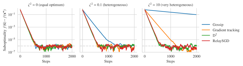
Figure 7: Random quadratics on ring networks of size 32 with varying data heterogeneity $\zeta^{2}$ and all other theoretical quantities fixed. To simulate stochastic noise, we add random normal noise to each gradient update. For each method, the learning rate is tuned to reach suboptimality $\leq 10^{-6}$ the fastest. RelaySGD operates on a chain network instead of a ring. Like D², it does not require more steps when the worker’s objectives are more heterogeneous.

E.4 Star topology

On star-topologies, the set of neighbors of worker 0 is $\{1,2,\ldots,n\}$ and the set of neighbors for every other worker is just $\{0\}$. While D² and RelaySGD are equally fast in the synthetic experiments on ring topologies in subsection E.3, RelaySGD is significantly faster on star topologies as illustrates by Figure 8.

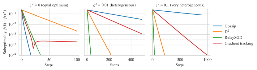
Figure 8: Random quadratics on star networks of size 32 with varying data heterogeneity $\zeta^{2}$ and all other theoretical quantities fixed. For each method, the learning rate is tuned to reach suboptimality $\leq 10^{-6}$ the fastest. Like D², RelaySGD does not require more steps when the worker’s objectives are more heterogeneous. Note that for $\zeta^{2}=0$ (left figure), our tuning procedure found a learning rate where Gradient Tracking does converge to $<\leq 10^{-6}$, but does not converge linearly. It would with a lower learning rate.

Appendix F RelaySum for distributed mean estimation

We conceptually separate the optimization algorithm RelaySGD from the communication mechanism RelaySum that uniformly distributes updates across a peer-to-peer network. We made this choice because we envision other applications of the RelaySum mechanism outside of optimization for machine learning. To illustrate this point, this section introduces RelaySum for Distributed Mean Estimation (Algorithm 5).

In distributed mean estimation, workers are connected in a network just as in our optimization setup, but instead of models gradients, they receive samples $\hat{\mathbf{d}}^{(t)}\sim\mathcal{D}$ of the distribution $\mathcal{D}$ at timestep $t$. The workers estimate the mean $\bar{\mathbf{d}}$ the mean of $\mathcal{D}$, and we measure their average squared error to the true mean.

Algorithm 5 RelaySum for Distributed Mean Estimation

1:$\forall~{}i,~{}\mathbf{x}_{i}^{(0)}=\mathbf{0},\mathbf{y}_{i}^{(0)}=\mathbf{0},s_{i}^{(0)}=0$; $\forall~{}i,j,\mathbf{m}^{(-1)}_{i\to j}=\mathbf{0}$, tree network

2:for $t=0,1,\ldots$ do

3:     for node $i$ in parallel

4:         for each neighbor $j\in\mathcal{N}_{i}$ do

5:              Get a sample $\hat{\mathbf{d}}_{i}^{(t)}\sim\mathcal{D}$.

6:              Send $\mathbf{m}^{(t)}_{i\to j}=\hat{\mathbf{d}}_{i}^{(t)}+\sum_{k\in\mathcal{N}_{i}\backslash j}\mathbf{m}^{(t-1)}_{k\to i}$.

7:              Send $c^{(t)}_{i\to j}=1+\sum_{k\in\mathcal{N}_{i}\backslash j}c^{(t-1)}_{k\to i}$.

8:              Receive $\mathbf{m}^{(t)}_{j\to i}$ and $c^{(t)}_{j\to i}$ from node $j$.

9:         end for

10:         Update the sum of samples $\mathbf{y}_{i}^{(t+1)}=\mathbf{y}_{i}^{(t)}+\hat{\mathbf{d}}_{i}^{(t)}+\sum_{j\in\mathcal{N}_{i}}\mathbf{m}_{j\to i}^{(t)}$.

11:         Update the sum of counts $s_{i}^{(t+1)}=s_{i}^{(t)}+1+\sum_{j\in\mathcal{N}_{i}}c_{j\to i}^{(t)}$.

12:         Output average estimate $\mathbf{x}_{i}^{(t)}=\mathbf{y}_{i}^{(t)}/s_{i}^{(t)}$

13:     end for

14:end for

In algorithm 5, the output estimates $\mathbf{x}_{i}^{(t)}$ of a worker $i$ is a uniform average of all samples that can reach a worker $i$ at that timestep. This algorithm enjoys variance reduction of $\mathcal{O}\left(\frac{1}{nT}\right)$, a desirable property that is in general not shared by gossip-averaging-based algorithms on arbitrary graphs.

In Figure 9, we compare this algorithm to a simple gossip-based baseline.

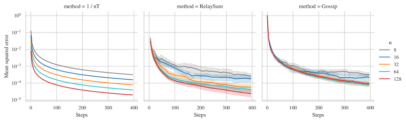
Figure 9: RelaySum for Distributed Mean Estimation compured to a gossip-based baseline, on a ring topology (chain for RelaySGD). Workers receive samples from a normal distribution $\mathcal{N}(1,1)$ with mean 1. RelaySum, using Algorithm 5 achieves a variance reduction of $\mathcal{O}\left(\frac{1}{nT}\right)$.

Appendix G Alternative optimizer based on RelaySum

Apart from RelaySGD presented in the main paper, there are other ways to build optimization algorithms based on the RelaySum communication mechanism. In this section, we describe RelaySGD/Grad (Algorithm 6), an alternative to RelaySGD that does uses the RelaySum mechanism on gradient updates rather than on models.

RelaySGD/Grad distributes each update uniformly over all workers in a finite number of steps. This means that worker’s models differ by only a finite number of $\mathcal{O}({\tau_{\max}}maxn)$ that are scaled as $\frac{1}{n}$. With this property, it achieves tighter consensus than typical gossip averaging, and it also works well in deep learning. Contrary to RelaySGD, however, this algorithm is not fully independent of data heterogeneity, due to the delay in the updates. When the data heterogeneity $\zeta^{2}>0$, RelaySGD/Grad does not converge linearly, but its suboptimality saturates at a level that depends on $\zeta^{2}$.

The sections below study this alternative algorithm in detail, both theoretically and experimentally. The key differences between RelaySGD and RelaySGD/Grad are:

	RelaySGD	RelaySGD/Grad
Provably independent of data heterogeneity $\zeta^{2}$	yes	no
Distributes updates exactly uniform in finite steps	no	yes
Loses energy of gradient updates (subsection D.1)	yes	no
Works experimentally with momentum / Adam	yes	no
Robust to lost messages + can support workers joining/leaving	yes	no

Algorithm 6 RelaySGD/Grad

1:$\forall~{}i,~{}\mathbf{x}_{i}^{(0)}=\mathbf{x}^{(0)}$; $\forall~{}i,j,\mathbf{m}^{(-1)}_{i\to j}=\mathbf{0}$, learning rate $\gamma$, tree network

2:for $t=0,1,\ldots$ do

3:     for node $i$ in parallel

4:         $\mathbf{u}_{i}^{(t)}=-\gamma\nabla f_{i}(\mathbf{x}_{i}^{(t)},\xi_{i}^{(t)})$

5:         for each neighbor $j\in\mathcal{N}_{i}$ do

6:              Send $\mathbf{m}^{(t)}_{i\to j}=\mathbf{u}_{i}^{(t)}+\sum_{k\in\mathcal{N}_{i}\backslash j}\mathbf{m}^{(t-1)}_{k\to i}$.

7:              Receive $\mathbf{m}^{(t)}_{j\to i}$ from node $j$.

8:         end for

9:         $\mathbf{x}_{i}^{(t+1)}=\mathbf{x}_{i}^{(t)}+\frac{1}{n}\left(\mathbf{u}_{i}^{(t)}+\sum_{j\in\mathcal{N}_{i}}\mathbf{m}_{j\to i}^{(t)}\right)$

10:     end for

11:end for

G.1 Theoretical analysis of RelaySGD/Grad

In this section we provide the theoretical analysis for RelaySGD/Grad. As the proof and analysis is very similar to [16], we only provide the case for the convex objective.

G.1.1 Proof of RelaySGD/Grad for the convex case

Let $\mathbf{x}^{\star}$ be the minimizer of $f$ and define the following iterates

• $r_{t}:=\operatorname{\mathbb{E}}\|\bar{\mathbf{x}}^{(t)}-\mathbf{x}^{\star}\|^{2}$,

• $e_{t}:=f(\bar{\mathbf{x}}^{(t)})-f(\mathbf{x}^{\star})$,

• $\Xi_{t}:=\frac{1}{n}\sum_{i=1}^{n}\|\mathbf{x}_{i}^{(t)}-\bar{\mathbf{x}}^{(t)}\|^{2}$.

Proposition X.

Let function $F_{i}(\mathbf{x},\xi)$, $i\in[n]$ be $L$-smooth (A) with bounded noise at the optimum (H). Then for any $\mathbf{x}_{i}\in\mathbb{R}^{d}$,

$$\operatorname{\mathbb{E}}_{\xi_{1}^{t},\ldots,\xi_{n}^{t}}\left\|\frac{1}{n}\sum_{i=1}^{n}(\nabla f_{i}(\mathbf{x}_{i}^{(t)})-\nabla F_{i}(\mathbf{x}_{i}^{(t)},\xi_{i}^{(t)}))\right\|^{2}\leq\tfrac{3}{n}(L^{2}\Xi_{t}+2Le_{t}+\bar{\sigma}^{2})$$

Proof.

In this proof we ignore the superscript $t$ as it does not raise embiguity.

$$\operatorname{\mathbb{E}}_{\xi_{1},\ldots,\xi_{n}}\left\|\frac{1}{n}\sum_{i=1}^{n}(\nabla f_{i}(\mathbf{x}_{i})-\nabla F_{i}(\mathbf{x}_{i},\xi_{i}))\right\|^{2}\leq\frac{1}{n^{2}}\sum_{i=1}^{n}\operatorname{\mathbb{E}}_{\xi_{i}}\|\nabla f_{i}(\mathbf{x}_{i})-\nabla F_{i}(\mathbf{x}_{i},\xi_{i})\|^{2}$$

$$= \frac{1}{n^{2}}\sum_{i=1}^{n}\operatorname{\mathbb{E}}_{\xi_{i}}\left\|\nabla f_{i}(\mathbf{x}_{i})-\nabla F_{i}(\mathbf{x}_{i},\xi_{i})\pm\nabla F_{i}(\bar{\mathbf{x}},\xi_{i})\pm\nabla f_{i}(\bar{\mathbf{x}})\pm\nabla F_{i}(\mathbf{x}^{\star},\xi_{i})\pm\nabla f_{i}(\mathbf{x}^{\star})\right\|^{2}$$

$$\leq \frac{3}{n^{2}}\sum_{i=1}^{n}\operatorname{\mathbb{E}}_{\xi_{i}}\left(\|\nabla f_{i}(\mathbf{x}_{i})-\nabla f_{i}(\bar{\mathbf{x}})+\nabla F_{i}(\bar{\mathbf{x}},\xi_{i})-\nabla F_{i}(\mathbf{x}_{i},\xi_{i})\|^{2}\right.$$

$$\qquad+\|\nabla f_{i}(\bar{\mathbf{x}})-\nabla f_{i}(\mathbf{x}^{\star})+\nabla F_{i}(\mathbf{x}^{\star},\xi_{i})-\nabla F_{i}(\bar{\mathbf{x}},\xi_{i})\|^{2}+\|\nabla f_{i}(\mathbf{x}^{\star})-\nabla F_{i}(\mathbf{x}^{\star},\mathbf{x}_{i})\|^{2})$$

$$\leq \frac{3}{n^{2}}\sum_{i=1}^{n}\operatorname{\mathbb{E}}_{\xi_{i}}(\|\nabla F_{i}(\mathbf{x}_{i},\xi_{i})-\nabla F_{i}(\bar{\mathbf{x}},\xi_{i})\|^{2}+\|\nabla F_{i}(\bar{\mathbf{x}},\xi_{i})-\nabla F_{i}(\mathbf{x}^{\star},\xi_{i})\|^{2}+\|\nabla F_{i}(\mathbf{x}^{\star},\mathbf{x}_{i})-\nabla f_{i}(\mathbf{x}^{\star})\|^{2})$$

$$\leq \frac{3}{n^{2}}\sum_{i=1}^{n}(L^{2}\|\mathbf{x}_{i}-\bar{\mathbf{x}}\|^{2}+2L(f_{i}(\bar{\mathbf{x}})-f_{i}(\mathbf{x}^{\star}))+\sigma_{i}^{2})$$

∎

Lemma 20.

(Descent lemma for convex objective.) If $\gamma\leq\frac{1}{10L}$, then

$$r_{t+1}\leq(1-\tfrac{\gamma\mu}{2})r_{t}-\gamma e_{t}+3\gamma L\Xi_{t}+\tfrac{3}{n}\gamma^{2}\bar{\sigma}^{2}.$$

Proof.

Throughout this proof we use $\operatorname{\mathbb{E}}=\operatorname{\mathbb{E}}_{\xi_{1}^{t},\ldots,\xi_{n}^{t}}$. Expand iterate $r_{t+1}=\operatorname{\mathbb{E}}\|\bar{\mathbf{x}}^{(t+1)}-\mathbf{x}^{\star}\|^{2}$

$$\operatorname{\mathbb{E}}\|\bar{\mathbf{x}}^{(t+1)}-\mathbf{x}^{\star}\|^{2}$$

$$= \operatorname{\mathbb{E}}\|\bar{\mathbf{x}}^{(t)}-\tfrac{\gamma}{n}\textstyle\sum\nolimits_{i=1}^{n}\nabla F_{i}(\mathbf{x}_{i}^{(t)},\xi_{i}^{(t)})\pm\tfrac{\gamma}{n}\textstyle\sum\nolimits_{i=1}^{n}\nabla f_{i}(\mathbf{x}_{i}^{(t)})-\mathbf{x}^{\star}\|^{2}$$

$$= \|\bar{\mathbf{x}}^{(t)}-\mathbf{x}^{\star}-\tfrac{\gamma}{n}\textstyle\sum\nolimits_{i=1}^{n}\nabla f_{i}(\mathbf{x}_{i}^{(t)})\|^{2}+\operatorname{\mathbb{E}}\|\tfrac{\gamma}{n}\textstyle\sum\nolimits_{i=1}^{n}\nabla F_{i}(\mathbf{x}_{i}^{(t)},\xi_{i}^{(t)})-\tfrac{\gamma}{n}\textstyle\sum\nolimits_{i=1}^{n}\nabla f_{i}(\mathbf{x}_{i}^{(t)})\|^{2}$$

$$+2\operatorname{\mathbb{E}}\langle\bar{\mathbf{x}}^{(t)}-\mathbf{x}^{\star}-\tfrac{\gamma}{n}\textstyle\sum\nolimits_{i=1}^{n}\nabla f_{i}(\mathbf{x}_{i}^{(t)}),\tfrac{\gamma}{n}\textstyle\sum\nolimits_{i=1}^{n}\nabla F_{i}(\mathbf{x}_{i}^{(t)},\xi_{i}^{(t)})-\tfrac{\gamma}{n}\textstyle\sum\nolimits_{i=1}^{n}\nabla f_{i}(\mathbf{x}_{i}^{(t)})\rangle$$

$$= \|\bar{\mathbf{x}}^{(t)}-\mathbf{x}^{\star}-\tfrac{\gamma}{n}\textstyle\sum\nolimits_{i=1}^{n}\nabla f_{i}(\mathbf{x}_{i}^{(t)})\|^{2}+\operatorname{\mathbb{E}}\|\tfrac{\gamma}{n}\textstyle\sum\nolimits_{i=1}^{n}\nabla F_{i}(\mathbf{x}_{i}^{(t)},\xi_{i}^{(t)})-\tfrac{\gamma}{n}\textstyle\sum\nolimits_{i=1}^{n}\nabla f_{i}(\mathbf{x}_{i}^{(t)})\|^{2}$$

The second term is bounded by Proposition X. Consider the first term

$$\|\bar{\mathbf{x}}^{(t)}-\mathbf{x}^{\star}-\tfrac{\gamma}{n}\textstyle\sum\nolimits_{i=1}^{n}\nabla f_{i}(\mathbf{x}_{i}^{(t)})\|^{2}$$

$$\leq \|\bar{\mathbf{x}}^{(t)}-\mathbf{x}^{\star}\|^{2}+\gamma^{2}\underbrace{\|\tfrac{1}{n}\textstyle\sum\nolimits_{i=1}^{n}\nabla f_{i}(\mathbf{x}_{i}^{(t)})\|^{2}}_{=:T_{1}}-2\gamma\underbrace{\langle\bar{\mathbf{x}}_{t}-\mathbf{x}^{\star},\tfrac{1}{n}\textstyle\sum\nolimits_{i=1}^{n}\nabla f_{i}(\mathbf{x}_{i}^{(t)})\rangle}_{=:T_{2}}.$$

First consider $T_{1}$,

$$T_{1} =\|\tfrac{1}{n}\textstyle\sum\nolimits_{i=1}^{n}(\nabla f_{i}(\mathbf{x}_{i}^{(t)})-\nabla f_{i}(\bar{\mathbf{x}}^{(t)})+\nabla f_{i}(\bar{\mathbf{x}}^{(t)})-\nabla f_{i}(\mathbf{x}^{\star}))\|^{2}$$

$$\leq\tfrac{2L^{2}}{n}\textstyle\sum\nolimits_{i=1}^{n}\|\mathbf{x}_{i}^{(t)}-\bar{\mathbf{x}}^{(t)}\|^{2}+\tfrac{2}{n}\sum_{i=1}^{n}\|\nabla f_{i}(\bar{\mathbf{x}}^{(t)})-\nabla f_{i}(\mathbf{x}^{\star})\|^{2}$$

$$\stackrel{{\scriptstyle\eqref{eq:smooth:optimum}}}{{\leq}}\tfrac{2L^{2}}{n}\textstyle\sum\nolimits_{i=1}^{n}\|\mathbf{x}_{i}^{(t)}-\bar{\mathbf{x}}^{(t)}\|^{2}+\tfrac{4L}{n}\sum_{i=1}^{n}(f_{i}(\bar{\mathbf{x}}^{(t)})-f_{i}(\mathbf{x}^{\star})-\langle\bar{\mathbf{x}}^{(t)}-\mathbf{x}^{\star},\nabla f_{i}(\mathbf{x}^{\star})\rangle)$$

$$=\tfrac{2L^{2}}{n}\textstyle\sum\nolimits_{i=1}^{n}\|\mathbf{x}_{i}^{(t)}-\bar{\mathbf{x}}^{(t)}\|^{2}+4L(f(\bar{\mathbf{x}}^{(t)})-f(\mathbf{x}^{\star}))$$

$$=2L^{2}\Xi_{t}+4Le_{t}.$$

Consider $T_{2}$,

$$T_{2} =\tfrac{1}{n}\textstyle\sum\nolimits_{i=1}^{n}(\langle\bar{\mathbf{x}}^{(t)}-\mathbf{x}_{i}^{(t)},\nabla f_{i}(\mathbf{x}_{i}^{(t)})\rangle+\langle\mathbf{x}_{i}^{(t)}-\mathbf{x}^{\star},\nabla f_{i}(\mathbf{x}_{i}^{(t)})\rangle)$$

$$\geq\tfrac{1}{n}\textstyle\sum\nolimits_{i=1}^{n}\left(f_{i}(\bar{\mathbf{x}}^{(t)})-f_{i}(\mathbf{x}_{i}^{(t)})-\tfrac{L}{2}\|\bar{\mathbf{x}}^{(t)}-\mathbf{x}_{i}^{(t)}\|^{2}+\langle\mathbf{x}_{i}^{(t)}-\mathbf{x}^{\star},\nabla f_{i}(\mathbf{x}_{i}^{(t)})\rangle\right)$$

$$\geq\tfrac{1}{n}\textstyle\sum\nolimits_{i=1}^{n}\left(f_{i}(\bar{\mathbf{x}}^{(t)})-f_{i}(\mathbf{x}_{i}^{(t)})-\tfrac{L}{2}\|\bar{\mathbf{x}}^{(t)}-\mathbf{x}_{i}^{(t)}\|^{2}+f_{i}(\mathbf{x}_{i}^{(t)})-f_{i}(\mathbf{x}^{\star})+\tfrac{\mu}{2}\|\mathbf{x}_{i}^{(t)}-\mathbf{x}^{\star}\|^{2}\right)$$

$$=f(\bar{\mathbf{x}}^{(t)})-f(\mathbf{x}^{\star})+\tfrac{1}{n}\textstyle\sum\nolimits_{i=1}^{n}\left(\tfrac{\mu}{2}\|\mathbf{x}_{i}^{(t)}-\mathbf{x}^{\star}\|^{2}-\tfrac{L}{2}\|\bar{\mathbf{x}}^{(t)}-\mathbf{x}_{i}^{(t)}\|^{2}\right)$$

$$\geq f(\bar{\mathbf{x}}^{(t)})-f(\mathbf{x}^{\star})+\tfrac{1}{n}\textstyle\sum\nolimits_{i=1}^{n}\left(\tfrac{\mu}{4}\|\bar{\mathbf{x}}^{(t)}-\mathbf{x}^{\star}\|^{2}-\tfrac{\mu+L}{2}\|\bar{\mathbf{x}}^{(t)}-\mathbf{x}_{i}^{(t)}\|^{2}\right)$$

$$\geq e_{t}+\tfrac{\mu}{4}r_{t}-L\Xi_{t}$$

where the first inequality and the second inequality uses the $L$-smoothness and $\mu$-convexity of $f_{i}$.

Combine both $T_{1}$, $T_{2}$ and Proposition X we have

$$r_{t+1} \leq r_{t}+\gamma^{2}(2L^{2}\Xi_{t}+4Le_{t})-2\gamma(e_{t}+\tfrac{\mu}{4}r_{t}-L\Xi_{t})+\tfrac{3}{n}\gamma^{2}(L^{2}\Xi_{t}+2Le_{t}+\bar{\sigma}^{2})$$

$$=(1-\tfrac{\gamma\mu}{2})r_{t}-2\gamma(1-5L\gamma)e_{t}+\gamma L(5\gamma L+2)\Xi_{t}+\tfrac{3}{n}\gamma^{2}\bar{\sigma}^{2}.$$

In addition if $\gamma\leq\frac{1}{10L}$, then

$$r_{t+1} \leq(1-\tfrac{\gamma\mu}{2})r_{t}-\gamma e_{t}+3\gamma L\Xi_{t}+\tfrac{3}{n}\gamma^{2}\bar{\sigma}^{2}.$$

∎

Lemma 21.

Bound the consensus distance as follows

$$\Xi_{t}\leq 3\gamma^{2}{\tau_{\max}}\textstyle\sum\nolimits_{t^{\prime}=[t-{\tau_{\max}}]^{+}}^{t-1}\left(2L^{2}\Xi_{t^{\prime}}+4L\mathbf{e}_{t^{\prime}}+(\bar{\sigma}^{2}+\bar{\zeta}^{2})\right).$$

Furthermore, multiply with a non-negative sequence $\{w_{t}\}_{t\geq 0}$ and average over time gives

$$\tfrac{1}{W_{T}}\textstyle\sum\nolimits_{t=0}^{T}w_{t}\Xi_{t} \leq\tfrac{1}{6LW_{T}}\textstyle\sum\nolimits_{t=0}^{T}w_{t}e_{t}+6\gamma^{2}{\tau_{\max}}^{2}(\bar{\sigma}^{2}+\bar{\zeta}^{2})$$

where $W_{T}:=\sum_{t=0}^{T}w_{t}$ and $\gamma\leq\frac{1}{10L{\tau_{\max}}}$.

Proof.

Throughout this proof we use $\operatorname{\mathbb{E}}=\operatorname{\mathbb{E}}_{\xi_{1}^{t},\ldots,\xi_{n}^{t}}$. Denote $[x]^{+}:=\max\{x,0\}$. For all $i\in[n]$,

$$\operatorname{\mathbb{E}}\lVert\mathbf{e}_{i}^{t}\rVert^{2}= \operatorname{\mathbb{E}}\lVert\tfrac{\gamma}{n}\textstyle\sum\nolimits_{j=1}^{n}\textstyle\sum\nolimits_{t^{\prime}=[t-{\tau_{\max}}_{ij}]^{+}}^{t-1}\nabla F_{j}(\mathbf{x}_{j}^{(t^{\prime})},\xi_{j}^{(t^{\prime})})\pm\nabla f_{j}(\mathbf{x}_{j}^{(t^{\prime})})\rVert^{2}$$

$$\leq \tfrac{\gamma^{2}}{n}\textstyle\sum\nolimits_{j=1}^{n}\operatorname{\mathbb{E}}\lVert\textstyle\sum\nolimits_{t^{\prime}=[t-{\tau_{\max}}_{ij}]^{+}}^{t-1}\nabla F_{j}(\mathbf{x}_{j}^{(t^{\prime})},\xi_{j}^{(t^{\prime})})\pm\nabla f_{j}(\mathbf{x}_{j}^{(t^{\prime})})\rVert^{2}$$

$$\leq \tfrac{\gamma^{2}{\tau_{\max}}}{n}\textstyle\sum\nolimits_{j=1}^{n}\textstyle\sum\nolimits_{t^{\prime}=[t-{\tau_{\max}}]^{+}}^{t-1}\operatorname{\mathbb{E}}\lVert\nabla F_{j}(\mathbf{x}_{j}^{(t^{\prime})},\xi_{j}^{(t^{\prime})})\pm\nabla f_{j}(\mathbf{x}_{j}^{(t^{\prime})})\rVert^{2}$$

$$= \tfrac{\gamma^{2}{\tau_{\max}}}{n}\textstyle\sum\nolimits_{j=1}^{n}\textstyle\sum\nolimits_{t^{\prime}=[t-{\tau_{\max}}]^{+}}^{t-1}\operatorname{\mathbb{E}}\lVert\nabla F_{j}(\mathbf{x}_{j}^{(t^{\prime})},\xi_{j}^{(t^{\prime})})-\nabla f_{j}(\mathbf{x}_{j}^{(t^{\prime})})\rVert^{2}$$

$$+\underbrace{\tfrac{\gamma^{2}{\tau_{\max}}}{n}\textstyle\sum\nolimits_{j=1}^{n}\textstyle\sum\nolimits_{t^{\prime}=[t-{\tau_{\max}}]^{+}}^{t-1}\lVert\nabla f_{j}(\mathbf{x}_{j}^{(t^{\prime})})\rVert^{2}}_{=:T_{3}}$$

We can apply Proposition X to the first term

$$\tfrac{\gamma^{2}{\tau_{\max}}}{n}\textstyle\sum\nolimits_{j=1}^{n}\textstyle\sum\nolimits_{t^{\prime}=[t-{\tau_{\max}}]^{+}}^{t-1}\operatorname{\mathbb{E}}\lVert\nabla F_{j}(\mathbf{x}_{j}^{(t^{\prime})},\xi_{j}^{(t^{\prime})})-\nabla f_{j}(\mathbf{x}_{j}^{(t^{\prime})})\rVert^{2}\leq 3\gamma^{2}{\tau_{\max}}\textstyle\sum\nolimits_{t^{\prime}=[t-{\tau_{\max}}]^{+}}^{t-1}(L^{2}\Xi_{t^{\prime}}+2L\mathbf{e}_{t^{\prime}}+\bar{\sigma}^{2}).$$

The second term $T_{3}$ can be bounded by adding $0=\pm\nabla f_{j}(\bar{\mathbf{x}}^{(t^{\prime})})\pm\nabla f_{j}(\mathbf{x}^{\star})$ inside the norm

$$T_{3} \leq\tfrac{\gamma^{2}{\tau_{\max}}}{n}\textstyle\sum\nolimits_{j=1}^{n}\textstyle\sum\nolimits_{t^{\prime}=[t-{\tau_{\max}}]^{+}}^{t-1}\lVert\nabla f_{j}(\mathbf{x}_{j}^{(t^{\prime})})\pm\nabla f_{j}(\bar{\mathbf{x}}^{(t^{\prime})})\pm\nabla f_{j}(\mathbf{x}^{\star})\rVert^{2}$$

$$\leq\tfrac{3\gamma^{2}{\tau_{\max}}}{n}\textstyle\sum\nolimits_{j=1}^{n}\sum_{t^{\prime}=[t-{\tau_{\max}}]^{+}}^{t-1}\left(L^{2}\lVert\mathbf{x}_{j}^{(t^{\prime})}-\bar{\mathbf{x}}^{(t^{\prime})}\rVert^{2}+\lVert\nabla f_{j}(\bar{\mathbf{x}}^{(t^{\prime})})-\nabla f_{j}(\mathbf{x}^{\star})\rVert^{2}+\lVert\nabla f_{j}(\mathbf{x}^{\star})\rVert^{2}\right)$$

$$=3\gamma^{2}{\tau_{\max}}\textstyle\sum\nolimits_{t^{\prime}=[t-{\tau_{\max}}]^{+}}^{t-1}\left(L^{2}\Xi_{t^{\prime}}+\tfrac{1}{n}\textstyle\sum\nolimits_{j=1}^{n}\lVert\nabla f_{j}(\bar{\mathbf{x}}^{(t^{\prime})})-\nabla f_{j}(\mathbf{x}^{\star})\rVert^{2}+\bar{\zeta}^{2}\right)$$

$$\stackrel{{\scriptstyle\eqref{eq:smooth:optimum}}}{{\leq}}3\gamma^{2}{\tau_{\max}}\textstyle\sum\nolimits_{t^{\prime}=[t-{\tau_{\max}}]^{+}}^{t-1}\left(L^{2}\Xi_{t^{\prime}}+2L(f(\bar{\mathbf{x}}^{(t^{\prime})})-f(\mathbf{x}^{\star}))+\bar{\zeta}^{2}\right)$$

Therefore

$$\operatorname{\mathbb{E}}\lVert\mathbf{e}_{i}^{t}\rVert^{2}\leq 3\gamma^{2}{\tau_{\max}}\textstyle\sum\nolimits_{t^{\prime}=[t-{\tau_{\max}}]^{+}}^{t-1}(2L^{2}\Xi_{t^{\prime}}+4L\mathbf{e}_{t^{\prime}}+(\bar{\sigma}^{2}+\bar{\zeta}^{2})).$$

Average over $i$ on both sides and note the right hand side does not depend on index $i$,

$$\Xi_{t}=\tfrac{1}{n}\textstyle\sum\nolimits_{i=1}^{n}\|\mathbf{e}_{i}^{t}\|^{2}\leq 3\gamma^{2}{\tau_{\max}}\sum_{t^{\prime}=[t-{\tau_{\max}}]^{+}}^{t-1}\left(2L^{2}\Xi_{t^{\prime}}+4L\mathbf{e}_{t^{\prime}}+\bar{\sigma}^{2}\right).$$

Multiply both sides by $w_{t}$ and sum over $t$ gives

$$\tfrac{1}{W_{T}}\textstyle\sum\nolimits_{t=0}^{T}w_{t}\Xi_{t} \leq\tfrac{3\gamma^{2}{\tau_{\max}}^{2}}{W_{T}}\textstyle\sum\nolimits_{t=0}^{T}w_{t}\left(2L^{2}\Xi_{t}+4Le_{t}+\bar{\sigma}^{2}\right)$$

$$=\tfrac{6\gamma^{2}L^{2}{\tau_{\max}}^{2}}{W_{T}}\textstyle\sum\nolimits_{t=0}^{T}w_{t}\Xi_{t}+\tfrac{12\gamma^{2}L{\tau_{\max}}^{2}}{W_{T}}\sum_{t=0}^{T}w_{t}e_{t}+3\gamma^{2}{\tau_{\max}}(\bar{\sigma}^{2}+\bar{\zeta}^{2})$$

where $W_{T}:=\sum_{t=0}^{T}w_{t}$. Rearrage the terms and let $\gamma\leq\frac{1}{10L{\tau_{\max}}}$ give

$$\tfrac{1}{W_{T}}\textstyle\sum\nolimits_{t=0}^{T}w_{t}\Xi_{t} \leq\frac{1}{1-6\gamma^{2}L^{2}{\tau_{\max}}^{2}}\left(\tfrac{12\gamma^{2}L{\tau_{\max}}^{2}}{W_{T}}\textstyle\sum\nolimits_{t=0}^{T}w_{t}e_{t}+\tfrac{3\gamma^{2}{\tau_{\max}}^{2}}{n}(\bar{\sigma}^{2}+\bar{\zeta}^{2})\right)$$

$$\leq\tfrac{1}{6LW_{T}}\textstyle\sum\nolimits_{t=0}^{T}w_{t}e_{t}+6\gamma^{2}{\tau_{\max}}^{2}(\bar{\sigma}^{2}+\bar{\zeta}^{2})$$

∎

Theorem XI.

For convex objective, we have

$$\frac{1}{T+1}\sum_{t=0}^{T}\left(f(\bar{\mathbf{x}}^{(t)})-f(\mathbf{x}^{\star})\right)\leq 4\left(\frac{3\bar{\sigma}^{2}r_{0}}{n(T+1)}\right)^{\frac{1}{2}}+4\left(\frac{6{\tau_{\max}}\sqrt{L(\bar{\sigma}^{2}+\bar{\zeta}^{2})}r_{0}}{T+1}\right)^{\frac{2}{3}}+\frac{10L(\tau_{\max}+1)r_{0}}{T+1}.$$

where $r_{0}=\|\mathbf{x}^{0}-\mathbf{x}^{\star}\|^{2}$.

Remark 22.

For target accuracy $\varepsilon>0$, then $\frac{1}{T+1}\sum_{t=0}^{T}\left(f(\bar{\mathbf{x}}^{(t)})-f(\mathbf{x}^{\star})\right)<\varepsilon$ after

$$\mathcal{O}\left(\frac{\bar{\sigma}^{2}r_{0}}{n\varepsilon^{2}}+\frac{\tau_{\max}\sqrt{L(\bar{\sigma}^{2}+\bar{\zeta}^{2})}r_{0}}{\varepsilon^{3/2}}+\frac{10L(\tau_{\max}+1)r_{0}}{\varepsilon}\right)$$

iterations. This result is similar to [16, Theorem 2] except that here we replace spectral gap $p$ with the inverse of maximum delay $\frac{1}{\tau_{\max}}$.

Proof.

Consider Lemma 20 and multiply both sides with $\frac{w_{t}}{\gamma}$ and average over time

$$\tfrac{1}{W_{T}}\textstyle\sum\nolimits_{t=0}^{T}w_{t}e_{t} \leq\tfrac{1}{W_{T}}\textstyle\sum\nolimits_{t=0}^{T}(\tfrac{w_{t}}{\gamma}r_{t}-\tfrac{w_{t}}{\gamma}r_{t+1})+\tfrac{3L}{W_{T}}\textstyle\sum\nolimits_{t=0}^{T}w_{t}\Xi_{t}+\tfrac{3\gamma}{nW_{T}}\textstyle\sum\nolimits_{t=0}^{T}w_{t}\bar{\sigma}^{2}$$

$$\leq\tfrac{1}{W_{T}}\textstyle\sum\nolimits_{t=0}^{T}(\tfrac{w_{t}}{\gamma}r_{t}-\tfrac{w_{t}}{\gamma}r_{t+1})+\tfrac{1}{2W_{T}}\textstyle\sum\nolimits_{t=0}^{T}w_{t}e_{t}+18\gamma^{2}{\tau_{\max}}^{2}L(\bar{\sigma}^{2}+\bar{\zeta}^{2})+\tfrac{3\gamma\bar{\sigma}^{2}}{n}$$

where the second inequality comes from Lemma 21. Then

$$\tfrac{1}{2W_{T}}\textstyle\sum\nolimits_{t=0}^{T}w_{t}e_{t} \leq\tfrac{1}{W_{T}}\textstyle\sum\nolimits_{t=0}^{T}(\tfrac{w_{t}}{\gamma}r_{t}-\tfrac{w_{t}}{\gamma}r_{t+1}+\tfrac{3\bar{\sigma}^{2}}{n}\gamma+18{\tau_{\max}}^{2}L(\bar{\sigma}^{2}+\bar{\zeta}^{2})\gamma^{2}).$$

We can further consider

$$\tfrac{3L}{W_{T}}\textstyle\sum\nolimits_{t=0}^{T}w_{t}\Xi_{t}= \tfrac{1}{2W_{T}}\textstyle\sum\nolimits_{t=0}^{T}w_{t}e_{t}+18{\tau_{\max}}^{2}L(\bar{\sigma}^{2}+\bar{\zeta}^{2})\gamma^{2}$$

$$\leq \tfrac{1}{W_{T}}\textstyle\sum\nolimits_{t=0}^{T}(\tfrac{w_{t}}{\gamma}r_{t}-\tfrac{w_{t}}{\gamma}r_{t+1}+\tfrac{3\bar{\sigma}^{2}}{n}\gamma+36{\tau_{\max}}^{2}L(\bar{\sigma}^{2}+\bar{\zeta}^{2})\gamma^{2})=:\Psi_{T}.$$

Taking $\{w_{t}=1\}_{t\geq 0}$, then

$$\Psi_{T}\leq\tfrac{r_{0}}{\gamma(T+1)}+\tfrac{3\bar{\sigma}^{2}}{n}\gamma+36{\tau_{\max}}^{2}L(\bar{\sigma}^{2}+\bar{\zeta}^{2})\gamma^{2}.$$

Apply Lemma 16 we have

$$\Psi_{T}\leq 2\left(\frac{3\bar{\sigma}^{2}r_{0}}{n(T+1)}\right)^{\frac{1}{2}}+2\left(\frac{6{\tau_{\max}}\sqrt{L(\bar{\sigma}^{2}+\bar{\zeta}^{2})}r_{0}}{T+1}\right)^{\frac{2}{3}}+\frac{dr_{0}}{T+1}.$$

where $d=\max\{10L,10L{\tau_{\max}}\}\leq 10L(\tau_{\max}+1)$ and at the same time

$$\frac{1}{2(T+1)}\sum_{t=0}^{T}e_{t}\leq 2\left(\frac{3\bar{\sigma}^{2}r_{0}}{n(T+1)}\right)^{\frac{1}{2}}+2\left(\frac{6{\tau_{\max}}\sqrt{L(\bar{\sigma}^{2}+\bar{\zeta}^{2})}r_{0}}{T+1}\right)^{\frac{2}{3}}+\frac{dr_{0}}{T+1}$$

$$\frac{3L}{T+1}\sum_{t=0}^{T}\Xi_{t}\leq 2\left(\frac{3\bar{\sigma}^{2}r_{0}}{n(T+1)}\right)^{\frac{1}{2}}+2\left(\frac{6{\tau_{\max}}\sqrt{L(\bar{\sigma}^{2}+\bar{\zeta}^{2})}r_{0}}{T+1}\right)^{\frac{2}{3}}+\frac{dr_{0}}{T+1}$$

∎

G.2 Empirical analysis of RelaySGD/Grad

In Table 14, we compare RelaySGD/Grad to RelaySGD on deep-learning based image classification on Cifar-10 with VGG-11. Without momentum, and with low levels of heterogeneity, RelaySGD/Grad sometimes outperforms RelaySGD.

Figure 10 illustrates a key difference between RelaySGD/Grad and RelaySGD. While RelaySGD behaves independently of heterogeneity, and converges linearly with a fixed step size, RelaySGD/Grad reaches a plateau based on the learning rate and level of heterogeneity.

Table 14: Comparing RelaySGD/Grad with RelaySGD on Cifar-10 [17] with the VGG-11 architecture. We vary the data heterogeneity $\alpha$ [20] between 16 workers. For low-heterogeneity cases and without momentum, RelaySGD/Grad sometimes performs better than RelaySGD.

Algorithm	Topology	$\alpha=1.00$	$\alpha=0.1$	$\alpha=.01$
		(most homogeneous)		(most heterogeneous)
All-reduce (baseline)	fully connected	87.0%	87.0%	87.0%
$\quad+$momentum		90.2%	90.2%	90.2%
RelaySGD	chain	87.3%	87.2%	86.5%
$\quad+$local momentum		89.5%	89.2%	88.4%
RelaySGD/Grad	chain	88.8%	88.5%	83.5%
$\quad+$local momentum		86.9%	87.8%	68.6%

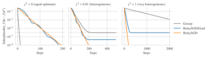
Figure 10: Comparing RelaySGD/Grad against RelaySGD on random quadratics with varying levels of heterogeneity $\zeta^{2}$, without stochastic noise, on a ring/chain of 32 nodes. Learning rates are tuned to reach suboptimality $\leq 10^{-6}$ as quickly as possible. In contrast to RelaySGD, RelaySGD/Grad with a fixed learning rate does not converge linearly. Compared to DP-SGD (Gossip), RelaySGD/Grad is still less sensitive to data heterogeneity.

References

- Agarwal and Duchi [2012] Alekh Agarwal and John C. Duchi. Distributed delayed stochastic optimization. In Proc. CDC, pages 5451–5452, 2012.
- Assran et al. [2019] Mahmoud Assran, Nicolas Loizou, Nicolas Ballas, and Michael G. Rabbat. Stochastic gradient push for distributed deep learning. In Proc. ICML, volume 97, pages 344–353, 2019.
- Ba et al. [2016] Jimmy Lei Ba, Jamie Ryan Kiros, and Geoffrey E Hinton. Layer normalization. In ICLR, 2016.
- Davis et al. [1930] Allison Davis, Burleigh Bradford Gardner, and Mary R Gardner. Deep South: A social anthropological study of caste and class. Univ of South Carolina Press, 1930.
- Deng et al. [2009] Jia Deng, Wei Dong, Richard Socher, Li-Jia Li, Kai Li, and Fei-Fei Li. Imagenet: A large-scale hierarchical image database. In Proc. CVPR, pages 248–255, 2009.
- Georgopoulos [2011] Leonidas Georgopoulos. Definitive Consensus for Distributed Data Inference. PhD thesis, EPFL, 2011.
- Hagberg et al. [2008] Aric Hagberg, Pieter Swart, and Daniel S Chult. Exploring network structure, dynamics, and function using NetworkX. Technical report, Los Alamos National Lab.(LANL), Los Alamos, NM (United States), 2008.
- Hendrickx et al. [2014] Julien M. Hendrickx, Raphaël M. Jungers, Alexander Olshevsky, and Guillaume Vankeerberghen. Graph diameter, eigenvalues, and minimum-time consensus. Automatica, 50(2):635–640, 2014.
- Ioffe and Szegedy [2015] Sergey Ioffe and Christian Szegedy. Batch normalization: Accelerating deep network training by reducing internal covariate shift. In Proc. ICML, volume 37, pages 448–456, 2015.
- Jeaugey [2019] Sylvain Jeaugey. Massively scale your deep learning training with NCCL 2.4. https://devblogs.nvidia.com/massively-scale-deep-learning-training-nccl-2-4/, 2019. [Online; accessed 21-May-2019].
- Johansson et al. [2009] Björn Johansson, Maben Rabi, and Mikael Johansson. A randomized incremental subgradient method for distributed optimization in networked systems. SIAM J. Optim., 20(3):1157–1170, 2009.
- Kairouz et al. [2019] Peter Kairouz, H. Brendan McMahan, Brendan Avent, Aurélien Bellet, Mehdi Bennis, Arjun Nitin Bhagoji, Keith Bonawitz, Zachary Charles, Graham Cormode, Rachel Cummings, Rafael G. L. D’Oliveira, Salim El Rouayheb, David Evans, Josh Gardner, Zachary Garrett, Adrià Gascón, Badih Ghazi, Phillip B. Gibbons, Marco Gruteser, Zaïd Harchaoui, Chaoyang He, Lie He, Zhouyuan Huo, Ben Hutchinson, Justin Hsu, Martin Jaggi, Tara Javidi, Gauri Joshi, Mikhail Khodak, Jakub Konecný, Aleksandra Korolova, Farinaz Koushanfar, Sanmi Koyejo, Tancrède Lepoint, Yang Liu, Prateek Mittal, Mehryar Mohri, Richard Nock, Ayfer Özgür, Rasmus Pagh, Mariana Raykova, Hang Qi, Daniel Ramage, Ramesh Raskar, Dawn Song, Weikang Song, Sebastian U. Stich, Ziteng Sun, Ananda Theertha Suresh, Florian Tramèr, Praneeth Vepakomma, Jianyu Wang, Li Xiong, Zheng Xu, Qiang Yang, Felix X. Yu, Han Yu, and Sen Zhao. Advances and open problems in federated learning. arXiv, abs/1912.04977, 2019.
- Kempe et al. [2003] David Kempe, Alin Dobra, and Johannes Gehrke. Gossip-based computation of aggregate information. In FOCS, pages 482–491, 2003.
- Kingma and Ba [2015] Diederik P. Kingma and Jimmy Ba. Adam: A method for stochastic optimization. In ICLR, 2015.
- Ko [2010] Chih-Kai Ko. On Matrix Factorization and Scheduling forFinite-time Average-consensus. PhD thesis, California Institute of Technology, 2010.
- Koloskova et al. [2020] Anastasia Koloskova, Nicolas Loizou, Sadra Boreiri, Martin Jaggi, and Sebastian U. Stich. A unified theory of decentralized SGD with changing topology and local updates. In Proc. ICML, volume 119, pages 5381–5393, 2020.
- Krizhevsky [2012] Alex Krizhevsky. Learning multiple layers of features from tiny images. University of Toronto, 05 2012.
- [18] Alex Krizhevsky, Vinod Nair, and Geoffrey Hinton. Cifar-10 (Canadian Institute for Advanced Research).
- Lian et al. [2017] Xiangru Lian, Ce Zhang, Huan Zhang, Cho-Jui Hsieh, Wei Zhang, and Ji Liu. Can decentralized algorithms outperform centralized algorithms? A case study for decentralized parallel stochastic gradient descent. In NeurIPS, pages 5330–5340, 2017.
- Lin et al. [2021] Tao Lin, Sai Praneeth Karimireddy, Sebastian U. Stich, and Martin Jaggi. Quasi-global momentum: Accelerating decentralized deep learning on heterogeneous data. CoRR, abs/2102.04761, 2021.
- Liu et al. [2020] Hanxiao Liu, Andy Brock, Karen Simonyan, and Quoc Le. Evolving normalization-activation layers. In NeurIPS, 2020.
- Lorenzo and Scutari [2016] Paolo Di Lorenzo and Gesualdo Scutari. Next: In-network nonconvex optimization. IEEE Transactions on Signal and Information Processing over Networks, 2(2):120–136, 2016.
- Lu and De Sa [2021] Yucheng Lu and Christopher De Sa. Optimal complexity in decentralized training. In Proc. ICML, volume 139, pages 7111–7123, 18–24 Jul 2021.
- McMahan et al. [2017] Brendan McMahan, Eider Moore, Daniel Ramage, Seth Hampson, and Blaise Agüera y Arcas. Communication-efficient learning of deep networks from decentralized data. In Proc. ICOAI, volume 54, pages 1273–1282, 2017.
- Nedic [2020] Angelia Nedic. Distributed gradient methods for convex machine learning problems in networks: Distributed optimization. IEEE Signal Process. Mag., 37(3):92–101, 2020.
- Nedic and Olshevsky [2016] Angelia Nedic and Alex Olshevsky. Stochastic gradient-push for strongly convex functions on time-varying directed graphs. IEEE Trans. Autom. Control., 61(12):3936–3947, 2016.
- Nedić and Ozdaglar [2010] Angelia Nedić and Asuman Ozdaglar. Convergence rate for consensus with delays. Journal of Global Optimization, 47(3):437–456, 2010.
- Nedic and Ozdaglar [2009] Angelia Nedic and Asuman E. Ozdaglar. Distributed subgradient methods for multi-agent optimization. IEEE Trans. Autom. Control., 54(1):48–61, 2009.
- Nedic et al. [2017] Angelia Nedic, Alex Olshevsky, and Wei Shi. Achieving geometric convergence for distributed optimization over time-varying graphs. SIAM J. Optim., 27(4):2597–2633, 2017.
- Perlman [1985] Radia J. Perlman. An algorithm for distributed computation of a spanningtree in an extended LAN. In SIGCOMM, pages 44–53, 1985.
- Pu and Nedic [2018] Shi Pu and Angelia Nedic. Distributed stochastic gradient tracking methods. CoRR, abs/1805.11454, 2018.
- Pu et al. [2021] Shi Pu, Wei Shi, Jinming Xu, and Angelia Nedic. Push-pull gradient methods for distributed optimization in networks. IEEE Trans. Autom. Control., 66(1):1–16, 2021.
- Sanders et al. [2009] Peter Sanders, Jochen Speck, and Jesper Larsson Träff. Two-tree algorithms for full bandwidth broadcast, reduction and scan. Parallel Comput., 35(12):581–594, 2009.
- Sanh et al. [2019] Victor Sanh, Lysandre Debut, Julien Chaumond, and Thomas Wolf. Distilbert, a distilled version of BERT: smaller, faster, cheaper and lighter. CoRR, abs/1910.01108, 2019.
- Stich [2019] Sebastian U. Stich. Unified optimal analysis of the (stochastic) gradient method. CoRR, abs/1907.04232, 2019.
- Tang et al. [2018] Hanlin Tang, Xiangru Lian, Ming Yan, Ce Zhang, and Ji Liu. D: Decentralized training over decentralized data. In Proc. ICML, volume 80, pages 4855–4863, 2018.
- Tsianos and Rabbat [2011] Konstantinos I. Tsianos and Michael G. Rabbat. Distributed consensus and optimization under communication delays. In Allerton, pages 974–982, 2011.
- Tsianos et al. [2012] Konstantinos I. Tsianos, Sean F. Lawlor, and Michael G. Rabbat. Push-sum distributed dual averaging for convex optimization. In Proc. CDC, pages 5453–5458, 2012.
- Xi and Khan [2017] Chenguang Xi and Usman A. Khan. DEXTRA: A fast algorithm for optimization over directed graphs. IEEE Trans. Automat. Contr., 62(10):4980–4993, 2017.
- Xi et al. [2018] Chenguang Xi, Van Sy Mai, Ran Xin, Eyad H. Abed, and Usman A. Khan. Linear convergence in optimization over directed graphs with row-stochastic matrices. IEEE Trans. Autom. Control., 63(10):3558–3565, 2018.
- Xiao and Boyd [2004] Lin Xiao and Stephen P. Boyd. Fast linear iterations for distributed averaging. Syst. Control. Lett., 53(1):65–78, 2004.
- Xin and Khan [2018] Ran Xin and Usman A. Khan. A linear algorithm for optimization over directed graphs with geometric convergence. IEEE Control. Syst. Lett., 2(3):315–320, 2018.
- Xin and Khan [2020] Ran Xin and Usman A. Khan. Distributed heavy-ball: A generalization and acceleration of first-order methods with gradient tracking. IEEE Trans. Autom. Control., 65(6):2627–2633, 2020.
- Xin et al. [2019] Ran Xin, Chenguang Xi, and Usman A. Khan. FROST - fast row-stochastic optimization with uncoordinated step-sizes. EURASIP J. Adv. Signal Process., 2019:1, 2019.
- Yuan et al. [2019] Kun Yuan, Bicheng Ying, Xiaochuan Zhao, and Ali H. Sayed. Exact diffusion for distributed optimization and learning - part I: algorithm development. IEEE Trans. Signal Process., 67(3):708–723, 2019.
- Yuan et al. [2021] Kun Yuan, Yiming Chen, Xinmeng Huang, Yingya Zhang, Pan Pan, Yinghui Xu, and Wotao Yin. Decentlam: Decentralized momentum SGD for large-batch deep training. CoRR, abs/2104.11981, 2021.
- Yurochkin et al. [2019] Mikhail Yurochkin, Mayank Agarwal, Soumya Ghosh, Kristjan H. Greenewald, Trong Nghia Hoang, and Yasaman Khazaeni. Bayesian nonparametric federated learning of neural networks. In Proc. ICML, volume 97, pages 7252–7261, 2019.
- Zhang and You [2020] Jiaqi Zhang and Keyou You. Decentralized stochastic gradient tracking for non-convex empirical risk minimization, 2020.
- Zhang et al. [2015] Xiang Zhang, Junbo Jake Zhao, and Yann LeCun. Character-level convolutional networks for text classification. In NeurIPS, pages 649–657, 2015.
- Zhang et al. [2019] Zhaorong Zhang, Kan Xie, Qianqian Cai, and Minyue Fu. A bp-like distributed algorithm for weighted average consensus. In Proc. ASCC, pages 728–733, 2019.