Multi-resolution Dynamic Mode Decomposition for
Damage Detection in Wind Turbine Gearboxes

Abstract

We introduce an approach for damage detection in gearboxes based on the analysis of sensor data with the multi-resolution dynamic mode decomposition (mrDMD). The application focus is the condition monitoring of wind turbine gearboxes under varying load conditions, in particular irregular and stochastic wind fluctuations. We analyze data stemming from a simulated vibration response of a simple nonlinear gearbox model in a healthy and damaged scenario and under different wind conditions. With mrDMD applied on time-delay snapshots of the sensor data, we can extract components in these vibration signals that highlight features related to damage and enable its identification. A comparison with Fourier analysis, Time Synchronous Averaging and Empirical Mode Decomposition shows the advantages of the proposed mrDMD-based data analysis approach for damage detection.

1 Introduction

The condition monitoring of wind turbine gearboxes presents a challenging scenario that is often not amenable to classical data analysis techniques due to the existing operating conditions. Note that wind turbines are one of the main sources of renewable energy (Redl et al.,, 2021) nowadays and gearbox-related defects are among those problems with the highest amount of downtime hours per failure (Dao et al.,, 2019). Therefore, damage detection in gearboxes is a significant aspect for keeping wind energy production high. To cope with the difficulties in the sensor signals, arising due to the prevailing wind fluctuations, we propose an approach for damage detection in gearboxes based on the analysis of sensor data with the multi-resolution dynamic mode decomposition (mrDMD).

Sensor data analysis is widely used to determine the health condition of mechanical devices. Analyzing the data generated by sensors installed on these devices, it is possible to continually monitor their integrity and detect anomalous behaviours, damages, and faults when they arise. Optimizing the monitoring process is of great interest because detecting damages in their early stage empowers companies to prevent more severe problems that could lead to a significant loss in terms of energy production and money.

Damage detection in gearbox vibration signals is a relatively easy task in steady operating conditions, as for example in a laboratory, see Doebling et al., (1996) for an overview of established methods. Unfortunately, when we deal with wind turbines, steady operating conditions represent an unrealistic scenario that does not take into account weather condition, temperature variation, and, most importantly, wind turbulence, all of which results in varying load conditions on the blades of the wind turbine. These factors strongly affect gearbox vibration signals, introducing a stochastic component that makes them non-deterministic and far from smooth. In this scenario damage detection is a much more difficult task since the data analysis strategies have not only to deal with signal anomalies induced by damage, but also by wind turbulence.

In this work, we consider the gearbox model and the scenario developed in Kahraman and Singh, (1991) and further refined in Antoniadou et al., (2015). The numerically produced signals include a stochastic component simulating the varying load condition caused by wind turbulence. Several kinds of damage can appear in gearboxes, here we focus on the crack of a gear’s tooth. The crack of a gear’s tooth is a bending fatigue failure. Bending fatigue failures usually occur in three progressive stages: crack initiation, crack propagation and tooth fracture or breakage (Errichello,, 2002). According to Ma et al., (2014) “Tooth fracture is the most serious fault in gearbox and it may cause complete failure of the gear”. Thus, the crack of a gear’s tooth is a damage in its early stage because the continuous interaction of the cracked tooth with the other gear leads to a progressive propagation of the crack until the breakage of the tooth occurs, leading to more severe damage that may even cause the total failure of the gear.

Historically speaking, fault detection in gearboxes was first performed using methods that focus on analyzing the spectral properties of sensor signals (Kumar et al.,, 2021), such as the Fast Fourier transform (Rao et al.,, 2011) and Cepstrum analysis (Badaoui et al.,, 2004). However, in the scenario we consider, these methods are strongly challenged by weather conditions, such as wind turbulence and temperature variation, which induce a stochastic component to the signals studied, changing their spectra non-deterministically over time. This stochastic change of the signals’ spectral properties strongly affects the effectiveness and reliability of spectral methods (Kumar et al.,, 2021). Empirical mode decomposition (EMD) (Huang et al.,, 1998) was proposed as an alternative to overcome the issues arising when studying spectral characteristics of signals. In the case of a damaged gearbox, EMD separates the time-domain signals in several modes that may contain damage features and may be used to detect faults. Unfortunately, EMD is affected by the so called “mode mixing problem”. The problem consists of the fact that the modes produced by EMD either contain information of the signal relative to widely disparate time-scales or similar time-scale information resides in different modes (Wu and Huang,, 2009; Xu et al.,, 2016). The main implications are that the physical meaning of each mode is unclear and that a proper interpretation of the information they contain is not a trivial task. This does not mean that such modes cannot be studied or selected according to some specific strategy in order to extract meaningful insights about the data, it rather means that there is no principled way to do that.

In this work we propose multi-resolution dynamic mode decomposition (mrDMD) (Kutz et al., 2016b, ), a variation of dynamic mode decomposition (DMD) (Schmid,, 2010), as an alternative to EMD that incorporates all its advantages and overcomes the mode mixing problem as well. mrDMD is a data-driven algorithm that has been used to perform different tasks, such as: spatio-temporal filtering of video or multi-scale separation of complex weather systems (Kutz et al., 2016b, ). We propose it as a novel approach to detect the crack of a tooth in a wind turbine gearbox by analyzing gearbox vibration signals generated under varying load conditions. mrDMD is able to decompose the signal in spatio-temporal modes that capture its geometrical characteristics in the time-domain at different time-scales. The difference to EMD is that it associates to each of its modes a complex number that could either represent a frequency or an energy content, according to the point of view one wants to consider, and thanks to this additional information high/low-frequency or energy content separation of the modes is possible. On the one hand, low-frequency modes represent those structures that vary slowly over time, which therefore are not affected by the non-deterministic variation caused by wind turbulence that mainly influences the signal at smaller time-scales. On the other hand, high-frequency modes represent those structures that evolve at higher frequencies and are strongly affected by wind turbulence and sudden changes in the gear stiffness caused by the cracked tooth we want to identify. We will see that computing the instantaneous amplitude of high-frequency modes, via the Hilbert Transform (HT), will enable us to easily identify anomalies arising in vibration signals from the crack of a gear’s tooth.

We aim to show the potential of mrDMD as a fault detection method, in a context in which the analyzed vibration signals are affected by stochastic perturbations. We study the proposed approach on simulated signals representing the vibration response of a simple gearbox model with two spur gears, as well on experimental data under controlled situations from a benchmark study.

The next sections are organized as follows: Section 2 presents an overview of related work on the topic of early damage detection in wind turbine gearboxes under varying load condition. Section 3 introduces our mrDMD based strategy for tooth damage identification. In Section 4 the gearbox model is introduced and numerical simulations of acceleration signals representing the vibration response of the modelled gearbox are considered. Finally, Section 5 demonstrates the performance of our method, and shows the issues the fast Fourier transform as a spectral method, an approach based on Time Synchronous Averaging, and an EMD-based approach experience by the presence of wind fluctuations.

2 Related work

Generally speaking, condition monitoring methods consist of damage detection methods, with the difference that one knows a priori about the frequency bands related to damage for the different monitored components. Reviews of methods used for damage detection in wind turbines can be found in Doebling et al., (1996); Kumar et al., (2021); Salameh et al., (2018); Sharma, (2021). The most classical techniques used for condition monitoring, and more in general for damage detection, mainly focus on analyzing the spectral characteristics of vibration signals, such as the spectral Kurtosis (Antoni,, 2006), Fourier analysis and modulation sidebands (Inalpolat and Kahraman,, 2010) and Cepstrum analysis (Badaoui et al.,, 2004). These methods have proven their capability to provide good results in identifying damages under simplified conditions, such as steady loading of the gearboxes. However, when considering time-varying load conditions, the spectral characteristics of gearbox vibration signals change non-deterministically with time. This stochastic behaviour can not be handled using Fourier analysis as the Fourier transform expands a signal as a linear combination of wave functions with constant frequency over time. To overcome this issue, many time-frequency methods have been employed in damage detection, such as: the Wigner–Ville distribution (Staszewski et al.,, 1997), the Vold–Kalman filter (Feng et al.,, 2019), wavelet analysis (Staszewski and Tomlinson,, 1994) and cyclostationary analysis (Antoni and Randall,, 2002; Xin et al.,, 2020). Probably, the most popular and successful of these methods is wavelet analysis (Hu et al.,, 2018; Peng and Chu,, 2004). Nonetheless, in the context we are considering, such a method has the disadvantage of relying on a fixed set of basis functions. This fact has a detrimental effect on its effectiveness and reliability in processing signals affected by perturbations of stochastic nature and that have spectral properties that change randomly with time. An additional approach to perform fault detection is given by entropy analysis (Sharma and Parey,, 2016). However, many entropy features are available for different types of faults, and it is not clear what are the right features for a given fault. Moreover, under varying load condition, the stochastic behaviour of the signal affects the performance of entropies which may show insignificant results, hence making them non-reliable (Sharma,, 2021; Sharma and Parey,, 2016). Another major contribution to the gear diagnostics filed is Time Synchronous Averaging (TSA) (Randall,, 2021). TSA is used to extract signal components associated with certain frequencies, as the meshing frequency, that may highlight damage features. Unfortunately, also this technique rely on being able to analyse signals recorded under steady speed and load conditions and it is strongly affected by the fluctuating operating conditions caused by wind turbulence.

Other strategies for damage detection, which try to overcome the problems experienced with TSA, entropy analysis and time-frequency methods, are based on the empirical mode decomposition (EMD) (Huang et al.,, 1998). The main advantage of using EMD with respect to entropy analysis and time-frequency methods is that it decomposes the signal into several components, or modes, which may contain meaningful information related to damage. After decomposing the vibration signal, the instantaneous frequency and amplitude of each component can be estimated, most commonly by applying the Hilbert Transform (HT), in order to extract features of the signal that allow a better determination of whether there is damage or not. The decomposition’s procedure is based on local geometric characteristics of the signal in the time-domain, and it acts at different time-scales. It is completely data driven and there is no need of an a priori choice of a set of functions or a mother wavelet. Moreover, EMD-based methods for machinery damage identification do not rely on any kind of a priori chosen window function or any assumption about the regularity of the signal for any time-span (Antoniadou et al.,, 2013; Feng et al.,, 2012; Junsheng et al.,, 2007). As a consequence of that, these methods lead, in some cases, to a better estimation of even small variations in the signals. In general, EMD-based methods have the promise of high-quality results at a low computational cost. In Antoniadou et al., (2015) an EMD-based strategy is developed to identify the crack of a gear’s tooth in a scenario that, similar to this work, takes into account the effects of the wind turbulence.

Unfortunately, EMD-based strategies have some limitations too. The major problem is the mode mixing problem studied in Wu and Huang, (2009) and further analyzed in the wind turbine damage detection context in Antoniadou et al., (2015). The mode mixing problem consists in the fact that each of the modes obtained after the signal’s decomposition, either contains information of the signal relative to widely disparate time-scales, or similar time-scale information resides in different modes (Wu and Huang,, 2009; Xu et al.,, 2016). In recent years work has been carried out to provide a primary theoretical framework for the development of EMD. Despite the steps forward that give us a theoretical understanding of the algorithm when it is employed in a simplified scenario, e.g., simple signals with only a pure oscillation component (Ge et al.,, 2018), there is still no full mathematical justification for the general application of the EMD procedure, as it was already pointed out in Antoniadou et al., (2015). This further affects the interpretability and reliability of the method.

In this work we propose mrDMD as an alternative to EMD. An mrDMD-based procedure for damage detection in wind turbines was already developed in Dang et al., (2018). However, in Dang et al., (2018), the authors focused on the rolling bearing fault rather than the crack of a tooth, and they did not consider turbulent wind conditions as we do here. Moreover, there is a fundamental difference between the method we develop and the method they proposed: they analyze the spectral characteristics of the signals’ structures associated with the slow modes computed via mrDMD, while here, we focus on studying the information contained in high-frequency modes in their time-domain, avoiding all the issues related to examining the spectra of signals generated under turbulent wind conditions. This difference between the two approaches can be related to the different nature of the damages analyzed. On the one hand, we have the crack of a tooth that primarily affects gear mesh frequency and high order harmonics of the signals (Antoniadou et al.,, 2015; del Rincon et al.,, 2012). On the other hand, the rolling bearing fault affects different frequency bands, including the low-frequencies (Hu et al.,, 2019).

3 Multi-resolution dynamic mode decomposition for damage detection

The DMD algorithm was developed in the fluid dynamic community for the purpose of feature extraction (Schmid,, 2010). Since its creation numerous variants of the original algorithm have been developed (Arbabi and Mezić,, 2017; Clainche and Vega,, 2017; Erichson et al.,, 2016; Hemati et al.,, 2017; Matsumoto and Indinger,, 2017). Moreover, DMD has been applied in several contexts, such as finance (Mann and Kutz,, 2016), epidemiology (Proctor and Eckhoff,, 2015), highway traffic forecasting (Avila and Mezić,, 2020) and biomedical informatics (Ingabire et al.,, 2021). It is important to mention that DMD has a solid theoretical interpretation through Koopman operator theory (Korda and Mezić,, 2017), which makes the method understandable and interpretable. We now introduce the basics of DMD.

3.1 Dynamic mode decomposition

Let $\mathbf{y}(t_{i})\in\mathbb{R}^{n}$ be a column vector containing data from sensors, evaluated at $n$ different points, at time $t_{i}\in\mathbb{R}^{+}$. Assuming we have vectors representing $T+1$ consecutive equispaced time steps, we arrange them in two matrices:

$$\mathbf{Y}=[\mathbf{y}(t_{0}),\mathbf{y}(t_{1}),\dots,\mathbf{y}(t_{T-1})]\quad\text{and}\quad\mathbf{\bar{Y}}=[\mathbf{y}(t_{1}),\mathbf{y}(t_{2}),\dots,\mathbf{y}(t_{T})].$$ (1)

These matrices are the so called snapshots matrices and each one of their columns represents sensor values at a certain time step. The columns are arranged chronologically and those of $\mathbf{\bar{Y}}$ are shifted one time step forward in the future with respect to those of $\mathbf{Y}$. Notice that, in this work, we always assume that the snapshots we analyze are taken at equispaced intervals in time, i.e., $\Delta t=t_{i+1}-t_{i}$ for each $i=0,1,\dots,T-1$ with $\Delta t\in\mathbb{R}^{+}$.

Dynamic mode decomposition relies on the assumption that there exists a matrix $\mathbf{A}\in\mathbb{R}^{n,n}$ such that

$$\mathbf{y}(t_{i+1})=\mathbf{A}\mathbf{y}(t_{i})\quad\text{for}\;i=0,1,\dots,T-1,$$ (2)

which written in a matrix form yields

$$\mathbf{\bar{Y}}=\mathbf{AY}.$$ (3)

The algorithm’s goal is to find the matrix $A$ that best maps $\mathbf{y}(t_{i})$ into $\mathbf{y}(t_{i+1})$, for $i=0,1,\dots,T-1$, by solving the following minimization problem in the Frobenius norm

$$\min_{\mathbf{A}}\|\mathbf{\bar{Y}}-\mathbf{AY}\|_{F}.$$ (4)

Thus, the matrix $A$, solution of (4), is the matrix that best advances the sensor values in time, therefore best maps $\mathbf{Y}$ into $\mathbf{\bar{Y}}$. The solution of the minimization problem (4) is given by the matrix

$$\mathbf{A}=\mathbf{\bar{Y}Y^{\dagger}},$$ (5)

where $\mathbf{Y^{\dagger}}$ is the Moore-Penrose inverse of the matrix $\mathbf{Y}$. However, for computational reasons connected to the data’s dimension, computing the matrix $\mathbf{A}$ using Formula (5) becomes computationally difficult and unstable (Tu et al.,, 2014). Instead, a low-rank approximation $\mathbf{\tilde{A}}$ of $\mathbf{A}$ is computed. The eigenvalues and eigenvectors of $\mathbf{\tilde{A}}$ are used to obtain an approximation of the eigenvalues and eigenvectors of $\mathbf{A}$, called DMD eigenvalues and DMD modes, respectively.

Algorithm 1 Dynamic Mode Decomposition (DMD)

1:Arrange the data into matrices $\mathbf{\bar{Y}}$ and $\mathbf{Y}$ as in (1).

2:Compute the reduced singular value decomposition (SVD) of $\mathbf{Y}$, i.e., $\mathbf{Y}\approx\mathbf{U}_{r}\mathbf{\Sigma}_{r}\mathbf{V^{*}}_{r}$. Here $\mathbf{U}_{r}$, $\mathbf{\Sigma}_{r}$ and $\mathbf{V^{*}}_{r}$ are the rank-$r$ truncation of the matrices $\mathbf{U},\;\mathbf{\Sigma}$ and $\mathbf{V^{*}}$ computed via SVD and such that $\mathbf{Y}=\mathbf{U\Sigma V^{*}}$. Further, $\mathbf{V^{*}}$ is the conjugate transpose of $\mathbf{V}$ and $r$ is a parameter to be chosen.

3:Construct the matrix $\mathbf{\tilde{A}}:=\mathbf{U^{*}}_{r}\mathbf{\bar{Y}V}_{r}\mathbf{\Sigma}^{-1}_{r}$.

4:Compute eigenvalues and eigenvectors of $\mathbf{\tilde{A}}$, solving $\mathbf{\tilde{A}W}=\mathbf{\Lambda W}$. With $\mathbf{\Lambda}$ a diagonal matrix of DMD eigenvalues and $\mathbf{W}$ a matrix where the columns are eigenvectors of $\mathbf{\tilde{A}}$.

5:The DMD modes corresponding to DMD eigenvalues $\mathbf{\Lambda}$ are given by the columns of the matrix $\mathbf{\Phi}=\mathbf{\bar{Y}V}_{r}\mathbf{\Sigma}_{r}^{-1}\mathbf{W}$.

6:The reconstruction of the dynamics is given by the linear evolution

$$\mathbf{\hat{y}}(t_{i})=\sum_{k=1}^{M}b_{k}\boldsymbol{\phi}_{k}\text{exp}(\omega_{k}t_{i}),\quad i=0,\dots,T,$$ (6)

where $M$ is the number of computed DMD modes, which depends on the size of $\mathbf{\tilde{A}}$, $\phi_{k}$ is the $k$-th DMD mode, $b_{k}$ is the $k$-th entry of the vector $\mathbf{b}=\mathbf{\Phi}^{\dagger}\mathbf{y}(t_{0})$ and $\mathbf{\hat{y}}(t_{i})$ is the reconstruction of the snapshot $\mathbf{y}(t_{i})$. Moreover, $\omega_{k}$ is defined as the frequency value associated with the $k$-th DMD mode and obtained via the DMD eigenvalue $\lambda_{k}$:

$$\omega_{k}=\log(\lambda_{k})/\Delta t.$$ (7)

Here, $\Delta t$ represents the time difference between two consecutive measurements. Since in this work we only consider equispaced measurements we have that $\Delta t=t_{i+1}-t_{i}$ for $i=0,1,\dots,T-1$.

Algorithm 1 shows the main numerical steps of the DMD. The first important observation is that the temporal evolution of the analyzed signal can be reconstructed as a weighted sum of the DMD modes, as it can be seen in (6). Thus, DMD modes are signal’s components that encode meaningful spatio-temporal information. Notice that, since the DMD eigenvalue $\lambda_{k}$ is a complex number, in (6) the weight $\text{exp}(\omega_{k}t_{i})$, associated to the $k$-th DMD mode, evolves periodically with the index “ $i$ ”. Consequently, each DMD mode contribution to the dynamic’s reconstruction changes periodically over time with oscillation frequency and growth/decay rate determined by its associated DMD eigenvalue. Furthermore, we can associate DMD modes with a concept of speed by looking at the frequencies associated with them. Given two DMD modes $\boldsymbol{\phi}_{i},\boldsymbol{\phi}_{j},\;i\neq j$, we say that $\boldsymbol{\phi}_{i}$ is faster than $\boldsymbol{\phi}_{j}$ (or equivalently $\boldsymbol{\phi}_{j}$ is slower than $\boldsymbol{\phi}_{i}$) if $|\text{exp}(\omega_{i})|>|\text{exp}(\omega_{j})|$. On the one hand, slow modes represent those signal’s components whose contribution to the signal’s reconstruction vary slowly over time (Kutz et al., 2016b, ). On the other hand, fast modes represent those structures whose contribution to the signal’s reconstruction vary with higher frequency.

Notice that, DMD operates at a single time-resolution, i.e., DMD modes and eigenvalues fully characterize the signal’s evolution over all the given sampling window, as shown in (6). However, we aim to study signals that are locally affected by stochastic perturbations, and that can show a very different behavior at different time-scales. Thus, we aim to use an improved DMD that enable us to sift out information at different time-scales.

3.2 Multi-resolution dynamic mode decomposition

Multi-resolution dynamic mode decomposition (mrDMD) (Kutz et al., 2016b, ) is a variation of DMD, and it produces modes that extract spatial features at different time-scales. mrDMD basically consists of iteratively applying the DMD algorithm at different time-ranges. To be more precise, it starts by analyzing the largest sampling window, which consists of all the available snapshots. After that it computes DMD modes, identifies the slow ones and extracts them. Subsequently, it reduces the duration of the observation window by half, determines again slower modes in each half and extracts those modes from the residual signal. mrDMD iterates this process until the desired resolution or level of decomposition is reached. The final residual signal will be composed of fast modes representing spatial structures that characterize the signal locally, with a time-resolution determined by the number of iterations performed in the mrDMD algorithm. We now shortly recapture the formulation of mrDMD from Kutz et al., 2016b , where further details can be found.

In its first iteration, mrDMD reconstructs the time-domain signal as follows

$$\mathbf{\hat{y}}(t_{i})=\sum_{k=1}^{M}b_{k}\boldsymbol{\phi}_{k}\text{exp}(\omega_{k}t_{i})=\underbrace{\sum_{k=1}^{m_{1}}b_{k}\boldsymbol{\phi}_{k}^{(1)}\text{exp}(\omega_{k}t_{i})}_{\text{slow modes}}+\underbrace{\sum_{k=m_{1}+1}^{M}b_{k}\boldsymbol{\phi}_{k}^{(1)}\text{exp}(\omega_{k}t_{i})}_{\text{fast modes}},$$ (8)

where $\mathbf{\phi}_{k}^{(1)}$ represent the modes computed using the entire set of $T+1$ snapshots, $M$ is the total number of modes and $m_{1}$ the number of slow modes at the first iteration level. The first sum in the right-hand side of (8) represents the slow-modes dynamics, whereas the second sum is everything else. At the second iteration level, DMD is now performed after a split of the second sum

$$\mathbf{Y}_{(T+1)/2}=\mathbf{Y}_{(T+1)/2}^{(1)}+\mathbf{Y}_{(T+1)/2}^{(2)},$$ (9)

where the columns of the matrices $\mathbf{Y}_{(T+1)/2}^{(1)},\mathbf{Y}_{(T+1)/2}^{(2)}$ represent the fast modes reconstruction of the first $(T+1)/2$ and last $(T+1)/2$ snapshots, respectively. The iteration process continues by recursively removing slow frequency components computed separately on each half of the snapshots. One builds the new matrices $\mathbf{Y}_{(T+1)/2},\;\mathbf{Y}_{(T+1)/4},\;\mathbf{Y}_{(T+1)/8},\dots$ until a suitable multi-resolution decomposition has been achieved.

The representation (8) can be made more precise. Specifically, one must account for the number of levels $(L)$ of the decomposition, the number of time bins $(J)$ for each level, and the number of modes retained at each level $(m_{L})$. Thus, the solution is parametrized by the following three indices

$$l=1,2,\dots,L:\;\text{number of decomposition levels,}$$ (10a)

$$j=1,2,\dots,J:\;\text{number of time bins per level}(J=2^{(l-1)}),$$ (10b)

$$k=1,2,\dots,m_{L}:\;\text{number of modes extracted at level L.}$$ (10c)

To formally determine the reconstructed snapshots $\hat{y}(t_{i})$, the following indicator function is defined:

$$f^{l,j}(t):=\left\{\begin{array}[]{lr}1,&\text{for }t\in[t^{l}_{j},t^{l}_{j+1}]\\ 0,&\text{elsewhere }\\ \end{array}\right\},\;\text{with}\;j=1,2,\dots,J\;\text{and}\;J=2^{(l-1)},$$ (11)

where $t^{l}_{j},t^{l}_{j+1}\in\mathbb{R}^{+}$ determine the interval of the $j$-th time bin at the $l$-th decomposition level. The above indicator function is only nonzero in the interval, or time bin, associated with the value of $j$. The three indices and the indicator function in (11) are used to formally write equation (8) as

$$\mathbf{\hat{y}}(t_{i})=\sum_{l=1}^{L}\sum_{j=1}^{J}\sum_{k=1}^{m_{L}}f^{(l,j)}(t_{i})b_{k}^{(l,j)}\boldsymbol{\phi}_{k}^{(l,j)}\exp(\omega_{k}^{(l,j)}t_{i}).$$ (12)

Figure 1: Illustration of the mrDMD hierarchy. Represented are the modes $\boldsymbol{\phi}_{k}^{(l,j)}$ and their position in the decomposition structure. The triplet of integer values $l$, $j$, and $k$ uniquely expresses the level, bin, and mode of the decomposition

This concise definition of the mrDMD solution includes the information on the level, time bin location, and the number of modes extracted. Fig. 1 demonstrates mrDMD in terms of (12). In particular, each mode is represented in its respective time bin and level.

Choice of parameters

The parameters in (10) play a relevant role in determining the effectiveness of the mrDMD algorithm in a specific application. Notice that, in the setting we consider, if the number of decomposition levels $L$ is determined, the number of time bins considered at each level is known. Thus, only the number of decomposition levels $L$ and the slow modes to consider at each level must be chosen.

To our knowledge, no principled method for choosing the parameters has been formulated so far. We follow Kutz et al., 2016b and define general guidelines. First, notice that the choice of the parameter $L$ is related to the number of sampling points or snapshots available. For instance, if we know a priori that we want to compute $k\in\mathbb{N}$ decomposition levels, and that in each time bin at the $k$-th decomposition level a certain amount $m\in\mathbb{N}$ of sampling points is required, then $m2^{k-1}$ sampling points are needed at the first level in order to be able to reach the $k$-th level of decomposition with the desired amount of snapshots in each time bin. Thus, the number of available sampling points determines the number of decomposition levels, $L$, that can be attained with the mrDMD. Another important factor to consider in the choice of the parameter $L$ is that the higher the decomposition level is, the higher is the frequency associated with the signal components represented by the modes computed at that level (Kutz et al., 2016b, ). Thus, if in a given time window we are only interested in the slow modes, a high number of decomposition levels and a high snapshots’ sampling rate in that time window are unnecessary since there is no intention of extracting high-frequency temporal content. On the contrary, if we aim to analyze high-frequency components of the signal, we compute a higher number of decomposition levels so that the modes computed at the last level represent signal’s components related to higher frequencies.

Regarding the strategy to select the slow modes at each time bin we can consider a simple threshold metric. Concretely, we define the threshold to choose DMD eigenvalues (and associated DMD modes) whose temporal behavior allows for a single wavelength or less to fit into the sampling window. As pointed out in Kutz et al., 2016b , given a specific application there could be more optimal threshold values that could be derived from the knowledge of the system analyzed. For a more detailed analysis on how the choice of these parameters affects the analysis performed by the mrDMD see Kutz et al., 2016b .

3.3 mrDMD-based approach for damage detection

We now describe a mrDMD-based strategy to extract features that highlight the presence of a cracked tooth in a gearbox by analyzing signals representing its vibration response.

First step

Given snapshots $y(t_{i})\in\mathbb{R}^{1}$ for $i=0,\dots,T$, representing the temporal evolution of a sensor signal, the first step consists of constructing time-delay snapshots as follows

$$\mathbf{\tilde{y}}(t_{i})=[y(t_{i}),\dots,y(t_{i+d})],$$ (13)

and arranging them into matrices

$$\mathbf{\bar{Y}}=[\mathbf{\tilde{y}}(t_{1})\dots,\mathbf{\tilde{y}}(t_{m})]\quad\text{and}\quad Y=[\mathbf{\tilde{y}}(t_{0}),\dots,\mathbf{\tilde{y}}(t_{m-1})].$$ (14)

Here $d$ is the length of the delay, and it has to be chosen a priori, and $m$ has to be chosen consequently according to the data availability.

Time-delay embedding is often applied when DMD-based methods are used to process univariate signals (Brunton et al.,, 2017; Clainche and Vega,, 2018; Tirunagari et al.,, 2017). In this work, the reasons why the time-delay embedding is used are connected to the fact that the spatial resolution of the signals we study is much lower than the temporal resolution, i.e., we have several one-dimensional snapshots $y(t_{i})\in\mathbb{R}^{1}$. It was first observed in Tirunagari et al., (2017) that DMD is incapable of accurately representing even very simple one-dimensional signals. For instance, if we collect one-dimensional measurements representing the temporal evolution of a single sine wave, DMD reconstructs the dynamics using only a single real eigenvalue, which does not capture periodic oscillations (Kutz et al., 2016a, , Chapter 7). Fortunately, this issue can be addressed by considering the time delay embedding. See Kutz et al., 2016a for a detailed and technical discussion on the motivations and implications of using DMD with the time-delay embedding.

Second step

The second step consists of applying the mrDMD algorithm to the time-delay snapshots to obtain the slow-modes reconstruction of the signal in the time-delay coordinates domain. The reconstruction of the time-delay snapshot $\mathbf{\tilde{y}}(t_{i})$ at the $i$-th time step is given by (12) and is represented by $\mathbf{\hat{y}}(t_{i})$. Since the information related to damage is assumed to be in high-frequency structures, as we will see in the next section, the general guideline is to choose the parameter $L$ large enough to enable the modes computed at the last decomposition level to represent the frequencies of interest.

Third step

In the third and final step, we want to obtain information about the signal’s geometrical structures related to perturbations caused by the damage we are considering, which is assumed to affect high frequencies of the signal. To do that, we first pick a time-range by selecting a time-delay snapshot, i.e., the $i$-th snapshot contains the evolution of the signal from time step $i$ to time step $i+d$. After that, we subtract from the original time-delay snapshot, $\mathbf{\tilde{y}}(t_{i})$, the slow modes reconstruction, $\mathbf{\hat{y}}(t_{i})$, obtained using the mrDMD algorithm. After the subtraction, we are left with a residual, i.e.,

$$\mathbf{r}_{i}=\mathbf{\tilde{y}}(t_{i})-\mathbf{\hat{y}}(t_{i}).$$ (15)

The residual $\mathbf{r}_{i}$ gives us the information contained in the fastest modes computed at the deepest decomposition level for each time bin. In the residual, anomalies related to damage are emphasized, making it possible to visually determine whether there is a cracked tooth or not in the time-range we are considering.

Algorithm 2 summarizes the main steps of the numerical procedure we just presented.

Algorithm 2 mrDMD-based approach for damage detection

Input snapshots $y(t_{i})\in\mathbb{R}^{1}$ for $i=0,\dots,T$, delay’s length $d$, number of decomposition levels $L$.
      Output Residuals $\mathbf{r}_{i}$.

1:Construct time-delay snapshots (13) and arrange them into matrices (14)

2:Apply the mrDMD algorithm to the time-delay snapshots to obtain the slow-modes reconstruction of the signal in the time-delay coordinates domain. The reconstruction of the time-delay snapshot $\mathbf{\tilde{y}}(t_{i})$ at the $i$-th time step is represented by $\mathbf{\hat{y}}(t_{i})$.

3:Compute the residuals $\mathbf{r}_{i}=\mathbf{\tilde{y}}(t_{i})-\mathbf{\hat{y}}(t_{i})$.

3.4 Computational cost

Algorithm 2 clearly shows that the computational cost of the proposed procedure is determined by the computational cost of the mrDMD algorithm performed in the second step, as the other steps consist of storing data and subtracting vectors. From work carried out in Kutz et al., 2016b , we know that computational efforts required by the mrDMD are dominated by the SVD of the matrix $\mathbf{Y}$ in the second step of Algorithm 1 and by the number of decomposition levels $L$. In particular, if at a given decomposition level and time bin we have $T$ time-delay snapshots with delay’s length $d$, the computational cost of the SVD is $Q=O(T^{2}d+d^{3})$ floating point operations. Since in the mrDMD procedure the SVD is performed at each time bin of each decomposition level, we have that the overall cost of the mrDMD is $O(2^{L}Q)$. See Kutz et al., 2016b for more details.

4 Gearbox model

Data representing the response of gearboxes in presence of damages, such as cracks, can be either experimental using vibration measurements or numerical using simulation models. A lot of work has been conducted to analyze experimentally measured vibration signals in order to identify damages in vibrating structures (Antoniadou et al.,, 2015; Mohamed et al.,, 2018). The main advantage of experimental data is that they reflect the behaviour of a real system. However, such data are expensive to obtain in terms of time and money, especially when repeated measurements have to be performed for different damage scenarios (Mohamed et al.,, 2018). Dynamic modelling and simulation of gearbox vibration signals can overcome these issues and can be a good alternative for studying the dynamic behaviour of a gear system more simply and economically, in particular for our goal of developing a data analysis approach for early damage detection. Dynamic modelling and simulation also have the advantage of increasing the understanding of the system’s behaviour before the initiation of a measurement campaign.

4.1 Theoretical setting and mathematical model

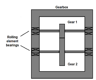
Figure 2: A generic gear rotor bearing system

We consider a generic geared-rotor bearing system, shown in Fig. 2, consisting of a rigid gearbox containing a spur gear pair mounted on flexible shafts, supported by rolling element bearings. Such a model has been previously used in other works (Antoniadou et al.,, 2015; Kahraman and Singh,, 1991) and its reliability has been shown in Kahraman and Singh, (1991). We now introduce it briefly.

The vibration response of the gearbox model we consider can be modelled by the following dimensionless equation of motion (Antoniadou et al.,, 2015):

$$\ddot{x}(t)+2z\dot{x}(t)+K(t)B(x(t))=F_{m}+F_{te}(t)+F_{var}(t).$$ (16)

The coordinate $x(t)$ represents the difference between the dynamic transmission error and the static transmission error. The quantity $z$ is a dimensionless linear viscous dumping parameter. $F_{m}$ represents the mean force excitations, while $F_{te}$ and $F_{var}$ pertain to internal excitations related to the static transmission error and external excitations related to wind turbulence, respectively. The quantity $F_{var}$ is derived from the fluctuating component of external input torque that simulates the wind turbulence’s effect. The backlash is simulated by the function

$$B(x(t)):=\left\{\begin{array}[]{lr}x(t)-1,&\text{for }x(t)\geq 1\\ 0,&\text{for }-1<x(t)<1\\ x(t)+1,&\text{for }x(t)\leq-1\end{array}\right\},$$ (17)

while the time varying mesh stiffness is incorporated via the periodic function $K(t)$. For a more detailed explanation of the specific structure of the functions mentioned and, more in general, for a deeper understanding of the gearbox model, see Appendix A and Antoniadou et al., (2015); Kahraman and Singh, (1991). Note that, this is a very simple wind turbine gearbox model, e.g., it ignores the bearing vibrations and wind turbine gearboxes usually consist of three gear stages with one or two being planetary stages. According to Antoniadou et al., (2015), it is sufficient for studies such as ours, since “more gear stages in a vibration signal would mean more frequency components at different frequency bands. Damage at a specific gear stage would therefore be shown in the vibration signal associated with the meshing frequency and its harmonics of the gear stage examined.” What is important in Antoniadou et al., (2015) and in our study, is to investigate the influence of the varying load conditions on the vibration signals, which can be achieved.

4.2 Including damage and wind turbulence.

Damage simulation

The damage we consider in this work is the crack of a gear’s tooth that, like other types of tooth damage, causes a reduction in the gear’s stiffness. This phenomenon can be represented by a periodic magnitude change in the mesh stiffness function $K(t)$ (Stander and Heyns,, 2005). Thus, an amplitude change is periodically applied to the mesh stiffness function to simulate the cracked tooth. In the simulations used in this work, the crack of a gear’s tooth was modelled by decreasing the dimensionless mesh stiffness function by 13% of its nominal stiffness for 5 degrees of the shaft rotation, periodically, for every rotation of the damaged gear. Similar modelling was used in previous studies, see  Antoniadou et al., (2015); Mohamed et al., (2018) for a more detailed explanation. Recapturing results reported in Antoniadou et al., (2015), we notice that in the model we consider, one should expect damage features to be evident at high-frequency components of the simulation signals because it is in the harmonics of the meshing frequency of the damaged gear pair that damage features occur. This is a phenomenon that was also observed in the experimental data used in Antoniadou et al., (2015).

Wind turbulence’s simulation

The representation of the wind as a smooth flow is not realistic because it does not take into account all its irregular and stochastic fluctuations. Due to wind turbulence, wind turbines experience transient and time-varying load conditions. In order to build a realistic model, we need to be able to consider and simulate these phenomena. To do that, it is possible to use a series of wind turbine aerodynamics codes, developed by the National Renewable Energy Laboratory (NREL, US) (Bir,, 2005). Specifically, the FAST design code has been used to simulate the turbulent wind conditions, associated with wind speed of 5 m/s and 13 m/s. See Appendix A for a deeper understanding of how the different wind conditions have been simulated.

4.3 Numerical data

The vibration response’s simulation of the gearbox model we considered in the previous section is given by numerical approximation of the function $\ddot{x}(t)$ obtained from the numerical solution of the dimensionless equation of motion (16) (Antoniadou et al.,, 2015; Kahraman and Singh,, 1991; Mohamed et al.,, 2018). The numerical solution of equation (16) has been computed with the MATLAB $ode45$ differential equation solver, with a fixed time step of 0.015. We originally intended to reproduce and use the simulated scenario as given in Antoniadou et al., (2015). Unfortunately, the data are not publicly available and could not be provided. Moreover, using their stated model’s parameters we could not obtain similar signals to those illustrated in that work. Thus, we choose the model parameters as to get data of at least qualitatively similar behavior. The details on how the numerical model has been built are described in Appendix A, where also all the parameters used for the simulations are reported in Table 3. The MATLAB code to perform the simulations will be made available after acceptance of the article and is in the supplementary material of the submission.

Simulations can represent different scenarios. On the one hand, we can produce numerical signals where the fluctuations of the input torque, due to wind turbulence, are not taken into account, i.e., $F_{var}(t)=0$ (Fig. 3). These simulations represent an improbable scenario in which the load on the wind turbine blades is constant. Such signals can be helpful to test different numerical strategies in a simplified context, and we will refer to them as signals in steady load conditions.

(a) undamaged case

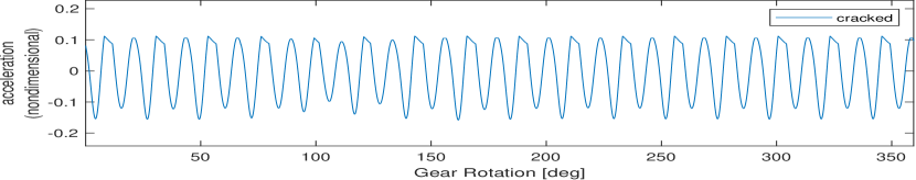
(b) damaged case

Figure 3: Simulation of an acceleration signal under a steady load condition

On the other hand, we can produce simulations representing the more realistic scenario where the wind is not considered as a uniform constant flow and its stochastic behaviour is included in the model. These simulations represent a situation in which the load on the wind turbine blades fluctuates and has a stochastic behaviour that determines random variations in the input torque. We will say that simulations generated in this scenario have varying load conditions. Fig. 4 and Fig. 5 show the acceleration signals of simulations with varying load conditions produced considering two different wind speeds.

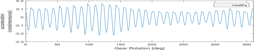
(a) undamaged case

(b) damaged case

Figure 4: Simulation of an acceleration signal under varying load condition with wind speed 5 m/s

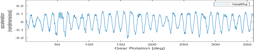
(a) undamaged case

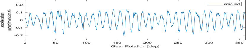
(b) damaged case

Figure 5: Simulation of an acceleration signal under varying load condition with wind speed 13 m/s

Independently of the scenario we consider, with steady or varying load conditions, we can produce signals representing a situation in which a perfectly healthy gearbox is modelled (Fig. 3(a),  4(a), 5(a)) or we can simulate a situation in which one of the gears is damaged (Fig. 3(b), 4(b), 5(b)). The simulated damage consists of a cracked tooth in one of the two gears. Recapturing some results from Antoniadou et al., (2015), we notice the signals simulated taking into account the wind turbulence are less smooth and show a more chaotic behaviour than the signals where the load condition is steady. This is motivated by the fact that when wind turbulence is incorporated into the model it introduces a stochastic component that perturbs the acceleration signals. The higher the simulated wind condition, the noisier the signal. Note that, independently of the wind condition considered, the damaged and healthy signals do not show any relevant difference and look almost identical. This is because only high-frequency components are affected by damage and just for a short time. This fact underlines that it would be very difficult to address the damage identification task without relying on a method that can extract only the relevant information from the signals.

5 Results

5.1 Results with simulation data

In this section, we study the numerical strategy for early damage detection based on multi-resolution dynamic mode decomposition proposed in Section 3. We compare our method with classical approaches used in this context, Fast Fourier transform as a frequency-domain approach, Time Synchronous Averaging (TSA) and EMD as a time-domain approaches.

Dataset

We analyze the vibration response data of the gearbox from three gear revolutions. We use the same two different health conditions of healthy and with cracked tooth and the same two wind speeds of 5 m/s (Fig. 6) and 13 m/s (Fig. 7) from before. The simulated signals are composed of 40201 one-dimensional snapshots. In the simulations that include the damage, the presence of the cracked tooth affects the signals once per rotation at $67^{\circ}$, $427^{\circ}$ and $787^{\circ}$. Note that we will make the simulated data and the code for generating the data available after acceptance of the article, it is part of the supplementary material of the submission.

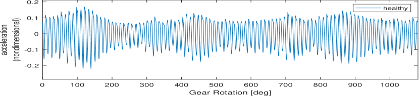
(a) undamaged case

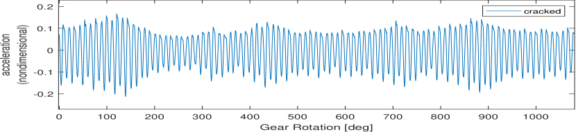
(b) damaged case

Figure 6: Simulation of an acceleration signal for three gear rotations under varying load condition with wind speed 5 m/s

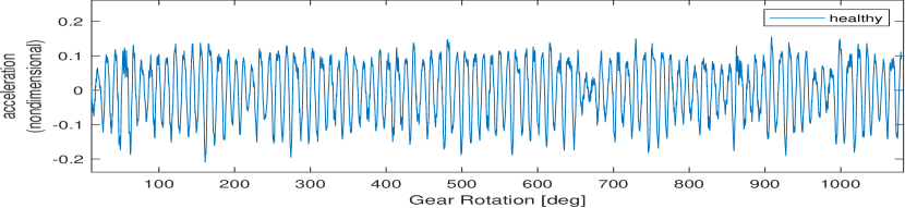
(a) undamaged case

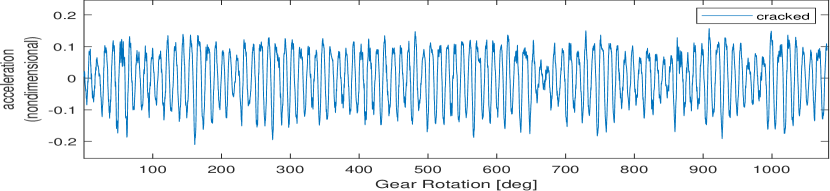
(b) damaged case

Figure 7: Simulation of an acceleration signal for three gear rotations under varying load condition with wind speed 13 m/s

5.1.1 Benchmark methods

Fast Fourier transform (FFT)

We now apply the FFT (Rao et al.,, 2011) to the vibration signals shown in Fig. 6 and Fig. 7. Fig. 8(a) and Fig. 8(b) show the Fourier spectra of the acceleration signals we have considered, representing the damaged and undamaged scenarios in varying load conditions associated with wind speed 5 m/s and 13 m/s, respectively. Independently of the wind condition considered, the differences between the healthy and cracked cases are very hard to identify just looking at the signals’ spectra. To be more specific, in Fig. 8(a) and Fig. 8(b) we highlight the meshing frequency and its harmonics, which are damage indicators because they relate to the frequency at which the damaged tooth has been excited (Li et al.,, 2019). Unfortunately, also in the highlighted frequencies, there is no significant or obvious magnitude change that allows us to identify the presence of damage.

This shows us an arduous difficulty that frequency methods have to overcome in this scenario: when the effects of the wind turbulence are included, it is very challenging to distinguish between the spectral characteristics of the signals associated with damage and those associated with wind turbulence. In addition to that, we have that due to wind turbulence, the spectra of the signals change randomly with time, making the damage identification task even more difficult. The shown results for the comparison between the healthy and damaged signals spectra are rather basic. But note, we do not aim to show that conventional gear monitoring techniques, for example Cepstrum or Kurtosis analysis, would be ineffective. These results mainly show that the operating conditions we are considering may have detrimental effects on the effectiveness of gear diagnostics techniques based on the signal’s spectral analysis.

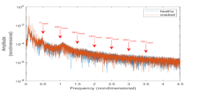
(a) wind speed 5 m/s

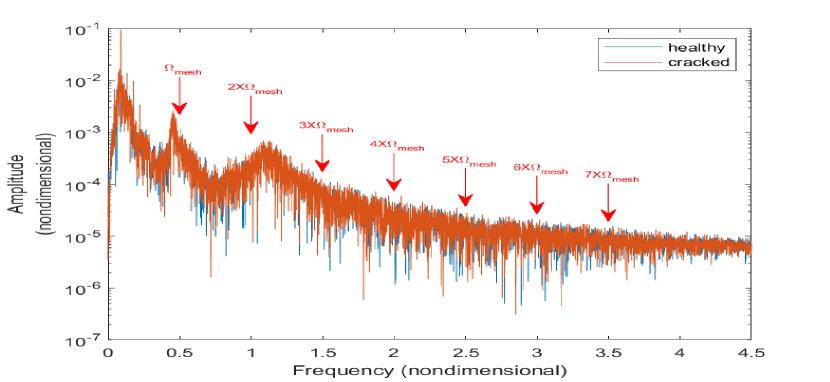
(b) wind speed 13 m/s

Figure 8: Fourier spectra of the dimensionless acceleration signals of the healthy and cracked tooth cases for varying load condition. The arrow-shaped cursors point to the mesh frequency, $\Omega_{mesh}$, and its harmonics.

Time Synchronous Averaging (TSA) and Hilbert transform (HT)

Time Synchronous Averaging (TSA) is a well-established procedure in rotating machines diagnostics (Randall,, 2021). One of the primary purposes of TSA analysis is to extract periodic waveforms from signals. For instance, it may be used to extract a periodic signal, such as the tooth meshing vibration of a single gear, from the whole machine’s vibration in order to detect damages by analyzing only the extracted signal’s component. Following along McFadden, (1986), we use TSA to demodulate the signals component associated with the gear mesh. After that, we use the Hilbert transform to demodulate the extracted TSA signal in order to detect local variations caused by damage and not visible to the eye. See McFadden, (1986), for a more detailed description of the TSA-based strategy we are going to review

Time Synchronous Averaging (TSA)

Given a signal $y(t)\in\mathbb{R}$, its time synchronous average $y_{a}(t)$ is defined as

$$y_{a}(t)=\frac{1}{N}\sum_{n=0}^{N-1}y(t+nT_{r}),$$ (18)

where $N\in\mathbb{N}$ and $T_{r}$ is the so-called periodic time. Formula (18) can be written as the convolution of $y(t)$ with a sequence of $N$ delta functions displaced by integer multiples of the periodic time $T_{r}$, i.e.,

$$y_{a}(t)=c(t)*y(t),$$ (19)

with

$$c(t)=\frac{1}{N}\sum_{n=0}^{N-1}\delta(t+nT_{r}).$$ (20)

It can be show that the desired signal component can be demodulated through TSA if the distance between the multiples of the periodic time is equal to its period. The main reason behind this fact is that (18) is equivalent in the frequency domain to the multiplication of the Fourier transform of $y(t)$ by a comb filter, removing all the components which fall outside the fundamental and harmonic frequencies of the desired signal. For more details see McFadden, (1987).

Hilbert transform (HT)

The HT of a signal $y(t)$ is defined as

$$\hat{y}(t):=H[y(t)]=\frac{1}{\pi}\int_{-\infty}^{\infty}\frac{y(s)}{t-s}ds=y(t)\ast\frac{1}{\pi t},$$ (21)

where $\ast$ denotes the convolution operator. Given the HT of $y(t)$ we can define the analytic signal

$$z(t):=y(t)+i\hat{y}(t)=a(t)e^{i\theta(t)},$$ (22)

where $i:=\sqrt{-1}$ is the imaginary unit, $a(t):=\sqrt{y^{2}(t)+\hat{y}^{2}(t)}$ is the instantaneous amplitude and $\theta(t)=\arctan(\frac{\hat{y}(t)}{y(t)})$ is the instantaneous phase. The instantaneous frequency is defined as $\omega:=\frac{\theta}{dt}$. The HT does not change the domain of the variable. Indeed, the HT of a time-dependent signal is also a function of time. Given a signal $y(t)$, the combination of (24) and (22) yields

$$y(t)=Re\Bigg{\{}\sum_{k=1}^{N}a_{k}(t)e^{i\theta_{k}(t)}\Bigg{\}}+r_{N}(t),$$ (23)

where $a_{k}(t)$ and $\theta_{k}(t)$ are the instantaneous amplitude and phase of the $k$-th IMF, respectively. We compute the Hilbert Transform using the “scipy.signal.function” in python.

Application of a TSA-based Strategy

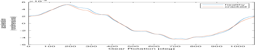
(a) TSA signal

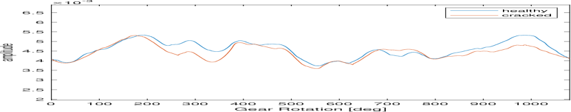
(b) Instantaneous amplitude

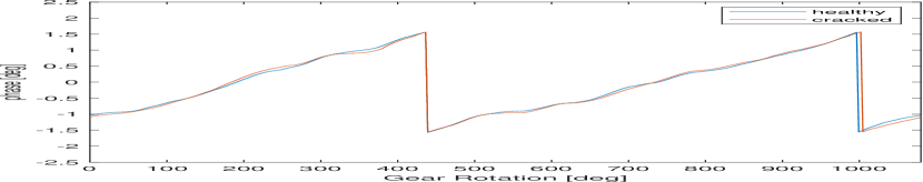
(c) Instantaneous phase

Figure 9: Results of TSA-based analysis, wind speed 5 m/s

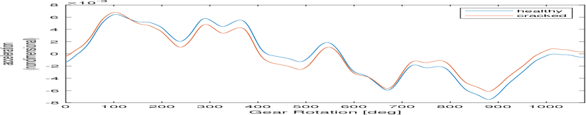
(a) TSA signal

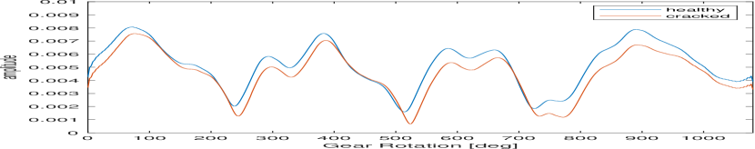
(b) Instantaneous amplitude

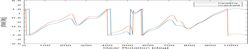
(c) Instantaneous phase

Figure 10: Results of TSA-based analysis, wind speed 13 m/s

Fig. 9(a) and Fig. 10(a) show the signals average obtained applying the TSA to acceleration signals in Fig. 6 and Fig. 7, respectively. Since, our aim was to use TSA to extract the vibration signal associated with the meshing frequency, we initially set $T_{r}=\frac{1}{\Omega_{mesh}}=2$, so that the distance between the multiples of the periodic time $T_{r}$ is equal to the meshing period. After that, we computed the instantaneous amplitude (Fig. 9(b) and 10(b)) and phase (Fig. 9(c) and 10(c)) of the TSA signals in order to detect small magnitude variations and highlight the presence of damage. As can be seen in Fig. figs. 9(b) to 9(c) and figs. 10(b) to 10(c), independently of the wind condition, both the instantaneous phase and amplitude associated with the healthy and cracked case show a very similar behavior. Thus, comparing the instantaneous phase and amplitude computed in the different health scenarios, we cannot emphasise any feature that indicates the presence of damage. The only exception is in Fig. 10(c), which shows that in the instantaneous phase associated with the cracked tooth, there is a sudden phase lag between $900^{\circ}$ and $1000^{\circ}$ of the gear rotation. Such a phase lag marks a substantial difference between the phase associated with healthy and cracked health conditions, and may be considered a damage indicator. However, Fig. 10(c) shows us that phase lags also arise in the instantaneous phase associated with the healthy signal and therefore may be misleading to consider only them as damage indicators. Furthermore, shifting the analysis focus only on the instantaneous amplitude and phase associated with the cracked scenario, there is no particular anomaly arising at the angles at which the cracked tooth interacts with the other gear ($67^{\circ}$, $427^{\circ}$ and $787^{\circ}$) that provides us with evidence of damage.

Notice that, we performed the above TSA-based analysis also using different values for the periodic time $T_{r}$. Specifically, we set $T_{r}=\frac{1}{m\Omega}$ with $m\in\{1,2,\dots,10\}$, so that the distance between the multiples of the periodic time $T_{r}$ is equal to the periods of the meshing frequency and its harmonics. Unfortunately, independently of the parameter choice, the results were qualitatively similar to those attained by setting $T_{r}=\frac{1}{\Omega_{mesh}}=2$. For the TSA approach we used the MATLAB function “tsa”, which sets automatically the parameter $N$ in (18) as the maximal amount of meshing periods in the time-span considered to analyze the signal.

In this work, we investigated TSA in combination with the HT, but there are other TSA-based techniques (Randall,, 2021), relying for example on Kurtosis analysis instead of the HT, which might give different results. Here we mainly want to show that TSA as other classical approaches may not always be effective in the operating conditions we are considering.

Empirical mode decomposition (EMD) and Hilbert transform (HT)

The EMD-based strategy we present here, consists of applying EMD together with HT to detect damages, and was introduced in the wind turbine damage detection context to overcome issues experienced by studying the signals’ spectral characteristics. See Antoniadou et al., (2015) for a more exhaustive analysis of the EMD-based fault detection method we are going to review.

Empirical mode decomposition (EMD)

The essence of EMD is to decompose the signal into oscillatory functions, also called intrinsic mode functions (IMFs). Each IMF represents characteristics of the signal associated with a certain frequency band and are such that

$$y(t)=\sum_{k=1}^{N}C_{k}(t)+r_{N}(t),$$ (24)

where $y(t)\in\mathbb{R}$ is a given sensor signal, $C_{k}(t)$ is the $k$-th IMF and $r_{N}(t)$ is the rest of the approximation performed by the IMFs. To identify the desired information in the IMFs there is not a principled approach, but it is important to know that the first IMFs represent structures in the signal associated with the highest frequencies, and the ones that come after depict lower frequency components (Huang et al.,, 1998). Generally, the first IMFs contain damage indicators, because they represent the highest frequency structures in the signal, which are those affected by the damage we are considering. For further details of the EMD algorithm see Huang et al., (1998). We use the PyEMD python package for the following analysis.

Application of an EMD-based strategy

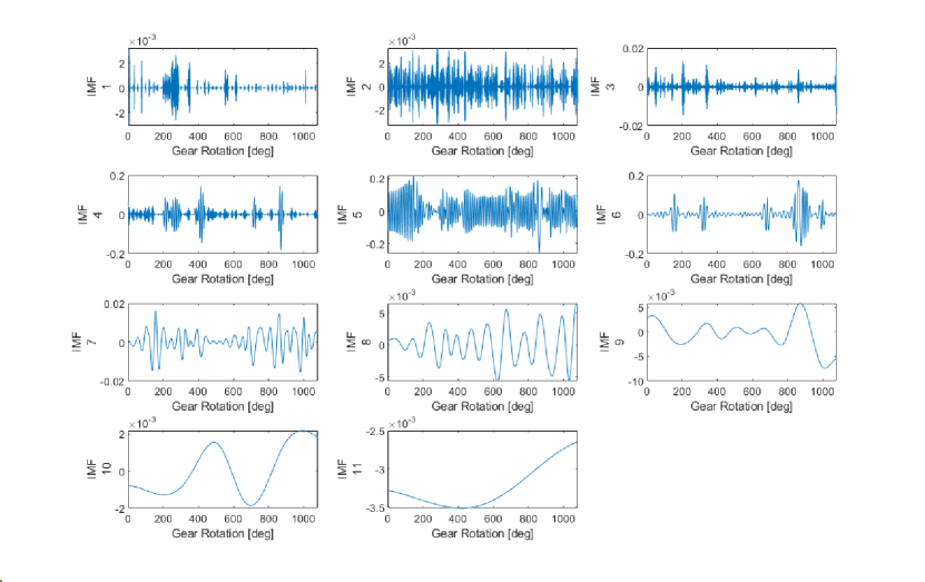
(a) undamaged case

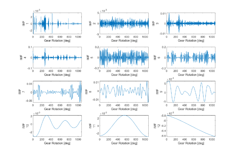
(b) damaged case

Figure 11: Intrinsic mode functions of simulations under varying load condition with wind speed 5 m/s

Fig. 11 represents the IMFs obtained applying EMD on the simulated vibration signals in Fig. 6. The signals in Fig. 6 represent the vibration response of the modelled gearbox under varying load condition associated with a wind speed of 5 m/s.

Looking at the IMFs in Fig. 11 one can observe that in the damaged case EMD has produced more IMFs than in the healthy case. This happens because EMD perceived the effects of damage as more signal components, and therefore it added IMFs to represent them. Another explanation is that the additional IMF is related to the mode mixing problem: some IMFs include damage features that are probably already contained in another IMF.

Analyzing the IMFs in more detail, it can be seen that the IMF 1 in Fig. 11(b) contains damage features. The damage features appear as increases in magnitude or pulses in the IMF, arising at the angles in which the cracked tooth affects the signal. Looking at the instantaneous amplitude of the first IMF (Fig. 12), it can be clearly seen that at the degrees where the cracked tooth interacts with the other gear, there are sudden increases of magnitude. Such increases of magnitude allow us to identify the presence of damage and, therefore, to perform the damage identification task. Unfortunately, from Fig. 12, it is also clear that together with those related to damage, there are other pulses in the IMF 1, probably related to the varying wind condition, which make the identification of damage features a very challenging task. In particular, without previous knowledge about where the cracked tooth affected the signal, we would not have been able to identify it. A possible explanation for such an event is that the mode mixing problem occurred. Thus, information related to the frequency bands affected by damage and by wind turbulence is represented in the same IMF and can not be distinguished trivially. As a consequence of the mode mixing problem, we could also have that different IMFs contain the same frequency band information. For instance, using acceleration signals representing a scenario related to those we consider in this work, we found that sudden increases of magnitude caused by a cracked tooth could be identified in different IMFs. Thus, information related to the frequency band affected by the damage was contained in different IMFs. Such a problem was also experienced in Antoniadou et al., (2015), where they use EMD to study signals similar to those analyzed here.

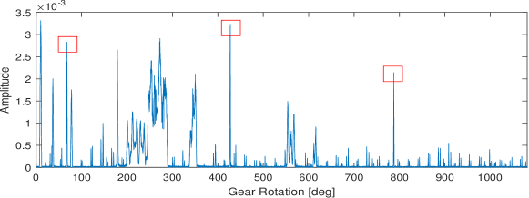
Figure 12: Instantaneous amplitude of IMF 1 computed in the damaged case with wind condition 5 m/s. The pulses related to the presence of damage are marked with red squares

Analyzing the simulated data generated with the higher wind speed of 13 m/s we could not successfully perform the damage identification task. Specifically, applying EMD to signals in Fig. 7(b), no IMFs could visually highlight the different nature of the effects of the wind and of the damage on the signal.

After this brief analysis, it is clear that one of the disadvantages of EMD is that information about the damage’s effects in the signal is not localized: EMD does not tell us which frequency-band each IMF exactly represents. Thus, we do not know in which IMF damage features can be detected. The second main weakness of EMD is the mode mixing problem, which affects the interpretability of the method and its capability to perform the fault detection task effectively. As we will see, the numerical procedure we propose overcomes these problems thanks to the characteristics of the mrDMD algorithm.

5.1.2 mrDMD-based approach for damage detection

For our numerical experiments with mrDMD, we use the simulated gearbox vibration signals shown in Fig. 6 and Fig. 7 that represent the vibration response of the modelled gearbox in the damaged and undamaged scenarios under the two different wind conditions we are considering. The same data was used to test the EMD-based method previously. The length of the delay $d$ has been fixed to $d=32000$. Thus, looking at the residual $\mathbf{r}_{0}$ we are analysing a portion of the signal representing its temporal evolution for $860^{\circ}$ of the shaft rotation. The number of the decomposition levels $L$ in the mrDMD algorithm has been set to $L=11$. We use the PyDMD python package, where we use the previously mentioned threshold strategy for the choice of parameters.

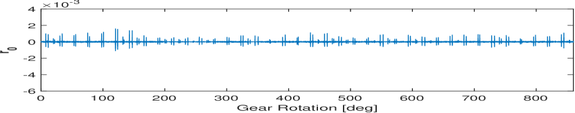
(a) undamaged case

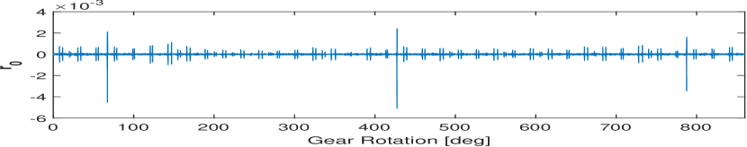
(b) damaged case

Figure 13: Residual of a simulation under varying load conditions with wind speed 5 m/s, computed calculating $L=11$ decomposition levels

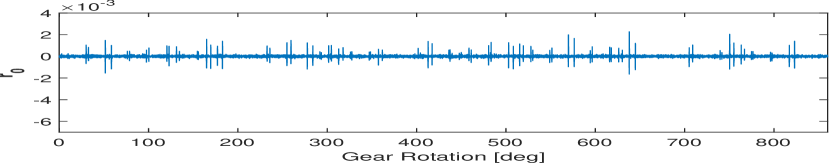
(a) undamaged case

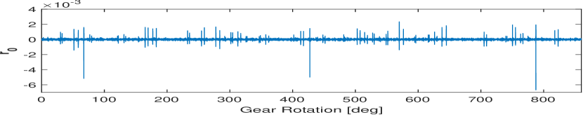
(b) damaged case

Figure 14: Residual of a simulation under varying load conditions with wind speed 13 m/s, computed calculating $L=11$ decomposition levels

MrDMD-residual analysis on simulation data

Fig. 13 and Fig. 14 represent the results of the mrDMD-based approach that we proposed in Section 3. The first observation we make, comparing the residuals obtained from simulations produced with different wind conditions in the undamaged case (Fig.  13(a), 14(a)), is that when the wind speed is higher the high-frequency signals’ structures represented by the residuals show a more irregular behaviour. This is because high-frequency structures are affected by wind turbulence, which is more relevant and volatile for higher wind speed conditions. The second observation concerns simulations representing the damaged and undamaged cases in the different wind conditions. Considering only the residual $\mathbf{r}_{0}$, the effects of the damaged tooth are clearly visible as sudden increases in magnitude arising at the angles in which the cracked tooth affects the signal (Fig. 13(b), 14(b)). The effects of the cracked tooth on the residuals can be further analyzed by considering their instantaneous amplitudes (Fig. 15 and Fig.  16) computed through the Hilbert transform. Independently of the wind condition considered and the residuals’ mean breadth, looking at the instantaneous amplitudes, the different characteristics of the residuals associated with the damaged and undamaged cases are even more evident. The instantaneous amplitudes related to both the healthy and damaged scenarios present a spiky structure. However, in the undamaged cases (Fig.  15(a), 16(a)), the spikes are of similar magnitude over the time-span analyzed, while in damaged scenarios (Fig.  15(b), 16(b)), the magnitudes of the spikes are much higher at the angles in which the cracked tooth affects the signal, making the damage identification even easier than it was considering only the residuals.

It can be clearly seen that the numerical procedure we propose can be effectively employed to highlight the effects of the cracked tooth on the signal, distinguishing them from the effects of the varying load condition, and enabling us to identify the damage independently of the wind condition. Moreover, a consistent advantage of the proposed strategy with respect to EMD is that the information related to damage is localized. With the proposed strategy, all the information required is contained in the residual. Note that, due to the mode mixing problem, such a residual strategy is not feasible with EMD. To effectively employ EMD to detect damages, a user search among the produced IMFs is needed to identify those structures containing information related to damage.

We note that we also applied our procedure on signal simulated with parameters other than those represented in Table 3. Specifically, we considered two additional internal excitation parameter settings and two crack lengths in the numerical model. In addition to that, we performed each experiment in each of the two wind conditions we considered so far. Overall, we performed experiments in eighteen operating conditions, which gave results comparable to those here presented. The specific parameter settings are given in Appendix A.

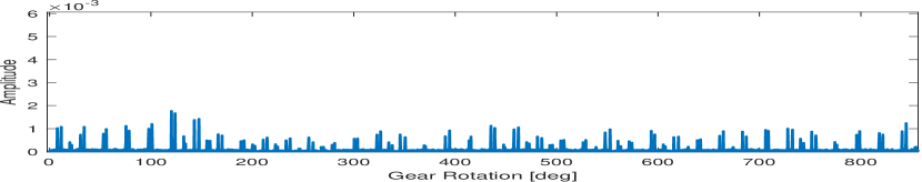
(a) undamaged case

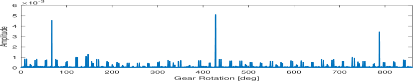
(b) damaged case

Figure 15: Instantaneous amplitude of residual $\mathbf{r}_{0}$ ($L=11$), wind speed 5 m/s

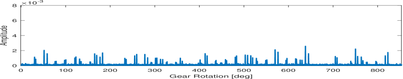
(a) undamaged case

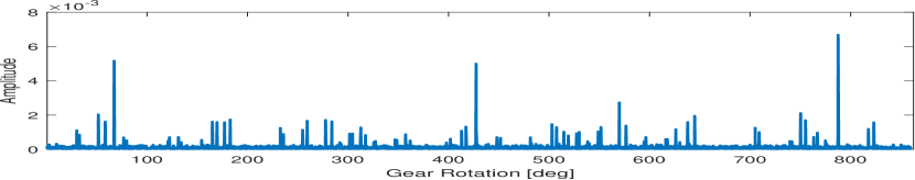
(b) damaged case

Figure 16: Instantaneous amplitude of residual $\mathbf{r}_{0}$ ($L=11$), wind speed 13 m/s

We remark that the choice of the number of decomposition levels $L$ to compute strongly affects the effectiveness of our analysis. Specifically, if the number of calculated decomposition levels is not high enough, the residual would consist of structures associated with a frequency band that would also include those low-frequencies not affected by the damage. As we will see shortly, the presence of the cracked tooth has a negligible effect on the structures associated with lower frequencies. Therefore, the residual would also consist of components that do not provide any meaningful insight for the damage identification process, which would dilute the valuable information. Consequently, the residual would not be able to highlight the presence of damage. To observe such a phenomenon, see Fig. 17, which represents the residuals computed applying the proposed procedure on vibration signals in Fig. 7 associated with wind speed 13 m/s, considering a delay $d=32000$ and calculating $L=7$ decomposition levels. It can be clearly seen that, in this case, $L=7$ decomposition levels are not enough to encode in the residual only the relevant information associated with the highest frequencies and related to damage. There is no obvious difference between the two residuals in Fig. 17. Thus, they can not be employed to perform damage detection.

To correctly choose the number of decomposition levels to compute and successfully apply the proposed procedure for damage detection, we need information about the frequencies affected by the damage we want to identify. Fortunately, in condition monitoring, the damage we want to identify and the frequencies affected by it can often be assumed to be known (Antoniadou et al.,, 2015).

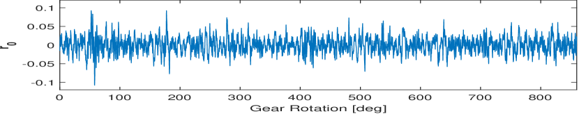
(a) undamaged case

(b) damaged case

Figure 17: Residual of a simulation under varying load conditions with wind speed 13 m/s, computed calculating $L=7$ decomposition levels. Using these lower frequencies the damage cannot be detected.

Modal analysis with mrDMD on simulation data

We now investigate more closely the modes’ properties and how the proposed procedure works. To this aim, we analyze the modes computed via mrDMD, calculating $L=11$ decomposition levels, and used to obtain the residuals $\mathbf{r}_{0}$ in Fig. 14. We mainly focus on the scenario associated with the wind speed of 13 m/s because signals generated employing the same gearbox model we use and considering a similar wind condition were already simulated and studied in Antoniadou et al., (2015). Thus, we can exploit the knowledge developed there about the signals’ physical characteristics to better interpret and understand the properties of the modes generated by mrDMD.

Recall that we can compute the residual $\mathbf{r}_{0}$ associated with a signal by subtracting from the first time-delay snapshot, $\mathbf{\tilde{y}}(t_{0})$, its mrDMD approximation $\mathbf{\hat{y}}(t_{0})$, i.e., $\mathbf{r}_{0}=\mathbf{\tilde{y}}(t_{0})-\mathbf{\hat{y}}(t_{0})$. According to (12), if we set $t_{0}=0$, the mrDMD approximations of the first time-delay snapshots can be explicitly written as

$$\mathbf{\hat{y}}(t_{0})=\sum_{l=1}^{L}\sum_{k=1}^{m_{L}}b_{k}^{(l,1)}\boldsymbol{\phi}_{k}^{(l,1)}.$$ (25)

Specifically, the linear combination of the modes $\phi_{k}^{(l,1)}$, computed at the first time bin of each decomposition level, gives the mrDMD approximation of the first time-delay snapshot representing the evolution of the analyzed signal for a time-span as large as the delay. It is important to notice that to obtain the residuals $\mathbf{r}_{0}$ only the modes computed at the first time bin of each decomposition level are needed, and that each one of the modes $\boldsymbol{\phi}_{k}^{(l,1)}$ is associated with a frequency $\omega_{k}^{(l,1)}$.

In the scenario associated with wind speed 13 m/s, we know that the wind turbulence mainly affects the signal at its highest frequencies, as it was observed in Antoniadou et al., (2015) for the similar wind speed of 12 m/s.

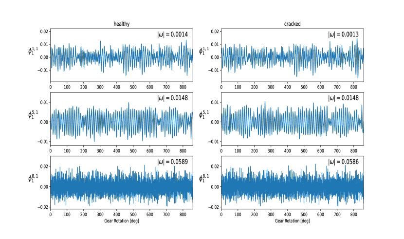
Figure 18: First modes computed at the first time bins of the decomposition levels $l=1,5,8$ obtained applying the proposed analysis on simulation under varying load conditions with wind speed 13 m/s and calculating $L=11$ decomposition levels

Fig. 18 depicts 3 of those modes used to compute the reconstructed time-delay snapshots $\mathbf{\hat{y}}_{0}$ required to obtain the residuals $\mathbf{r}_{0}$ in Fig. 14. The modes in Fig. 18 have been computed applying the proposed analysis on vibration signal associated with wind speed 13 m/s in the healthy and damaged scenario (Fig. 7). Specifically, they are the first modes computed at the first time bins of the decomposition levels $l=1,5,8$. Looking at Fig. 18, we can make a number of observations that give us a better understanding of the modes’ properties and that generally hold for modes computed at different time bins and decomposition levels. Analyzing Fig. 18, it is clear that the higher the decomposition level, the higher is the energy content $|\omega|$ associated with the modes computed in it. Here $\omega$ is the frequency defined in Algorithm 1. This fact is empirical proof of what we already saw from a theoretical perspective in Section 3, where the mrDMD has been explained, and such a property of the modes was already introduced. Another consideration is that modes computed at the highest decomposition level are much noisier than those calculated at lower levels. This can be explained by the fact that high-energy modes incorporate the effects of the wind turbulence on the signal, which as we know from Antoniadou et al., (2015) are more evident at high-frequencies. Thus, it further confirms that high-energy modes contain structures associated with high-frequencies, and that the residuals consist of those structures associated with the highest frequencies. Finally, we observe that in Fig. 18 the modes computed in the healthy scenario and their associated energies ($|\omega|$) are qualitatively the same as those calculated from signals that include the damage. This, can be motivated by the fact that the modes depicted are associated with frequencies not affected by the presence of the cracked tooth. More in general, we found that in this scenario, the effects of damage can be effectively identified and discerned from those related to wind turbulence only in those structures associated with the highest frequencies.

Automation

An advantage of the procedure we propose, compared to EMD, is that it may allow the automation of the damage detection process. The main reason for that is that it localizes the information related to damage.

Considering how EMD works, here, after a certain number of IMFs have been produced, a user made choice has to be performed to pick out all those IMFs that may contain damage features, and therefore need to be further analyzed. In general, we know that information related to the damage we are considering should be in the first IMFs, which are those associated with higher frequencies in the signal. However, this is only a rule of thumb, and because of the mode mixing problem, there is no principled way to perform the IMFs’ choice. Therefore, using EMD, there is no obvious method to automatize the damage identification process.

On the contrary, the procedure we propose localizes the information related to damage in the residual. Thus, there is no need for a modes’ selection, and the cracked tooth detection task reduces to identifying sudden increases of magnitude and anomalies within the residual. A broad spectrum of peak detection methodologies is available and should be applicable to automatize the damage identification process (Du et al.,, 2006; Harmer et al.,, 2008; Jordanov and Hall,, 2002). Automatizing the damage identification process would be very advantageous in practice because it would allow to monitor the health condition of several gearboxes simultaneously and continuously, but it is out of the scope of this paper.

5.2 Results with experimental data

There is a lack of real or experimental data for the considered damage scenario under the presence of wind fluctuations. Instead, we now consider experimental data under controlled operating situations that offer other non-trivial challenges than the previously studied simulation data. Specifically, in the experimental data, the acceleration signals are mixed with other signals from different interacting gearbox components and are significantly attenuated by the dynamics of the case and other elements in the transmission path. Note that with the results on this experimental data, we want to show that the proposed mrDMD approach can overcome these additional challenging effects. We do not claim that for these controlled operating situations, our method can detect damages more effectively than other gear diagnostic techniques.

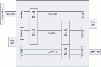
Figure 19: Schematic of the gearbox (PHMSociety,, 2009)

Table 1: Geometry double stage reduction gearbox with spur gears set-up and its operating conditions

Geometry			Operating conditions (angular speed)
components	Spur gear		1st-HL	2nd-HL	3rd-LL	4th-HL	5th-LL
Input shaft: 1-Input Pinion	32 teeth		30 Hz	35 Hz	40 Hz	45 Hz	50 Hz
Idler shaft: 1st idler gear	96 teeth		10 Hz	11.7 Hz	13.3 Hz	15 Hz	16.7 Hz
Idler shaft: 2nd (output) idler gear	48 teeth		10 Hz	11.7 Hz	13.33 Hz	15 Hz	16.7 Hz
Output shaft: output pinion	80 teeth		6 Hz	7 Hz	8 Hz	9 Hz	10 Hz
HL = High load condition; LL = Low load condition

Table 2: Health conditions of the double stage reduction gearbox with spur gears set-up

health condition

Gears

Bearings

Shaft

(file name)

32T

96T

48T

80T

IS:Is

ID:Is

OS:Is

IS:Os

ID:Os

OS:Os

Input

Output

Healthy (Spur 1)

Good

Good

Good

Good

Good

Good

Good

Good

Good

Good

Good

Good

Broken tooth (Spur 4)

Good

Good

Eccentric

Broken

Ball

Good

Good

Good

Good

Good

Good

Good

ID = Idler shaft; IS = Input shaft; Is = Input side; OS = Output shaft; Os = Output side; T = teeth

Experimental dataset

We consider accelerations signals from the double stage reduction gearbox described in PHMSociety, (2009) and shown in Fig.  19. Data were sampled synchronously from accelerometers mounted on both the input and output shaft retaining plates, and were collected at 30, 35, 40, 45 and 50 Hz input shaft speed, under high and low loading. The sampling frequency is set to 66666.67 Hz and the acquisition time is 4 seconds. Additionally, the runs were repeated twice for each load and speed. Both spur and helical gears are used separately in the setup of the gearbox to obtain different datasets.

In this initial study, we analyze the data from the accelerometer mounted on the output shaft retaining plate of the spur gearbox. To demonstrate our method’s capability of detecting signs of damage, we compare how it operates under five different operating conditions given by different input shaft speeds and loading. The geometry of the gearbox and the operating conditions we consider are summarized in Table 1. As can be seen in Table 2, we consider two different health conditions. Either all the components of the gearbox are healthy, or there is a broken tooth together with an eccentric gear and a damaged bearing’s ball in the input shaft.

Fig. 20 shows representative acceleration signals, from the experimental dataset, generated with different load and speed conditions. Comparing the acceleration signals in the damaged and undamaged cases, the damage effects are plainly visible as sudden periodical magnitude increases in the signals. This is a characteristic shared by all the acceleration signals we analyze, independently of the operational condition considered. Notice that, the x-axis in Fig. 20 are labeled with time and not degrees of rotation as previously done with simulation data. This is because in the damaged scenarios the eccentric gear on the Idler shaft’s output side may modulate the speed of the gear on the output shaft (Mba et al.,, 2017), which is the one with the broken tooth. Consequently, in the damaged scenario, the actual angular speed of the gear on the output shaft may differ from the theoretical angular speed reported in Table 1. Since we do not know the entity of the damage it is not possible to determine a priori degrees of rotation of the output gear for a fixed time interval.

For each operating condition we analyse, we consider a portion of the signal associated with three rotations of the output shaft in healthy condition plus the following 15000 snapshots. This will ensure that when we apply our method with a time delay embedding associated with three rotations of the healthy output shaft we have 15000 available time-delay snapshots in each scenario we consider.

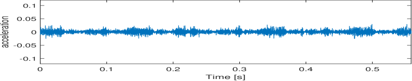
(a) undamaged case

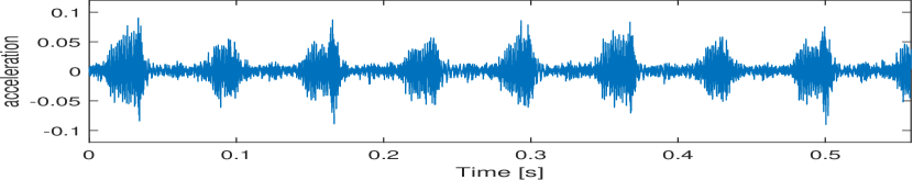
(b) damaged case

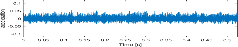
(c) undamaged case

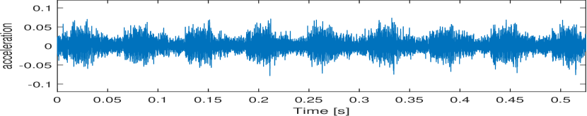
(d) damaged case

Figure 20: Acceleration signals from the double stage reduction gearbox with spur gears set-up operating at different conditions. (a) and (b) 45Hz input shaft speed with high load. (b) and (c) 50Hz input shaft speed with low load

5.2.1 mrDMD-based approach for damage detection on experimental data

We now apply the proposed procedure to acceleration signals from the double stage reduction gearbox with spur gears set-up operating at 30, 35, 40, 45 and 50 Hz input shaft speed, under high and low loading. Our goal is to show that the anomalies caused by the broken tooth and other damages, that affect high frequency structures of the signal, can be detected by analyzing the residuals even in a scenario in which the acceleration measurements include the dynamics of the case and other elements in the transmission path. In each operating condition we compute $L=8$ decomposition levels, and consider a delay $d$ associated with three rotations of the healthy output shaft. Thus, looking at the residuals instantaneous amplitudes, we are analyzing a portion of the signal representing its temporal evolution for the time needed from the healthy output shaft for a rotation of $1080^{\circ}$. Since each operating condition has a different output shaft speed, the delay $d$ will be given by different amounts of snapshots. The parameter choices have been summarized in Appendix B, Table 5.

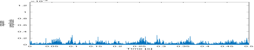
(a) undamaged case

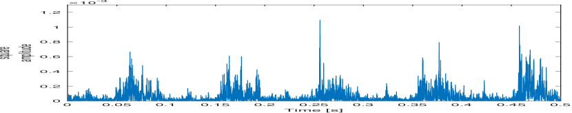
(b) damaged case

Figure 21: Square instantaneous amplitudes of the residuals $\mathbf{r}_{0}$ (L=8) obtained from acceleration signals from the double stage reduction gearbox with spur gears set-up operating at 30Hz input shaft speed with high load

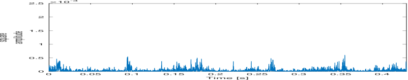
(a) undamaged case

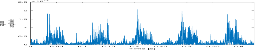
(b) damaged case

Figure 22: Square instantaneous amplitudes of the residuals $\mathbf{r}_{0}$ (L=8) obtained from acceleration signals from the double stage reduction gearbox with spur gears set-up operating at 35Hz input shaft speed with high load

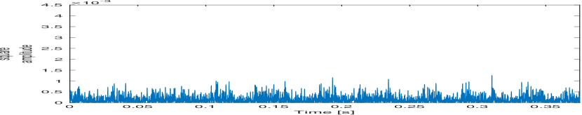
(a) undamaged case

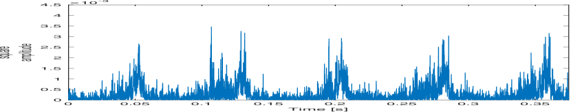
(b) damaged case

Figure 23: Square instantaneous amplitudes of the residuals $\mathbf{r}_{0}$ (L=8) obtained from acceleration signals from the double stage reduction gearbox with spur gears set-up operating at 40Hz input shaft speed with low load

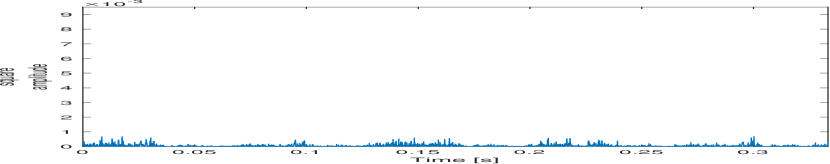
(a) undamaged case

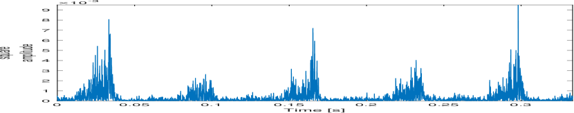
(b) damaged case

Figure 24: Square instantaneous amplitudes of the residuals $\mathbf{r}_{0}$ (L=8) obtained from acceleration signals from the double stage reduction gearbox with spur gears set-up operating at 45Hz input shaft speed with high load

MrDMD-residual analysis on Experimental data

Fig. 21-25 represent the results of the mrDMD-based approach on the experimental data. Specifically, they show the square instantaneous amplitudes of the residuals obtained by applying the proposed procedure to acceleration signals operating at 30, 35, 40, 45 and 50 Hz input shaft speed, under high and low loading.

As we have previously seen, independently of the operational condition, in the acceleration signal associated with the damaged scenario, the damage effects are visible as sudden periodical magnitude increases (Fig. 20). Interestingly, such behavior is reflected in the high-frequency components of the signals represented by the residuals, as it can be seen by looking at their instantaneous amplitudes (Fig. 21-25). More precisely, comparing the residuals instantaneous amplitudes obtained in the damaged and undamaged scenarios in the different operating conditions the effects of damage can be clearly detected as periodical sudden increases of magnitude.

From the mrDMD analysis on simulation data, we would expect only three main increases of magnitude in the instantaneous amplitudes of the residual associated with the damaged cases. Specifically, we would expect the magnitude increases to arise when the broken tooth part of the output gear interacts with the gears mounted on the Idlers shaft. Notice that, the residuals instantaneous amplitudes associated with the damaged scenarios show more than three prominent magnitude increases. This can be motivated by the presence of the other damages. In particular, the eccentric gear in the Idler shaft’s output may modulate the speed of the gear on the output shaft, which is the one with the broken tooth. Consequently, the broken tooth part of the output gear interacts with the eccentric gear more than three times during the time-span we are considering, generating more magnitude increases.

Nevertheless, also in the more challenging scenario offered by the experimental data, the developed procedure can highlight the effects of damage on the signal’s high-frequency components, providing a tool that enables us to clearly distinguish the healthy scenarios from the damaged ones in various operating conditions.

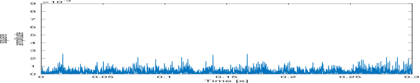
(a) undamaged case

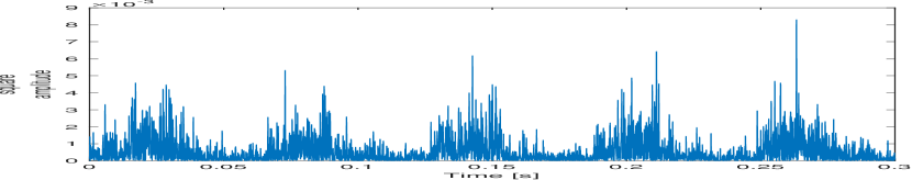
(b) damaged case

Figure 25: Square instantaneous amplitudes of the residuals $\mathbf{r}_{0}$ (L=8) obtained from acceleration signals from the double stage reduction gearbox with spur gears set-up operating at 50Hz input shaft speed with low load

Modal analysis with mrDMD on experimental data

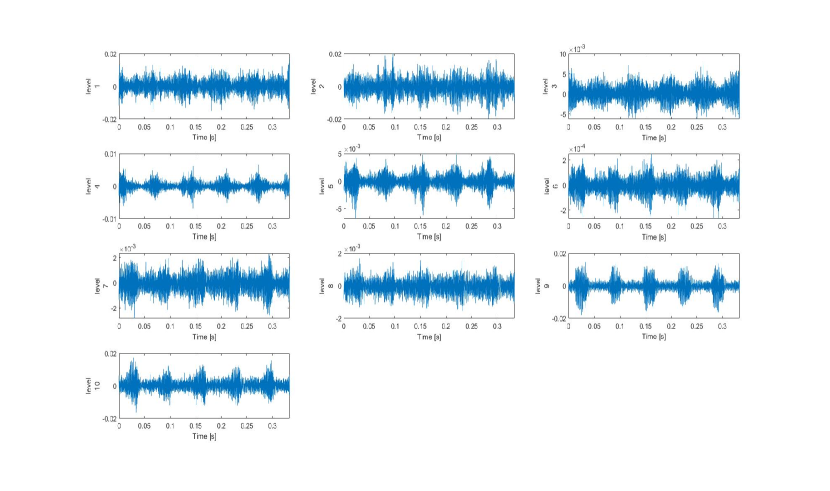
Figure 26: Signal components $\mathbf{p}_{0}^{l}$, $l=0,1,2,\dots,10$, computed from acceleration signal of double stage reduction gearbox with spur gears set-up operating at 45Hz input shaft speed with high load

For the simulated data we performed a modal analysis where we in particular investigated the first mode for several decomposition levels. Here, for additional insight, we instead consider at each level “ $l$ ” the signal’s reconstruction, $\mathbf{p}^{l}_{0}$ provided by the modes computed at that level, i.e.,

$$\mathbf{p}^{l}_{0}=\sum_{k=1}^{m_{l}}b_{k}^{(l,1)}\boldsymbol{\phi}_{k}^{(l,1)}.$$ (26)

The subscript “ 0 ” is due to the fact that we are assuming we want to analyze the first time-delay snapshot, the one computed at time $t_{0}$, as we did in the mrDMD-residual analysis. Consequently, we are interested in the modes computed in the first time-bin of each level.

Each signal component $\mathbf{p}^{l}_{0}$ summarizes information of the modes computed at level $l$. Note that, each mode is associated with a specific frequency. Therefore, each signal component $\mathbf{p}^{l}_{0}$ represents information related to a specific frequency band. Once the components $\mathbf{p}^{l}_{0}$ that highlight damage features have been identified, and the frequency band or the multiple frequency bands affected by damage have been assessed, one can focus only on the signal’s structures of interest, either through the residual or by considering the components $\mathbf{p}^{l}_{0}$ associated with the frequecy bands of interest.

Let us give an example. Fig. 26 illustrates ten components $\mathbf{p}^{l}_{0}$, $l=0,1,\dots,10,$ obtained applying the mrDMD approach we propose to the acceleration signal in Fig. 20(b) generated in high load conditions at 45hz input shaft speed. The delay embedding $d$ is the same we previously considered. In the scenario we are considering, the first four signal components can be assumed to be mainly associated with the core part of the signal, and the effects that damages have on them are negligible. Thus, the relevant signal components for our analysis are those computed at higher decomposition levels. It can be seen that the characteristics of the last two signal components are very different from the previous ones. In particular, both the components computed at the eighth and the ninth decomposition level show a much more prominent spiky behaviour than the previous ones, and the magnitude of the spikes is higher as well. Moreover, after the eighth level of decomposition, there is a sudden increase in the magnitude of the computed signal components. These two factors lead us to conclude that the signal components computed at the eighth and ninth decomposition levels are associated with features related to damage. To provide additional evidence, we analyze the signal reconstruction, $\mathbf{y}_{0}^{1-8}$ (Fig. 27), obtained using the components computed at the first eight levels, it can be seen that the sudden increases of magnitude that characterize the presence of damage in the original acceleration signal (Fig. 20(b)) are not represented. This shows us that the features related to damage are mainly highlighted in higher frequency structures, among which there are the structures represented by the eighth and ninth signal components, i.e., $\mathbf{p}^{9}_{0}$ and $\mathbf{p}^{10}_{0}$. Recall that we computed eight decomposition levels in our mrDMD-residual analysis on experimental data. Thus, the signal components $\mathbf{p}^{9}_{0}$, and $\mathbf{p}^{10}_{0}$, were included in the residual.

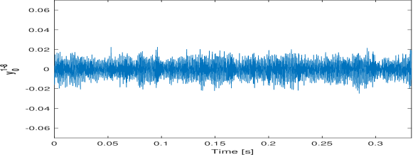
Figure 27: Partial reconstruction, $\mathbf{y}_{0}^{1-8}$, of acceleration signal from double stage reduction gearbox with spur gears set-up operating at 45Hz input shaft speed with high load. The partial reconstruction is obtained with the first eight signal components, i.e., $\mathbf{y}_{0}^{1-8}=\sum_{l=1}^{8}\mathbf{p}^{l}_{0}$

6 Conclusion

In this work, we proposed a numerical procedure for damage detection, which exploits DMD’s strengths of being equation-free and data-driven. From our results with simulation data, we observed that performing damage detection with Fourier analysis, TSA or EMD can be very challenging in a scenario that includes varying load conditions. We also saw that both, our mrDMD-based method and the EMD strategy, decompose the original signal into modes that can be used to extract characteristics of the signal associated with different frequencies. In particular, both methods can highlight those high-frequency structures affected by wind turbulence and change in stiffness caused by the cracked tooth and that can be effectively used to identify damages. On the one hand, we saw that the IMFs, produced by EMD, represent structures in the signal that are not associated with specific frequencies but rather with frequency bands. Moreover, the information contained in an IMF can be related to a too broad frequency band, or the same frequency information can be contained in different IMFs. These facts affect the interpretability of the IMFs and the effectiveness of EMD to perform fault detection because the information related to damage is not localized. On the other hand, mrDMD associates each mode with a specific frequency. Exploiting this fact, the proposed numerical procedure was able to identify those structures in the signal where features related to damage were highlighted. In particular, differences in the residuals’ magnitude (Fig. 13 and Fig. 14) as well as in their instantaneous amplitude (Fig. 15 and Fig.  16), allowed the identification of the cracked tooth visually, independently of the wind condition considered. We also saw, from the results with experimental data, that while the proposed mrDMD-based strategy is influenced by accelerations signals affected by additional vibration sources, it still is a feasible approach for damage detection.

The first strength of the proposed analysis is that, as EMD, it does not consider the signals’ spectra, avoiding all the issues related to the non-deterministic time variation of the signals spectral properties caused by the varying load condition. The other advantage is that the mrDMD algorithm is not affected by the mode mixing problem, as it is for EMD-based strategies. Moreover, with the strategy here proposed, information related to the effects of the damage in the signal is localized in the residual.

Note that, the strategy we propose can be further improved to perform an effective analysis in more challenging scenarios. Specifically, several DMD improvements could be applied in the second step of Algorithm 2  (Héas and Herzet,, 2016; Hemati et al.,, 2017; Matsumoto and Indinger,, 2017). A particularly beneficial DMD improvement in this context was developed in Hemati et al., (2017). It consists of building unbiased and noise-aware DMD by explicitly accounting for noise in the signal. Such modification could allow our method to distinguish between the noise introduced by wind turbulence, transmission path vibrations and damage effects more easily. Furthermore, additional improvements can be introduced working on the indicator function in (11). In general, it is possible to introduce various functional forms for the indicator function that can be used advantageously. For instance, one could consider the indicator function to take the form of different wavelet bases i.e. Coiflet, Haar, Fejér-Korovkin, etc.

In conclusion, this work shows the potentialities of a DMD-based strategy to perform anomaly detection, analyzing simulated signals representing the vibration response of a gearbox under varying load condition and experimental data generated with various speed and load operating conditions. The results we reported here tell us that this DMD-based strategy promises to provide high quality results by overcoming spectral and mode mixing related problems in a scenario that includes the effects of wind turbulence. Further research on mrDMD in the context of fault detection and condition monitoring of wind turbines, and related machinery, is warranted.

Appendices

Appendix A

The aim is to build an equation of motion for the gearbox model considered in Section 4 that takes into account the rotational movements of the two gears. To do that, such an equation needs to include the two main factors that affect the gears’ movements, which are: the input torque that acts on the driving gear and the effects of the interaction between the teeth of the two gears. The area where the interaction between the two gears takes place is called gear mesh.

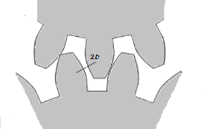
Figure 28: The backlash between gears

The Gear mesh

To include the effects of the interaction between the teeth of the two gears we include into the equation of motion we are going to build the backlash, the time-varying mesh stiffness function $\bar{K}(\bar{t})$, the static transmission error $\bar{e}(\bar{t})$, and a linear viscous dumping parameter $\bar{C}$. The backlash is a clearance or lost motion of the gears caused by gaps between the teeth (Fig. 28). This phenomenon is incorporated in the model via the backlash function $B(\bar{x}(\bar{t}))$, where $\bar{x}(\bar{t})$ is displacement function that will be introduced shortly. The time-varying mesh stiffness function, $\bar{K}(\bar{t})$, describes the varying stiffness of the teeth that are in the gear mesh, and is caused by the transition from single to double and double to single of pairs of teeth in contact. Finally, the static transmission error $\bar{e}(\bar{t})$, is caused by geometrical errors of the teeth profile and represents the difference between the actual position of the driven gear and the position it would occupy if the gears’ edges were manufactured perfectly. The mesh stiffness and static transmission error functions are assumed to be periodic functions of time and, in the theoretical setting we are considering, can be expressed in the following Fourier form:

$$\bar{K}(\bar{t})=\bar{K}\left(\bar{t}+\frac{2\pi}{\bar{\Omega}_{mesh}}\right)=\bar{K}_{m}-\sum_{j=1}^{\infty}\bar{K}_{j}\cos\left(j\bar{\Omega}_{mesh}\bar{t}\right),$$ (27)

$$\bar{e}(\bar{t})=\bar{e}\left(\bar{t}+\frac{2\pi}{\bar{\Omega}_{mesh}}\right)=\sum_{j=1}^{\infty}\bar{e}_{j}\cos\left(j\bar{\Omega}_{mesh}\bar{t}\right),$$ (28)

where $\bar{K}_{m}$, $\bar{K}_{j}$ and $\bar{e}_{j}$ are constant Fourier coefficients of the respective signals (Kahraman and Singh,, 1991). $\bar{\Omega}_{mesh}$ is the meshing frequency defined as $\bar{\Omega}_{mesh}=n_{1}\bar{\Omega}_{1}=n_{2}\bar{\Omega}_{2},$ where $n_{1}$ and $n_{2}$ stand for the number of teeth of the first (driving) and second (driven) gears and $\bar{\Omega}_{i}$ is the rotating frequency of the $i$-th gear.

The torque.

In the scenario we consider, the input torque $\bar{T}_{1}(\bar{t})$ that ignites the movement and keeps the gears moving, is not constant, but it rather fluctuates due to the fluctuations of the wind. Thus, the input torque is given by a constant part $\bar{T}_{1m}(\bar{t})$ and a fluctuating part $\bar{T}_{1var}$, i.e., $\bar{T}_{1}(\bar{t})=\bar{T}_{1m}(\bar{t})+\bar{T}_{1var}(\bar{t})$. The output torque $\bar{T}_{2}(\bar{t})$ is considered to be constant, i.e., $\bar{T}_{2}(\bar{t})=\bar{T}_{2m}(\bar{t})$, with $\bar{T}_{2m}$ being the mean output torque. In the simulation, the component of the input torque associated with the fluctuations of the wind, $\bar{T}_{1var}$, is derived from the torque computed via the FAST (Bir,, 2005) design code, i.e., $\bar{T}_{1var}(\bar{t})=\bar{T}_{FAST}-\bar{T}_{FASTmean}$. The torques generated with FAST code, i.e. $\bar{T}_{FAST}(\bar{t})$, that have been used in this work to simulate the effect of the wind turbulence in different wind conditions, are shown in Fig. 29.

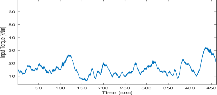
(a) wind speed 5 m/s

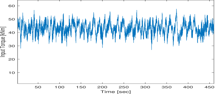
(b) wind speed 13 m/s

Figure 29: FAST simulation of the high speed shaft torque for different turbulent wind condition

A.1 Equation of motion

In order to describe the model with a single equation, we consider the following coordinate

$$\bar{x}(\bar{t})=r_{1}\phi_{1}(\bar{t})-r_{2}\phi_{2}(\bar{t})-\bar{e}(\bar{t}),$$ (29)

where $\phi_{i}(\bar{t})$ stands for the torsional displacement of the $i$-th gear while $r_{i}$ is its radius.

The coordinate $\bar{x}(\bar{t})$ is given by the difference between the dynamic transmission error and the static transmission error. Moreover, through $\bar{x}(\bar{t})$ the model’s equation of motion yields the following formulation (Antoniadou et al.,, 2015; Kahraman and Singh,, 1991)

$$m_{c}\ddot{\bar{x}}(\bar{t})+\bar{C}\dot{\bar{x}}(\bar{t})+\bar{K}(\bar{t})B(\bar{x}(\bar{t}))=\bar{F}_{m}+\bar{F}_{te}(\bar{t})+\bar{F}_{var}(\bar{t}),$$ (30)

where

$$m_{c}=\frac{I_{1}I_{2}}{I_{1}r_{2}^{2}+I_{2}r_{1}^{2}},\quad\bar{F}_{m}=\frac{\bar{T}_{1m}}{r_{1}}=\frac{\bar{T}_{2m}}{r_{2}},$$ (31)

$$\bar{F}_{te}(\bar{t})=-m_{c}\ddot{\bar{e}}(\bar{t})=-\sum_{j=1}^{\infty}F_{tej}(j\bar{\Omega}_{mesh})^{2}\cos(j\bar{\Omega}_{mesh}\bar{t}),$$ (32)

with $I_{i}$ mass moment of inertia of the $i$-th gear and $F_{tej}=\bar{e}_{j}$. Moreover, concerning the quantities that involve the torque obtained via the FAST code:

$$\bar{F}_{var}(\bar{t})=\frac{\bar{T}_{1var}(\bar{t})}{Nr_{1}},$$ (33)

where $N$ is a normalization constant. The normalization constant is included because the FAST simulations correspond to a different physical system. Thus, it is needed to adapt the magnitude of the fluctuations to our setting. $\bar{F}_{m}$ represents the mean force excitations while $\bar{F}_{te}$ and $\bar{F}_{var}$ pertain to internal excitations related to the static transmission error and external excitations related to wind turbulence, respectively. Lastly, the backlash function $B(\bar{x}(\bar{t}))$ is defined as

$$B(\bar{x}(\bar{t}))=\left\{\begin{array}[]{lr}\bar{x}(\bar{t})-b_{g},&\text{for }\bar{x}(\bar{t})\geq b_{g}\\ 0,&\text{for }-b_{g}<\bar{x}(\bar{t})<b_{g}\\ \bar{x}(\bar{t})+b_{g},&\text{for }\bar{x}(\bar{t})\leq-b_{g}\end{array}\right\},$$ (34)

where $2b_{g}$ represents the total gear backlash. The backlash function controls the contact between teeth and incorporates in the model the fact that occasionally contact is lost (Fig. 28).

A.1.1 Dimensionless equation of motion.

The equation of motion (30) can be written in a dimensionless form (Antoniadou et al.,, 2015; Kahraman and Singh,, 1991) by setting : $x(\bar{t})=\frac{\bar{x}(\bar{t})}{b_{g}}$, $w_{n}=\sqrt{\frac{\bar{K}_{m}}{m_{c}}}$, $z=\frac{\bar{C}}{2\sqrt{m_{c}\bar{K}_{m}}}$, $K(\bar{t})=\frac{\bar{K}(\bar{t})}{\bar{K}_{m}}$, $F_{te}(\bar{t})=\frac{\bar{F}_{te}(\bar{t})}{m_{c}b_{g}w_{n}^{2}}=-m_{c}\frac{\ddot{\bar{e}}(\bar{t})}{m_{c}b_{g}w_{n}^{2}}$, $F_{var}(\bar{t})=\frac{\bar{F}_{var}(\bar{t})}{m_{c}b_{g}w_{n}^{2}}$ and $t=w_{n}\bar{t}$. The meshing frequency can be written in a nondimensional form as well, i.e., $\Omega_{mesh}=\frac{\bar{\Omega}_{mesh}}{w_{n}}$. The nondimensional form of the equation of motion (30) is

$$\ddot{x}(t)+2z\dot{x}(t)+K(t)B(x(t))=F_{m}+F_{te}(t)+F_{var}(t)$$ (35)

where the dimensionless backlash function is defined in (17).

Table 3: Simulation parameters

Parameter	Value	Parameter	Value
$I_{1,2}$	$0.00115(\text{Kg}\;\text{m}^{2})$	$F_{m}$	0.1
$m_{c}$	$0.23\text{(Kg)}$	$F_{te1}$	0.01
$r_{1,2}$	0.0 5(m)	$F_{te2}$	0.004
number of teeth	16	$F_{te3}$	0.002
$\bar{K}_{m}$	$3.8\cdot 10^{8}\left(\frac{\text{N}}{\text{m}}\right)$	$K_{1}$	0.2
$b_{g}$	$0.1\cdot 10^{-3}(m)$	$K_{2}$	0.1
$z$	0.05	$K_{3}$	0.05
$\Omega_{mesh}$	0.5	$N$	10

A.2 Parameter settings

The parameters for the experiments reported in this paper are given in Table 3. We also performed additional experiments on signal simulated modifying the parameters related to the internal excitations and changing the severity of the damage. Table 4 shows the three different parameter settings we used in our simulation model to generate acceleration signals affected by different gearbox internal excitations. The parameters have been modified in a combined fashion, and their variation affects the simulated signals locally but not their global structure. For what concerns the severity of the damage, in the simulations analyzed and illustrated in this work, the crack of a gear’s tooth is modelled by decreasing the dimensionless mesh stiffness function by 13 % of its nominal stiffness. Over our experiments, we considered two additional severity conditions. Specifically, we reduced the mesh stiffness function by 10 % and 16 %. Thus we considered two additional scenarios where the severity of the damage either increases or decreases. Overall we considered three conditions for the internal excitation parameters, three damage severities and two wind conditions. The combination of these allowed us to simulate eighteen different scenarios on which to test our method

Table 4: Parameter settings for gearbox internal excitations

Parameter	first setting	second setting	third setting
$F_{te1}$	0.01	0.02	0.003
$F_{te2}$	0.004	0.001	0.002
$F_{te3}$	0.002	0.009	0.004

Appendix B

Table 5: Parameter choices for the different operating conditions of the experimental dataset

Operating conditions (Angular speed $-$ Load)	Delay “ $d$ ” (Snaphots $-$ Time [s])	Length acceleration signal (Snaphots $-$ Time [s])	Decomposition levels
30Hz $-$ High	33333 $-$ 0.5000 s	48333 $-$ 0.7250 s	8
35Hz $-$ High	28572 $-$ 0.4286 s	43572 $-$ 0.6536 s	8
40Hz $-$ Low	24999 $-$ 0.3750 s	39999 $-$ 0.6000 s	8
45Hz $-$ High	22221 $-$ 0.3333 s	37221 $-$ 0.5583 s	8
500Hz $-$ Low	19998 $-$ 0.3000 s	34998 $-$ 0.5250 s	8

References

- Antoni, (2006) Antoni, J. (2006). The spectral kurtosis: a useful tool for characterising non-stationary signals. Mechanical Systems and Signal Processing, 20(2):282–307.
- Antoni and Randall, (2002) Antoni, J. and Randall, R. B. (2002). Differential diagnosis of gear and bearing faults. Journal of Vibration and Acoustics, 124(2):165–171.
- Antoniadou et al., (2015) Antoniadou, I., Manson, G., Staszewski, W., Barszcz, T., and Worden, K. (2015). A time–frequency analysis approach for condition monitoring of a wind turbine gearbox under varying load conditions. Mechanical Systems and Signal Processing, 64-65:188–216.
- Antoniadou et al., (2013) Antoniadou, I., Worden, K., Manson, G., Dervilis, N., Taylor, S., and Farrar, C. R. (2013). Damage detection in RAPTOR telescope systems using time-frequency analysis methods. Key Engineering Materials, 588:43–53.
- Arbabi and Mezić, (2017) Arbabi, H. and Mezić, I. (2017). Ergodic theory, dynamic mode decomposition, and computation of spectral properties of the koopman operator. SIAM Journal on Applied Dynamical Systems, 16(4):2096–2126.
- Avila and Mezić, (2020) Avila, A. M. and Mezić, I. (2020). Data-driven analysis and forecasting of highway traffic dynamics. Nature Communications, 11(1).
- Badaoui et al., (2004) Badaoui, M., Guillet, F., and Danière, J. (2004). New applications of the real cepstrum to gear signals, including definition of a robust fault indicator. Mechanical Systems and Signal Processing, 18(5):1031–1046.
- Bir, (2005) Bir, G. (2005). User’s guide to BModes (software for computing rotating beam-coupled modes). Technical report, Office of Scientific and Technical Information (OSTI).
- Brunton et al., (2017) Brunton, S. L., Brunton, B. W., Proctor, J. L., Kaiser, E., and Kutz, J. N. (2017). Chaos as an intermittently forced linear system. Nature Communications, 8(1).
- Clainche and Vega, (2017) Clainche, S. L. and Vega, J. M. (2017). Higher order dynamic mode decomposition. SIAM Journal on Applied Dynamical Systems, 16(2):882–925.
- Clainche and Vega, (2018) Clainche, S. L. and Vega, J. M. (2018). Analyzing nonlinear dynamics via data-driven dynamic mode decomposition-like methods. Complexity, 2018:1–21.
- Dang et al., (2018) Dang, Z., Lv, Y., Li, Y., and Wei, G. (2018). Improved dynamic mode decomposition and its application to fault diagnosis of rolling bearing. Sensors, 18(6):1972.
- Dao et al., (2019) Dao, C., Kazemtabrizi, B., and Crabtree, C. (2019). Wind turbine reliability data review and impacts on levelised cost of energy. Wind Energy, 22(12):1848–1871.
- del Rincon et al., (2012) del Rincon, A. F., Viadero, F., Iglesias, M., de Juan, A., Garcia, P., and Sancibrian, R. (2012). Effect of cracks and pitting defects on gear meshing. Proceedings of the Institution of Mechanical Engineers, Part C: Journal of Mechanical Engineering Science, 226(11):2805–2815.
- Doebling et al., (1996) Doebling, S., Farrar, C., Prime, M., and Shevitz, D. (1996). Damage identification and health monitoring of structural and mechanical systems from changes in their vibration characteristics: A literature review. Technical report, Office of Scientific and Technical Information (OSTI).
- Du et al., (2006) Du, P., Kibbe, W. A., and Lin, S. M. (2006). Improved peak detection in mass spectrum by incorporating continuous wavelet transform-based pattern matching. Bioinformatics, 22(17):2059–2065.
- Erichson et al., (2016) Erichson, N. B., Brunton, S. L., and Kutz, J. N. (2016). Compressed dynamic mode decomposition for background modeling. Journal of Real-Time Image Processing, 16(5):1479–1492.
- Errichello, (2002) Errichello, R. (2002). How to analyze gear failures. Practical Failure Analysis, 2(6):8–16.
- Feng et al., (2012) Feng, Z., Liang, M., Zhang, Y., and Hou, S. (2012). Fault diagnosis for wind turbine planetary gearboxes via demodulation analysis based on ensemble empirical mode decomposition and energy separation. Renewable Energy, 47:112–126.
- Feng et al., (2019) Feng, Z., Zhu, W., and Zhang, D. (2019). Time-frequency demodulation analysis via vold-kalman filter for wind turbine planetary gearbox fault diagnosis under nonstationary speeds. Mechanical Systems and Signal Processing, 128:93–109.
- Ge et al., (2018) Ge, H., Chen, G., Yu, H., Chen, H., and An, F. (2018). Theoretical analysis of empirical mode decomposition. Symmetry, 10(11):623.
- Harmer et al., (2008) Harmer, K., Howells, G., Sheng, W., Fairhurst, M., and Deravi, F. (2008). A peak-trough detection algorithm based on momentum. In 2008 Congress on Image and Signal Processing. IEEE.
- Héas and Herzet, (2016) Héas, P. and Herzet, C. (2016). Low-rank dynamic mode decomposition: Optimal solution in polynomial-time.
- Hemati et al., (2017) Hemati, M. S., Rowley, C. W., Deem, E. A., and Cattafesta, L. N. (2017). De-biasing the dynamic mode decomposition for applied koopman spectral analysis of noisy datasets. Theoretical and Computational Fluid Dynamics, 31(4):349–368.
- Hu et al., (2019) Hu, A., Xiang, L., Xu, S., and Lin, J. (2019). Frequency loss and recovery in rolling bearing fault detection. Chinese Journal of Mechanical Engineering, 32(1).
- Hu et al., (2018) Hu, Y., Tu, X., Li, F., and Meng, G. (2018). Joint high-order synchrosqueezing transform and multi-taper empirical wavelet transform for fault diagnosis of wind turbine planetary gearbox under nonstationary conditions. Sensors, 18(2):150.
- Huang et al., (1998) Huang, N. E., Shen, Z., Long, S. R., Wu, M. C., Shih, H. H., Zheng, Q., Yen, N.-C., Tung, C. C., and Liu, H. H. (1998). The empirical mode decomposition and the hilbert spectrum for nonlinear and non-stationary time series analysis. Proceedings of the Royal Society of London. Series A: Mathematical, Physical and Engineering Sciences, 454(1971):903–995.
- Inalpolat and Kahraman, (2010) Inalpolat, M. and Kahraman, A. (2010). A dynamic model to predict modulation sidebands of a planetary gear set having manufacturing errors. Journal of Sound and Vibration, 329(4):371–393.
- Ingabire et al., (2021) Ingabire, H. N., Wu, K., Amos, J. T., He, S., Peng, X., Wang, W., Li, M., Chen, J., Feng, Y., Rao, N., and Ren, P. (2021). Analysis of ECG signals by dynamic mode decomposition. IEEE Journal of Biomedical and Health Informatics, pages 1–1.
- Jordanov and Hall, (2002) Jordanov, V. and Hall, D. (2002). Digital peak detector with noise threshold. In 2002 IEEE Nuclear Science Symposium Conference Record. IEEE.
- Junsheng et al., (2007) Junsheng, C., Dejie, Y., and Yu, Y. (2007). The application of energy operator demodulation approach based on EMD in machinery fault diagnosis. Mechanical Systems and Signal Processing, 21(2):668–677.
- Kahraman and Singh, (1991) Kahraman, A. and Singh, R. (1991). Interactions between time-varying mesh stiffness and clearance non-linearities in a geared system. Journal of Sound and Vibration, 146(1):135–156.
- Korda and Mezić, (2017) Korda, M. and Mezić, I. (2017). On convergence of extended dynamic mode decomposition to the koopman operator. Journal of Nonlinear Science, 28(2):687–710.
- Kumar et al., (2021) Kumar, R., Ismail, M., Zhao, W., Noori, M., Yadav, A. R., Chen, S., Singh, V., Altabey, W. A., Silik, A. I. H., Kumar, G., Kumar, J., and Balodi, A. (2021). Damage detection of wind turbine system based on signal processing approach: a critical review. Clean Technologies and Environmental Policy, 23(2):561–580.
- (35) Kutz, J. N., Brunton, S. L., Brunton, B. W., and Proctor, J. L. (2016a). Dynamic Mode Decomposition. Society for Industrial and Applied Mathematics.
- (36) Kutz, J. N., Fu, X., and Brunton, S. L. (2016b). Multiresolution dynamic mode decomposition. SIAM Journal on Applied Dynamical Systems, 15(2):713–735.
- Li et al., (2019) Li, X., Chen, K., Huangfu, Y., Ma, H., Zhao, B., and Yu, K. (2019). Vibration characteristic analysis of spur gear systems under tooth crack or fracture. Journal of Low Frequency Noise, Vibration and Active Control, 40(1):135–153.
- Ma et al., (2014) Ma, H., Song, R., Pang, X., and Wen, B. (2014). Fault feature analysis of a cracked gear coupled rotor system. Mathematical Problems in Engineering, 2014:1–22.
- Mann and Kutz, (2016) Mann, J. and Kutz, J. N. (2016). Dynamic mode decomposition for financial trading strategies. Quantitative Finance, 16(11):1643–1655.
- Matsumoto and Indinger, (2017) Matsumoto, D. and Indinger, T. (2017). On-the-fly algorithm for dynamic mode decomposition using incremental singular value decomposition and total least squares.
- Mba et al., (2017) Mba, C. U., Marchesiello, S., Fasana, A., and Garibaldi, L. (2017). Gearbox damage identification and quantification using stochastic resonance. Mechanics & Industry, 18(7):705.
- McFadden, (1987) McFadden, P. (1987). A revised model for the extraction of periodic waveforms by time domain averaging. Mechanical Systems and Signal Processing, 1(1):83–95.
- McFadden, (1986) McFadden, P. D. (1986). Detecting fatigue cracks in gears by amplitude and phase demodulation of the meshing vibration. Journal of Vibration and Acoustics, 108(2):165–170.
- Mohamed et al., (2018) Mohamed, A. S., Sassi, S., and Paurobally, M. R. (2018). Model-based analysis of spur gears’ dynamic behavior in the presence of multiple cracks. Shock and Vibration, 2018:1–20.
- Peng and Chu, (2004) Peng, Z. and Chu, F. (2004). Application of the wavelet transform in machine condition monitoring and fault diagnostics: a review with bibliography. Mechanical Systems and Signal Processing, 18(2):199–221.
- PHMSociety, (2009) PHMSociety (2009). PHM Challenge Competition Datase. https://phmsociety.org/public-data-sets/.
- Proctor and Eckhoff, (2015) Proctor, J. L. and Eckhoff, P. A. (2015). Discovering dynamic patterns from infectious disease data using dynamic mode decomposition. International Health, 7(2):139–145.
- Randall, (2021) Randall, R. B. (2021). Vibration-based Condition Monitoring. John Wiley and Sons.
- Rao et al., (2011) Rao, K. R., Kim, D. N., and Hwang, J. J. (2011). Fast Fourier Transform - Algorithms and Applications. Springer-Verlag GmbH.
- Redl et al., (2021) Redl, C., Hein, F., Buck, M., Graichen, P., and Jones, D. (2021). The european power sector in 2020. up-to-date analysis on the electricity transition. Technical report, Agora Energiewende.
- Salameh et al., (2018) Salameh, J. P., Cauet, S., Etien, E., Sakout, A., and Rambault, L. (2018). Gearbox condition monitoring in wind turbines: A review. Mechanical Systems and Signal Processing, 111:251–264.
- Schmid, (2010) Schmid, P. J. (2010). Dynamic mode decomposition of numerical and experimental data. Journal of Fluid Mechanics, 656:5–28.
- Sharma, (2021) Sharma, V. (2021). A review on vibration-based fault diagnosis techniques for wind turbine gearboxes operating under nonstationary conditions. Journal of The Institution of Engineers (India): Series C, 102(2):507–523.
- Sharma and Parey, (2016) Sharma, V. and Parey, A. (2016). Gearbox fault diagnosis using RMS based probability density function and entropy measures for fluctuating speed conditions. Structural Health Monitoring, 16(6):682–695.
- Stander and Heyns, (2005) Stander, C. and Heyns, P. (2005). Instantaneous angular speed monitoring of gearboxes under non-cyclic stationary load conditions. Mechanical Systems and Signal Processing, 19(4):817–835.
- Staszewski and Tomlinson, (1994) Staszewski, W. and Tomlinson, G. (1994). Application of the wavelet transform to fault detection in a spur gear. Mechanical Systems and Signal Processing, 8(3):289–307.
- Staszewski et al., (1997) Staszewski, W., Worden, K., and Tomlinson, G. (1997). Time–frequency analysis in gearbox fault detection using the Wigner–Ville distribution and pattern recognition. Mechanical Systems and Signal Processing, 11(5):673–692.
- Tirunagari et al., (2017) Tirunagari, S., Kouchaki, S., Poh, N., Bober, M., and Windridge, D. (2017). Dynamic Mode Decomposition for Univariate Time Series: Analysing Trends and Forecasting. working paper or preprint.
- Tu et al., (2014) Tu, J. H., Rowley, C. W., Luchtenburg, D. M., Brunton, S. L., and Kutz, J. N. (2014). On dynamic mode decomposition: Theory and applications. J Comput Dyn, 1:391–421.
- Wu and Huang, (2009) Wu, Z. and Huang, N. E. (2009). Ensemble Empirical Mode Decomposition: A noise-assisted data analysis method. Advances in Adaptive Data Analysis, 01(01):1–41.
- Xin et al., (2020) Xin, G., Hamzaoui, N., and Antoni, J. (2020). Extraction of second-order cyclostationary sources by matching instantaneous power spectrum with stochastic model – application to wind turbine gearbox. Renewable Energy, 147:1739–1758.
- Xu et al., (2016) Xu, G., Yang, Z., and Wang, S. (2016). Study on mode mixing problem of empirical mode decomposition. In Proceedings of the 2016 Joint International Information Technology, Mechanical and Electronic Engineering. Atlantis Press.