Transverse spherocity dependence of azimuthal anisotropy in heavy-ion collisions
at the LHC using a multi-phase transport model

Abstract

One of the event shape observables, the transverse spherocity ($S_{0}$), has been studied successfully in small collision systems such as proton-proton collisions at the LHC as a tool to separate jetty and isotropic events. It has a unique capability to distinguish events based on their geometrical shapes. In our work, we report the first implementation of transverse spherocity in heavy-ion collisions using a multi-phase transport model (AMPT). We have performed an extensive study of azimuthal anisotropy of charged particles produced in heavy-ion collisions as a function of transverse spherocity ($S_{0}$). We have followed the two-particle correlation (2PC) method to estimate the elliptic flow ($v_{2}$) in different centrality classes in Pb-Pb collisions at $\sqrt{s_{\rm NN}}=5.02$ TeV for high-$S_{0}$, $S_{0}$-integrated and low-$S_{0}$ events. We found that transverse spherocity successfully differentiates heavy-ion collisions’ event topology based on their geometrical shapes, i.e., high and low values of spherocity. The high-$S_{0}$ events have nearly zero elliptic flow, while the low-$S_{0}$ events contribute significantly to the elliptic flow of spherocity-integrated events.

1 Introduction

The production of a hot and dense, deconfined state of matter known as the quark-gluon plasma (QGP) has already been established in heavy-ion collisions at the Large Hadron Collider (LHC) at CERN, Switzerland, and Relativistic Heavy Ion Collider (RHIC) at BNL, USA. Recent studies at the LHC show heavy-ion-like features such as ridge-like structures [1] and strangeness enhancements [2] in pp collisions. To understand the system dynamics and production of jets in pp collisions, an event shape observable, known as the transverse spherocity ($S_{0}$), has been introduced recently at the LHC [3, 4, 5, 6, 7]. These studies show that transverse spherocity ($S_{0}$) has unique capabilities to distinguish events based on its geometrical shapes i.e. jetty and isotropic events. The study of transverse spherocity in heavy-ion collisions may reveal new and unique physics results where the formation of QGP is already known. This study in heavy-ion collisions shall also complement the current event shape approach based on flow vector analysis at the LHC [8, 9].

In this work [10], we report the first implementation of transverse spherocity in heavy-ion collisions using a multi-phase transport (AMPT) model [11]. We have performed an extensive study of azimuthal anisotropy of charged particles produced in Pb-Pb collisions at $\sqrt{s_{\rm NN}}=5.02$ TeV as a function of transverse spherocity ($S_{0}$). We have followed the two-particle correlation (2PC) method to estimate the elliptic flow ($v_{2}$) and subtract non-flow from our calculations by following standard experimental procedures.

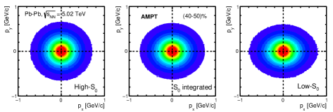
Figure 1: (Color Online) Transverse momentum space correlation ($p_{\rm y}$ vs. $p_{\rm x}$) for different spherocity classes in (40-50)% central Pb-Pb collisions at $\sqrt{s_{\rm NN}}=5.02$ TeV using AMPT model. (Fig. 2 [10])

Transverse spherocity ($S_{0}$) is an event property which is also a collinear and infrared safe quantity [3, 4, 5] and defined as follows,

$$S_{0}=\frac{\pi^{2}}{4}\bigg{(}\frac{\Sigma_{i}~{}|\vec{p}_{T_{i}}\times\hat{n}|}{\Sigma_{i}~{}p_{T_{i}}}\bigg{)}^{2}.$$ (1)

Here, $\hat{n}(n_{T},0)$ is a unit vector known as the spherocity axis, which minimizes the ratio in Eq. 1. For jetty events $S_{0}\approx 0$ and for isotropic events $S_{0}\approx 1$ [7]. We have used the mid-rapidity ($|\eta|<0.8$) spherocity distribution with $p_{\rm T}>0.15$ GeV/c with events having at least five such tracks to meet similar conditions as in the ALICE experiment at the LHC. The low-$S_{0}$ and high-$S_{0}$ events represent the events lying in the bottom 20% and top 20% in the $S_{0}$ distributions whereas $S_{0}$-integrated events take all events into account.

Figure 1 represents the transverse momentum space correlation ($p_{\rm y}$ vs. $p_{\rm x}$) for high-$S_{0}$, $S_{0}$-integrated and low-$S_{0}$ events in (40-50)% central Pb-Pb collisions at $\sqrt{s_{\rm NN}}=5.02$ TeV using AMPT model. The elliptic flow in $S_{0}$-integrated events can be clearly seen from the elliptic shape of the correlation plot. This is indeed credited to the initial pressure gradient caused due to the initial almond-shaped nuclear overlap region in semi-central collisions, which is then translated to the momentum space ($p_{\rm x}>p_{\rm y}$) correlations. The interesting thing is that the high-$S_{0}$ events show almost spherical momentum correlation indicating the presence of nearly zero elliptic flow in such events. Whereas the events with low-$S_{0}$ show a greater elliptical shape correlation. That indicates low-$S_{0}$ events should be more elliptic and therefore contribute more towards $v_{2}$.

2 Results and Discussions

To estimate the elliptic flow we have used the two-particle correlation method (2PC) [8, 12]. The two particle correlation function $C(\Delta\eta,\Delta\phi)$ is constructed by taking the ratios of same-event pairs $S(\Delta\eta,\Delta\phi)$ to mixed-event pairs $B(\Delta\eta,\Delta\phi)$ given by,

$$C(\Delta\eta,\Delta\phi)=\frac{S(\Delta\eta,\Delta\phi)}{B(\Delta\eta,\Delta\phi)}.$$ (2)

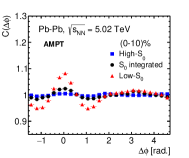
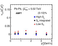
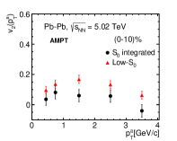
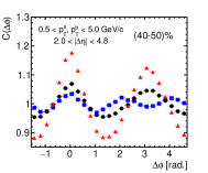
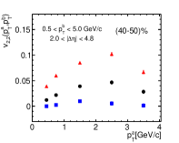
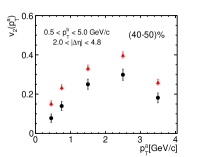
Figure 2: (Color Online) First column: One dimensional azimuthal correlation of charged particles, second column: two particle elliptic flow coefficient ($v_{2,2}(p_{T}^{a},p_{T}^{b})$) of charged particles as a function of $p_{T}^{a}$, and third column: single particle elliptic flow coefficient ($v_{2}(p_{T}^{a})$) of charged particles as a function of $p_{T}^{a}$ for low-$S_{0}$, high-$S_{0}$ and $S_{0}$-integrated events in Pb–Pb collisions at $\sqrt{s_{\rm NN}}=5.02$ TeV for 0%–10% (top), 40%–50% (bottom) centrality classes using AMPT model. (Figs. 4-6 [10])

The one dimensional correlation function ($C(\Delta\phi)$) is then calculated by integrating all the pairs with pseudorapidity gap $2.0<|\Delta\eta|<4.8$. This step helps in reducing the contributions from non-flow effects [8]. From the $C(\Delta\phi)$ distribution, the two particle flow coefficient ($v_{2,2}(p_{\rm T}^{a},p_{\rm T}^{b})$) could be easily obtained as [13, 14, 15],

$$v_{n,n}(p_{\rm T}^{a},p_{\rm T}^{b})=\langle cos(n\Delta\phi)\rangle=\frac{\sum_{m=1}^{N}cos(n\Delta\phi_{m})\times C(\Delta\phi_{m})}{\sum_{m=1}^{N}C(\Delta\phi_{m})}.$$ (3)

where, $N$ = 200 is the number of $\Delta\phi$ bins in the range $-\pi/2<\Delta\phi<3\pi/2$. Here, $v_{n,n}$ are symmetric functions with respect to $p_{\rm T}^{a}$ and $p_{\rm T}^{b}$. The single particle flow coefficient could be obtained as,

$$v_{n,n}(p_{\rm T}^{a},p_{\rm T}^{b})=v_{n}(p_{\rm T}^{a})v_{n}(p_{\rm T}^{b}).$$ (4)

Figure 2 first column shows that the shape and nature of the 1D azimuthal correlation vary with spherocity, and one can observe that the amplitude of the correlation is greater in low-$S_{0}$, intermediate in $S_{0}$-integrated and lower in high-$S_{0}$ events. Again, the amplitude of the correlation is more in semi-central collisions compared to most central collisions. Figure 2 second column represents the two particle elliptic flow co-efficient $v_{2,2}(p_{T}^{a},p_{T}^{b})$ as a function of spherocity. Here, $v_{2,2}(p_{T}^{a},p_{T}^{b})$ has strong centrality dependence with showing greater values towards semi-central collisions. As far as spherocity is concerned, the high-$S_{0}$ events are found to have nearly zero elliptic flow while the low-$S_{0}$ events contribute significantly to elliptic flow of spherocity-integrated events. This is evident from the third column of Fig. 2.

3 Summary

In summary, we found that transverse spherocity successfully differentiates heavy-ion collisions’ event topology based on their geometrical shapes, i.e. high and low values of spherocity ($S_{0}$). The high-$S_{0}$ events are found to have nearly zero elliptic flow, while the low-$S_{0}$ events contribute significantly to the elliptic flow of spherocity-integrated events. Transverse spherocity is anti-correlated to elliptic flow.

References

- [1] V. Khachatryan et al. [CMS], Phys. Lett. B 765 (2017), 193
- [2] J. Adam et al. [ALICE], Nature Phys. 13 (2017), 535
- [3] E. Cuautle, R. Jimenez, I. Maldonado, A. Ortiz, G. Paic and E. Perez, [arXiv:1404.2372 [hep-ph]].
- [4] A. Ortiz, G. Paić and E. Cuautle, Nucl. Phys. A 941 (2015), 78
- [5] G. P. Salam, Eur. Phys. J. C 67 (2010), 637
- [6] G. Bencédi [ALICE], Nucl. Phys. A 982 (2019), 507
- [7] S. Acharya et al. [ALICE], Eur. Phys. J. C 79 (2019), 857
- [8] G. Aad et al. [ATLAS], Phys. Rev. C 92 (2015), 034903
- [9] M. Masera, G. Ortona, M. G. Poghosyan and F. Prino, Phys. Rev. C 79 (2009), 064909
- [10] N. Mallick, R. Sahoo, S. Tripathy and A. Ortiz, J. Phys. G 48 (2021), 045104
- [11] Z. W. Lin, C. M. Ko, B. A. Li, B. Zhang and S. Pal, Phys. Rev. C 72 (2005), 064901
- [12] S. A. Voloshin, A. M. Poskanzer and R. Snellings, Landolt-Bornstein 23 (2010), 293
- [13] G. Aad et al. [ATLAS], Phys. Rev. C 86 (2012), 014907
- [14] S. Chatrchyan et al. [CMS], Phys. Rev. C 89 (2014), 044906
- [15] K. Aamodt et al. [ALICE], Phys. Lett. B 708 (2012), 249