Eigenstate thermalization hypothesis and its deviations from random-matrix theory beyond the thermalization time

Abstract

The Eigenstate Thermalization Hypothesis (ETH) explains emergence of the thermodynamic equilibrium in isolated quantum many-body systems by assuming a particular structure of observable’s matrix elements in the energy eigenbasis. Schematically, it postulates that off-diagonal matrix elements are random numbers and the observables can be described by Random Matrix Theory (RMT). To what extent a RMT description applies, more precisely at which energy scale matrix elements of physical operators become truly uncorrelated, is however not fully understood. We study this issue by introducing a novel numerical approach to probe correlations between matrix elements for Hilbert-space dimensions beyond those accessible by exact diagonalization. Our analysis is based on the evaluation of higher moments of operator submatrices, defined within energy windows of varying width. Considering nonintegrable quantum spin chains, we observe that matrix elements remain correlated even for narrow energy windows corresponding to time scales of the order of thermalization time of the respective observables. We also demonstrate that such residual correlations between matrix elements are reflected in the dynamics of out-of-time-ordered correlation functions.

Introduction. In the overwhelming majority of cases, isolated quantum many-body systems undergoing unitary time evolution are expected to reach thermal equilibrium at long times dalessio2016 ; polkovnikov2011 ; gogolin2016 ; borgonovi2016 ; Mori2018 . During the thermalization process, local memory of the initial nonequilibrium state is lost and observables reach a constant value that agrees with an appropriate thermodynamic ensemble average, as observed in some recent experiments, see, e.g., Trotzky2012 ; Kaufmann2016 ; Lukin19 ; Tang18 ; Clos16 ; Kim18 ; Lepoutre19 ; Hofferberth07 .

Motivated by seminal works on quantum chaos and random-matrix theory (RMT), see book-casati ; qc-Brody ; book-Haake ; qc-Izrailev ; qc-Zelevinsky ; Guhr1998 for reviews, including intimate connections to transport in mesoscopic systems Alhassid2000 ; Beenakker1997 , the eigenstate thermalization hypothesis (ETH) explains eventual thermalization by postulating a particular structure of matrix elements of observable ${\cal O}$ in the eigenbasis of a generic Hamiltonian ${\cal H}$ Deutsch91 ; Srednicki94 ; rigol2008 ,

$${\cal O}_{mn}=O(\bar{E})\delta_{mn}+\Omega^{-1/2}(\bar{E})f(\bar{E},\omega)r_{mn}\ ,$$ (1)

where $\omega=E_{m}-E_{n}$, $\bar{E}=(E_{m}+E_{n})/2$, and ${\cal O}_{mn}=\bra{m}{\cal O}\ket{n}$, with $E_{m}$ and $\ket{m}$ denoting the eigenvalues and eigenstates of ${\cal H}$. Moreover, $\Omega(\bar{E})$ is the density of states, $O(\bar{E})$ and $f(\bar{E},\omega)$ are smooth functions, and the $r_{mn}=r_{nm}^{\ast}$ are usually assumed to be independent random Gaussian variables with zero mean and unit variance, see also Jensen1985 ; Feingold1986 ; Feingold1991 for early works on precursors of Eq. (1). While the general features of the ETH have been numerically confirmed for various nonintegrable models steinigeweg2013 ; beugeling2014 ; kim2014 ; Torres-Herrera2014 ; Mondaini2016 ; Mondaini2017 ; jansen2019 ; LeBlond2019 ; Brenes2020 ; Richter2020 ; Noh21 , recent works have proposed further generalizations Richter2019 ; Dymarsky2019 ; Kaneko2020 ; Mierzejewski2020 , and scrutinized detailed aspects such as entanglement structure of highly excited eigenstates Brenes2020_2 , or the presence of rare ETH-violating states Serbyn2020 .

The formulation of the ETH in Eq. (1) may essentially be regarded as an extension of the RMT applied to observables. It builds on earlier sophisticated models to describe physical systems by random matrices such as band matrices Casati1990 ; Fyodorov1991 and embedded ensembles qc-Brody ; Kota2001 ; French1970 ; Flores2001 , which take into account the locality of real systems. Numerical analyses have yielded a convincing agreement with the predictions of Eq. (1), for instance regarding the Gaussianity of the $r_{mn}$ LeBlond2019 ; Luitz2020 , the distribution of transition strengths $|{\cal O}_{mn}|^{2}$ qc-Alhassid ; Alhassid89 ; Barbosa2000 , and the ratio of variances of diagonal and off-diagonal matrix elements dalessio2016 ; Dymarsky:2017zoc ; Mondaini2017 ; jansen2019 . Moreover, statistical properties of matrix elements have been analyzed semiclassically in few-body systems with classically chaotic counterpart Srednicki98 ; Srednicki00 ; Eckhardt95 .

Physical Hamiltonians and observables clearly differ from genuinely random operators qc-Brody (for instance, matrix elements $\bra{m}\sigma_{z}\ket{n}$ of a Pauli operator must be correlated to yield the eigenvalues $\pm 1$). In this context, the question whether and to what extent the $r_{mn}$ in Eq. (1) can indeed be considered as uncorrelated random numbers has attracted increased attention recently Richter2020 ; Dymarsky2018 ; Brenes2021 . In particular, it has been argued that correlations between matrix elements are necessary to explain the growth of out-of-time ordered correlation function (OTOC) Foini2019 ; Chan2019 ; Murthy2019 , which is a central quantity to characterize scrambling in quantum systems Swingle2016 . Using full eigenvalue spectrum of operator submatrices as a sensitive indicator, correlations between matrix elements have been shown to persist to small energy scales, but appear to vanish at even lower $\omega$ Richter2020 . The lack of correlations between $r_{mn}$ at low $\omega$ is consistent with expected universality of the observable’s dynamics at late times Cotler2017 ; Cotler2019 ; Moudgalya2019 ; Schiulaz2019 .

An important and less clear aspect is to connect the onset of RMT behavior, particularly the statistical independence of matrix elements, with the time scale of thermalization. Given a (one-dimensional) quantum many-body system of size $L$, the thermalization time $\tau_{\text{th}}$ of an observable $\mathcal{O}$ is expected to scale as $\tau_{\text{th}}\propto L^{\nu}$, where $\nu\geq 0$ depends on $\mathcal{O}$ and details of the system, e.g., presence of conservation laws Bertini2021 , or disorder Abanin2019 . Somewhat unexpectedly, it was analytically shown in Dymarsky2018 that in one dimensional systems, macroscopic thermalization dynamics prevents matrix elements of $\mathcal{O}$ from becoming truly uncorrelated above a smaller energy scale $\Delta E_{\text{RMT}}\propto 1/(\tau_{\text{th}}L)$, and the system’s dynamics is fully described by RMT only at much later times, $T_{\text{RMT}}\propto 1/\Delta E_{\text{RMT}}\propto\tau_{\text{th}}L$. This has consequences for instance for the dynamics of certain initial states with a macroscopic spatial inhomogeneity of a conserved quantity, e.g., energy, which will display nontrivial dynamics even for $t>\tau_{\text{th}}$ and saturate into exponentially small fluctuations $\propto e^{-L}$ only at parametrically longer $t$ Dymarsky2018 .

We note that the time $T_{\text{RMT}}$ explored here and in Dymarsky2018 , which marks the absence of correlations between matrix elements, is different from the so-called “Thouless time” Thouless1974 , see thouless-time for details, which has also been associated to the applicability of RMT to the energy spectrum, signaled by a ramp in the spectral form factor Schiulaz2019 ; Prosen2020 ; Kos2021 ; Moudgalya2021 ; Piotr20 .

From a numerical point of view, a major complication to study matrix elements is given by the restriction of full exact diagonalization (ED) to small system sizes, such that the analysis of low-frequency or, correspondingly, long-time regimes is plagued by severe finite-size effects. In this Letter, we introduce a novel numerical approach based on quantum typicality (see Jin2021 ; Heitmann2020 and references therein). We show that moments of operator submatrices, defined within energy windows of varying width, can be evaluated for system sizes beyond the range of ED, and provide a sensitive probe to study the presence of correlations between matrix elements. This allows us to shed new light on residual deviations of physical operators from genuine RMT ensembles, including the Gaussian Orthogonal Ensemble (GOE), which is expected to emerge for the models and operators with real and symmetric matrix representation considered here. For nonintegrable quantum spin chains, our analysis shows that matrix elements remain correlated even in narrow energy windows corresponding to time scales around the thermalization time of the respective observable. For shorter times, the residual correlations between matrix elements are manifest in the nontrivial dynamics of suitably defined OTOCs within such energy windows.

Setup. We consider submatrices ${\cal O}^{T}$ defined within energy windows of width $2\pi/T$ Dymarsky:2017zoc ; Dymarsky2018 ; Richter2020 ,

$${\cal O}_{mn}^{T}=\langle m|P_{T}{\cal O}P_{T}|n\rangle=\begin{cases}{\cal O}_{mn}\ ,&|E_{m,n}-E_{0}|\leq\frac{\pi}{T}\\ 0\ ,&\text{otherwise}\end{cases}\ ,$$ (2)

where $P_{T}=\sum_{|E_{m}-E_{0}|\leq\frac{\pi}{T}}|m\rangle\langle m|$ is a projection on eigenstates of ${\cal H}$ centered around $E_{0}$. Parameter $T$ controlling the size of the submatrix determines characteristic time scale (matrix elements at low $\omega$ contribute to dynamics at long times). We will compare the energy scale $1/T$, where the ${\cal O}_{mn}^{T}$ become uncorrelated, with the scale $1/\tau_{\text{th}}$ set by thermalization time of ${\cal O}$. Examples of ${\cal H}$, ${\cal O}$, and a definition of $\tau_{\text{th}}$ are given below.

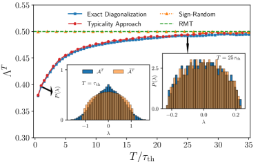
Figure 1: $\Lambda^{T}$ versus $T/\tau_{\text{th}}$ for ${\cal A}$ with $q=L/2$ and $L=16$. Results obtained by the typicality approach, averaged over $500$ states, agree convincingly with ED data. As a comparison, $\Lambda^{T}$ obtained from a sign-randomized operator [Eq. (7)] yields the GOE value $\Lambda^{T}=1/2$. Insets show eigenvalue distributions $P(\lambda)$ of ${\cal A}^{T}$ and $\widetilde{{\cal A}}^{T}$ for different energy windows.

We study the presence of correlations between matrix elements by introducing the ratio $\Lambda^{T}$ of moments of ${\cal O}_{c}^{T}$,

$${\Lambda^{T}={\cal M}_{2}^{2}/{\cal M}_{4}}\ ,\quad{{\cal M}_{k}=\text{Tr}[({\cal O}_{c}^{T})^{k}]/d}\ ,$$ (3)

where $d=\text{Tr}[P_{T}]=\sum_{|E_{m}-E_{0}|\leq\frac{\pi}{T}}1$ and ${\cal O}_{c}^{T}={\cal O}^{T}-\text{Tr}({\cal O}^{T})/d$. If ${\cal O}^{T}$ were to be described by an ideal GOE, its eigenvalues would follow famous Wigner semicircle distribution, implying $\Lambda^{T}_{\text{GOE}}=1/2$. Crucially, as we show in SuppMat , $\Lambda^{T}\simeq 1/2$ can be derived also for weaker conditions on ${\cal O}^{T}$ as long as the ${\cal O}_{mn}^{T}$ are statistically independent. In particular, as discussed in SuppMat and demonstrated below, $\Lambda^{T}\to 1/2$ can serve as a sensitive indicator to locate the energy scale where ${\cal O}_{mn}^{T}$ become uncorrelated and deviations from a strict GOE disappear.

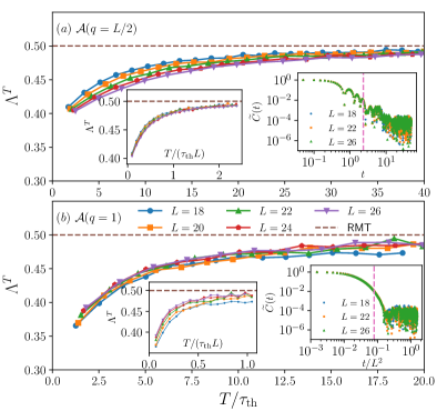
Figure 2: $\Lambda^{T}$ versus $T/\tau_{\text{th}}$ for the density-wave operator ${\cal A}$ with (a) $q=L/2$ and (b) $q=1$. Data are obtained using typicality approach up to $L=26$, averaged over $500\cdot 2^{16-L}$ random states NoteAverage . The dashed line indicates the GOE value $\Lambda^{T}_{\text{GOE}}=0.5$. Insets show $\Lambda^{T}$ versus $T/(\tau_{\text{th}}L)$ and the rescaled correlation function $\widetilde{C}(t)$. The dashed vertical line signals $\tau_{\text{th}}$ according to our definition in the text. The data collapse of $\widetilde{C}(t)$ and $\widetilde{C}(t/L^{2})$ indicates $L$-independence of $\tau_{\text{th}}$ for $q=L/2$ and diffusive behavior $\tau_{\text{th}}\propto L^{2}$ for $q=1$.

Numerical approach. To construct ${\cal O}^{T}$ explicitly without using ED, it is crucial to rewrite $P_{T}$ as $P_{T}=\frac{1}{T}\int_{-\infty}^{+\infty}\text{sinc}(t/T)\exp[-i({\cal H}-E_{0})t]dt$  Dymarsky2018 , where $\text{sinc}(t)=\sin(\pi t)/\pi t$. In particular, by expanding the time evolution operator in terms of Chebyshev polynomials Tal-Ezer1984 ; Dobrovitski2003 ; Weisse2006 and evaluating the integral analytically, one finds SuppMat , $P_{T}=\sum_{k=0}^{\infty}C_{k}T_{k}(\frac{{\cal H}-b}{a})$, where $T_{k}(x)$ are Chebyshev polynomials of the first kind, $C_{k}$ are suitable coefficients SuppMat , and $a=(E_{\text{max}}-E_{\text{min}})/2,\ b=(E_{\text{max}}+E_{\text{min}})/2$, where $E_{\text{max}}$ ($E_{\text{min}}$) is the largest (smallest) eigenvalue of $\cal H$. Exploiting quantum typicality Jin2021 ; Heitmann2020 (see also SuppMat ) one can then calculate the second and the fourth central moments of ${\cal O}^{T}$ as

$${\cal M}_{2}\approx\frac{\langle\psi_{POP}|\psi_{POP}\rangle}{\langle\psi_{P}|\psi_{P}\rangle}\ ,\ {\cal M}_{4}\approx\frac{\langle\psi_{(POP)^{2}}|\psi_{(POP)^{2}}\rangle}{\langle\psi_{P}|\psi_{P}\rangle}\ ,$$ (4)

where $|\psi_{P}\rangle=P_{T}|\psi\rangle$, $|\psi_{POP}\rangle=P_{T}{\cal O}^{T}_{c}P_{T}|\psi\rangle$, $|\psi_{(POP)^{2}}\rangle=(P_{T}{\cal O}^{T}_{c}P_{T})^{2}|\psi\rangle$, and ${\cal O}^{T}_{c}={\cal O}^{T}-\langle\psi_{P}|{\cal O}^{T}|\psi_{P}\rangle/\langle\psi_{P}|\psi_{P}\rangle$. Here, $|\psi\rangle$ is a pure state drawn at random from the unitarily invariant Haar measure Bartsch2009 , i.e., in practice $\ket{\psi}$ is constructed in the computational basis with Gaussian distributed coefficients. The approximation of ${\cal M}_{k}$ in Eq. (4) becomes very accurate for energy windows with sufficiently many eigenstates. For smaller windows with fewer eigenstates, the accuracy can be improved by averaging over multiple realizations of $\ket{\psi}$. The most demanding step of our approach is to restrict the random state to a narrow energy window, $P_{T}|\psi\rangle=\sum_{k=0}^{M}C_{k}T_{k}(\frac{{\cal H}-b}{a})|\psi\rangle$, where $P_{T}$ is approximated by a sum up to $k=M$, which has to be chosen large enough to yield accurate results NoteParameters . Combined with efficient sparse-matrix techniques, ${\cal M}_{k}$ and $\Lambda^{T}$ can then be obtained for Hilbert-space dimensions far beyond the range of the ED. Note that other approaches exist to construct states in a specified energy window Yamaji2018 ; Piotr202 ; Garnerone2013 ; Steinigeweg2014 .

Numerical analysis. We consider one-dimensional mixed-field Ising model, ${\cal H}=\sum_{\ell=1}^{L}{\cal H}^{\ell}$,

$${\cal H}^{\ell}=J\sigma_{z}^{\ell}\sigma_{z}^{\ell+1}+\frac{h_{x}}{2}(\sigma_{x}^{\ell}+\sigma_{x}^{\ell+1})+\frac{h_{z}}{2}(\sigma_{z}^{\ell}+\sigma_{z}^{\ell+1})\ ,$$ (5)

where $\sigma^{\ell}_{x,z}$ are Pauli operators at lattice site $\ell$, $L$ is the length of the chain with periodic boundaries, and $J=h_{x}=1.0$ and $h_{z}=0.5$ in the following. Moreover, we add two defect terms $h_{2}\sigma_{z}^{2}$ and $h_{5}\sigma_{z}^{5}$ with $h_{2}=0.1665$ and $h_{5}=-0.2415$ to lift translational and reflection symmetries, such that our simulations are performed in the full Hilbert space of dimension $2^{L}$. We note that ${\cal H}$ is nonintegrable, fulfills the ETH for these parameters SuppMat , and exhibits diffusive energy transport Kim2013 . We consider energy windows around $E_{0}=0$, corresponding to infinite temperature. We study $\Lambda^{T}$ for two kinds of operators,

$${\cal A}=\frac{1}{\sqrt{L}}\sum_{\ell=1}^{L}\cos\left(\frac{2\pi}{L}q\ell\right){\cal H}^{\ell},\quad{\cal B}=\frac{1}{\sqrt{L}}\sum_{\ell=1}^{L}\sigma_{x}^{\ell}\ ,$$ (6)

where ${\cal B}$ exhibits no transport behavior and decays quickly. In contrast, dynamics of the density-wave operator ${\cal A}$ depends on $q$, with a quick $L$-independent decay for $q=L/2$ and a slow hydrodynamic (diffusive) relaxation in the limit of small $q$ Bertini2021 . For our numerical analysis, operators with short, $L$-independent, $\tau_{\text{th}}$ are beneficial as this allows us to reach regimes $T/\tau_{\text{th}}\gg 1$, which in contrast becomes very costly if $\tau_{\text{th}}\propto L^{2}$ scales diffusively.

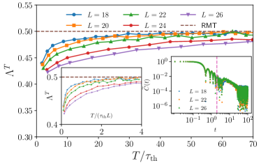
Figure 3: Analogous data as in Fig. 2, but now for ${\cal B}$.

A first glance of how $\Lambda^{T}$ behaves upon varying the width of the energy window is given in Fig. 1, where we consider ${\cal A}$ for a small system with $L=16$ amenable to ED. ED values of $\Lambda^{T}$ show convincing agreement with those obtained using typicality approach for a wide range of $T$. Analyzing $\Lambda^{T}$ behavior, we see that it deviates from the GOE value for small $T$ (i.e., large energy windows), but approaches it for larger $T$. As shown in the insets of Fig. 1, the full eigenvalue distribution $P(\lambda)$ of ${\cal A}^{T}$ is approximately Gaussian for small $T$ ($\Lambda^{T}=1/3$ for strictly Gaussian distributions), while it takes an approximately semicircle shape for larger $T$, indicating a transition to GOE behavior Richter2020 . Importantly, while $\Lambda^{T}$ displays that strict GOE behavior only occurs at large $T$, other common random-matrix indicators, such as the mean ratio of adjacent level spacings $\langle r\rangle$ Oganesyan2007 , turn out to be insensitive to the residual correlations between the ${\cal O}_{mn}^{T}$ at small $T$, see SuppMat . In this context, it is also helpful to evaluate $\Lambda^{T}$ for a sign-randomized version of ${\cal O}^{T}$ Richter2020 ; Cohen2001 ; Kottos2001 ,

$$\widetilde{{\cal O}}_{mn}^{T}=\begin{cases}{\cal O}_{mn}^{T}\ ,&\text{50\% probability}\\ (-1){\cal O}_{mn}^{T}\ ,&\text{50\% probability}\end{cases}\ ,$$ (7)

where potential correlations between the ${\cal O}_{mn}^{T}$ are thus manually destroyed. As shown in Fig. 1, $\widetilde{{\cal A}}^{T}$ indeed yields $\Lambda^{T}\approx 0.5$ with semicircular $P(\lambda)$ for all $T$, which further confirms that $\Lambda^{T}\to 0.5$ is a good indicator for the absence of correlations between matrix elements.

We now turn to the dependence of $\Lambda^{T}$ on $T$ for larger systems up to $L=26$, using our novel typicality approach. First, we consider operator $\cal O={\cal A}$ with $q=L/2$, for which the infinite-temperature autocorrelation function $C(t)$ (also obtained by typicality Elsayed ; Jin2021 ; Heitmann2020 ; SuppMat ) exhibits a short $L$-independent $\tau_{\text{th}}$ [Fig. 2 (a)], where

$$C(t)=\text{Tr}[{\cal O}(t){\cal O}]/2^{L}\ .$$ (8)

We here define $\tau_{\text{th}}$ as the time when $\widetilde{C}(t)=[C(t)-C(t\to\infty)]/[C(0)-C(t\to\infty)]$ has decayed to $\widetilde{C}(t)<0.01$ and stays below this threshold afterwards NoteLTValue . Note that by Fourier transforming $C(t)$, $2\pi/\tau_{\text{th}}$ sets the “Thouless energy” below which $f(\bar{E},\omega)$ in Eq. (1) becomes approximately constant thouless-time ; Serbyn2017 . Inspecting $\Lambda^{T}$ at the energy scale which corresponds to thermalization, $T\approx\tau_{\text{th}}$, we find $\Lambda^{T}$ is far from the GOE value but tends to approach it at larger values of $T$. The same behavior of $\Lambda^{T}$ is also demonstrated by the second operator $\cal O=B$, see Fig. 3. Specifically, ${\cal B}$ also has $L$-independent thermalization time $\tau_{\text{th}}$ and, especially for large $L$, $\Lambda^{T}$ is still far from the GOE value even at long times $T\sim 20\tau_{\text{th}}$.

Next, we consider density-wave operator ${\cal A}$ with the longest wavelength, $q=1$. This is a diffusive operator and $C(t)$ decays exponentially with $\tau_{\text{th}}\propto L^{2}$, as confirmed by the collapse of $\widetilde{C}(t/L^{2})$ for different $L$ [inset of Fig. 2 (b)]. Similar to the previous case, we find that $\Lambda^{T}$ is far from the GOE prediction at $T\approx\tau_{\text{th}}$, while it tends to approach it for larger $T$. Thus, in all cases shown in Figs. 2 and 3, we conclude that matrix elements of ${\cal O}^{T}$ remain correlated around the energy scale defined by inverse thermalization time $1/\tau_{\text{th}}$, consistent with Dymarsky2018 . A strict description of ${\cal O}^{T}$ by a random matrix drawn from a GOE may therefore apply only at much longer times $T_{\text{RMT}}\gg\tau_{\text{th}}$. This is the main result of this Letter.

It would be a natural step to quantify $T_{\text{RMT}}/\tau_{\text{th}}$ for different operators, and in particular its dependence on the system size $L$. In practice this requires extending numerical analysis to much larger $T$ for which $\Lambda^{T}\approx 0.5$, which is a challenging task. Here, we particularly focus on the case of ${\cal A}$ with $q=L/2$. Plotting $\Lambda^{T}$ versus $T/(\tau_{\text{th}}L)$, see inset in Fig. 2 (a), we observe a good data collapse extending over the entire range of $T$ shown here. This tentatively suggest $T_{\text{RMT}}\propto\tau_{\text{th}}L$ for this particular operator, which is also consistent with Lezama21 . Furthermore, in SuppMat , we provide additional results for a nonintegrable XXZ chain with next-nearest neighbor interactions and a local operator exhibiting diffusive transport. Also in this case, the data is consistent with $T_{\text{RMT}}\propto\tau_{\text{th}}L$. Generally, however, the universality of this scaling remains unclear since such a collapse of $\Lambda^{T}$ is absent in other cases [cf. Figs. 2 (b) and 3]. Nevertheless, at least for ${\cal B}$ in Fig. 3, it appears that while $\tau_{\text{th}}\approx\text{const.}$, $T_{\text{RMT}}$ increases with $L$, which supports our main result that asymptotically $T_{\text{RMT}}\gg\tau_{\text{th}}$. While a potential confirmation of $T_{\text{RMT}}\propto\tau_{\text{th}}L$ would require a collapse in the immediate region of $T\approx T_{\text{RMT}}$, this is currently beyond our numerical capabilities and we here leave to future work to develop other indicators of $T_{\text{RMT}}$ complementary to $\Lambda^{T}$.

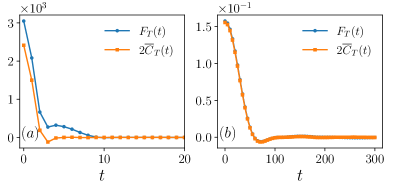
Figure 4: $F_{T}(t)$ [Eq. (9)] and $2\overline{C}_{T}(t)$ [Eq. (10)] for ${\cal A}$ with $q=L/2$ and $L=16$, for (a) $T=\tau_{\text{th}}$ and (b) $T=25\tau_{\text{th}}$.

Dynamics of OTOCs. Correlations between ${\cal O}_{mn}^{T}$ also manifest themselves in dynamical properties Brenes2021 . In particular, we consider out-of-time-ordered correlation function, defined within the energy window $|E_{m}-E_{0}|\leq\frac{\pi}{T}$,

$$F_{T}(t)=\text{Tr}[{\cal O}_{c}^{T}(t){\cal O}_{c}^{T}{\cal O}_{c}^{T}(t){\cal O}_{c}^{T}]\ .$$ (9)

Assuming that off-diagonal matrix elements of ${\cal O}_{c}^{T}$ are uncorrelated and that diagonal elements satisfy ETH SuppMat , $F_{T}(t)$ should reduce to $F_{T}(t)\simeq 2\overline{C}_{T}(t)$, where $\overline{C}_{T}(t)$ is the eigenstate-averaged two-point function,

$$\overline{C}_{T}(t)\equiv\sum_{m=1}^{d}\Re\ \langle m|{\cal O}^{T}_{c}(t){\cal O}^{T}_{c}|m\rangle^{2}\ .$$ (10)

In Fig. 4, $F_{T}(t)$ and $\overline{C}_{T}(t)$ are shown for the density-wave operator ${\cal A}$ with $q=L/2$. We consider $L=16$ and two different energy windows, $T=\tau_{\text{th}}$ [Fig. 4 (a)] and $T=25\tau_{\text{th}}$ [Fig. 4 (b)]. In the former case, we find $F_{T}(t)\neq 2\overline{C}_{T}(t)$, which is consistent with our earlier observation that $\Lambda^{T}\neq 0.5$ at $T=\tau_{\text{th}}$ [Fig. 2 (a)] and supports our conclusion that higher-order correlations exist between the ${\cal O}_{mn}^{T}$. In contrast, in the latter case, $F_{T}(t)\approx 2\overline{C}_{T}(t)$, consistent with $\Lambda^{T}\to 0.5$ and signaling that correlations between the ${\cal O}_{mn}^{T}$ vanish and strict GOE behavior emerges for such narrow energy windows.

Conclusion & Outlook. We have studied presence of correlations between matrix elements of observables written in the energy eigenbasis of chaotic quantum many-body systems. We introduced a novel numerical method to evaluate higher moments of operator submatrices for system sizes beyond those accessible by ED. As a main result, we have shown that even for narrow energy windows, corresponding to time scales of the order of thermalization time for the given observable, matrix elements remain correlated. Consistent with the results of Dymarsky2018 ; Richter2020 , our findings suggest that even though usual indicators of the ETH might be completely fulfilled SuppMat , ETH has to be refined to properly describe all dynamical aspects of thermalization. Specifically, in addition to the usual thermalization or Thouless time controlling RMT behavior of energy levels, there exists another relevant time $T_{\text{RMT}}\gg\tau_{\text{th}}$, which marks the end of macroscopic thermalization dynamics (see also Dymarsky2018 ) and the scale where ${\cal O}_{mn}^{T}$ become uncorrelated. We demonstrated this fact by studying suitably defined OTOCs, which visualized the presence of correlations between ${\cal O}_{mn}^{T}$ well beyond the thermalization time of the two-point function.

A natural next step is to systematically study $L$ dependence of $T_{\text{RMT}}/\tau_{\text{th}}$ for various operators and to clarify the role of conservation laws giving rise to hydrodynamic behavior at late times. While we expect that our findings can be generalized to other systems, it would be interesting to study $T_{\text{RMT}}$ in a wider class of models, including time-dependent Floquet models without energy conservation, as well as disordered systems which may exhibit subdiffusive transport or localization depending on the disorder strength Gopa20 . Finally, another direction is to consider few-body systems with classically chaotic counterpart and to explore $T_{\text{RMT}}$ and its deviations from the Thouless time from a semiclassical point of view.

Acknowledgements. This work has been funded by the Deutsche Forschungsgemeinschaft (DFG), Grants No. 397107022 (GE 1657/3-2), No. 397067869 (STE 2243/3-2), and No. 355031190, within the DFG Research Unit FOR 2692. J. R. has been funded by the European Research Council (ERC) under the European Union’s Horizon 2020 research and innovation programme (Grant agreement No. 853368). A. D. acknowledges support of the Russian Science Foundation (Project No. 17-12-01587).

I Supplemental material

II Evaluation of $\Lambda^{T}$ for matrices with uncorrelated elements

In the main text, we have introduced $\Lambda^{T}={\cal M}_{2}^{2}/{\cal M}_{4}$ [Eq. (3)] as an indicator for the onset of “random-matrix behavior” ($\Lambda^{T}\to 0.5$), in the sense that the operator submatrix ${\cal O}^{T}$ within an energy window of width $2\pi/T$ is well described by a random matrix drawn for instance from a Gaussian Orthogonal Ensemble (GOE) and, in particular, that the matrix elements ${\cal O}_{mn}^{T}$ can be regarded as uncorrelated random numbers. Here, we provide more details on why $\Lambda^{T}$ is indeed a useful quantity even if the matrix is not an instance of a GOE and how to nevertheless interpret the possible outcomes $\Lambda^{T}\neq 0.5$ or $\Lambda^{T}\to 0.5$.

To begin with, we note that for physical operators fulfilling the ETH [Eq. (1) in main text], the variances of off-diagonal matrix elements $|{\cal O}_{mn}|^{2}$ typically decay rapidly with energy distance $\omega$ as described by the envelope function $f(\bar{E},\omega)$, except for a narrow region around the diagonal where $f(\bar{E},\omega)$ is approximately constant. For small $T$, i.e., large energy windows, the submatrices ${\cal O}^{T}$ therefore probe a region where $f(\bar{E},\omega)$ is non-constant and therefore ${\cal O}_{mn}^{T}$ is trivially not described by a GOE, see also Fig. S3 below. Thus, one might expect that even if the $r_{mn}$ in Eq. (1) are uncorrelated random numbers, the level density of ${\cal O}^{T}$ can differ from a semicircle and $\Lambda^{T}$ can deviate from the GOE value $\Lambda^{T}_{\text{GOE}}=0.5$.

For small system sizes $L$, which are accessible by full exact diagonalization, we have demonstrated in Fig. 1 in the main text that it is insightful to compare ${\cal O}_{mn}^{T}$ with a sign-randomized version $\widetilde{\cal O}^{T}_{mn}$ [see Eq. (7) in main text]. In particular, while we find $\Lambda^{T}\neq 0.5$ for ${\cal O}^{T}$ and small $T$, the sign-randomized operator $\widetilde{{\cal O}}^{T}$ in contrast yields the GOE value $\Lambda^{T}=0.5$, indicating that matrix elements ${\cal O}_{mn}^{T}$ exhibit correlations that are destroyed due to the sign-randomization. For larger $L$, for which we have to rely on the typicality approach, such a comparison is not possible anymore. Nevertheless, as we will show in the following, the emergence of $\Lambda^{T}=0.5$ crucially does not depend on $f(\bar{E},\omega)=\text{const.}$, but can be derived solely by assuming that the $r_{mn}$ are uncorrelated and by imposing some mild conditions on the matrix structure of ${\cal O}^{T}$.

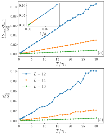
Figure S1: (a) $\frac{1}{d}\sum_{mn}|{\cal O}_{mn}^{T}|^{4}/{\cal M}^{2}_{2}$ versus $T/\tau_{\text{th}}$ and (b) $\sigma_{\cal F}^{2}/{\cal M}^{2}_{2}$ versus $T/\tau_{\text{th}}$ for ${\cal A}$ with $q=\frac{L}{2}$, obtained for the Ising model of the main text and system sizes $L=12,14,16$. Inset in (a) shows $\frac{1}{d}\sum_{mn}|{\cal O}_{mn}^{T}|^{4}/{\cal M}^{2}_{2}$ versus $1/d$.

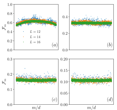
Figure S2: ${\cal F}_{m}$ for the density-wave operator ${\cal A}(q=\frac{L}{2})$ in the Ising model of the main text with $L=12,14,16$. Data is obtained in energy windows $\Delta E=2\pi/T$ with (a) $T=0.5\tau_{\text{th}}$, (b) $T=1\tau_{\text{th}}$, (c) $T=2\tau_{\text{th}}$, (d) $T=3\tau_{\text{th}}$.

To this end, let us write the fourth moment ${\cal M}_{4}$ in the energy basis,

$${\cal M}_{4}=\frac{1}{d}\sum_{mnkl}({\cal O}_{c}^{T})_{mn}({\cal O}_{c}^{T})_{nk}({\cal O}_{c}^{T})_{kl}({\cal O}_{c}^{T})_{lm}\ .$$ (S1)

Assuming that the elements $({\cal O}^{T}_{c})_{mn}$ are uncorrelated, only the “square” terms in the summation of Eq. (S1) are non-negligible. Thus, one gets (we omit the subscript $c$ in ${\cal O}_{c}^{T}$ for simplicity in the following),

$${\cal M}_{4} =\frac{1}{d}\sum_{mnl}|{\cal O}_{mn}^{T}|^{2}|{\cal O}_{lm}^{T}|^{2}+\frac{1}{d}\sum_{mnk}|{\cal O}_{mn}^{T}|^{2}|{\cal O}_{kn}^{T}|^{2}$$

$$\quad-\frac{1}{d}\sum_{mn}|{\cal O}_{mn}^{T}|^{4}$$

$$=\frac{2}{d}\sum_{m}(\sum_{n}|{\cal O}_{mn}^{T}|^{2})^{2}-\frac{1}{d}\sum_{mn}|{\cal O}_{mn}^{T}|^{4}$$

$$=\frac{2}{d}\sum_{m}{\cal F}_{m}^{2}-\frac{1}{d}\sum_{mn}|{\cal O}_{mn}^{T}|^{4}\ ,$$

where we have introduced,

$${\cal F}_{m}=\sum_{n}|{\cal O}_{mn}^{T}|^{2}=\langle m|({\cal O}^{T})^{2}|m\rangle\ ,$$ (S2)

which will play a central role in the following. Let us further introduce the averages,

$$\langle{\cal F}\rangle=\frac{1}{d}\sum_{m}{\cal F}_{m}\ ,\quad\langle{\cal F}^{2}\rangle=\frac{1}{d}\sum_{m}{\cal F}^{2}_{m}\ ,$$ (S3)

and the variance,

$$\sigma^{2}_{\cal F}=\frac{1}{d}\sum_{m}({\cal F}_{m}-\langle{\cal F}\rangle)^{2}\ .$$ (S4)

Then we can write,

$${\cal M}_{4} =2\langle{\cal F}^{2}\rangle-\frac{1}{d}\sum_{mn}|{\cal O}_{mn}^{T}|^{4}\$$

$$=2\langle{\cal F}\rangle^{2}+2\sigma^{2}_{\cal F}-\frac{1}{d}\sum_{mn}|{\cal O}_{mn}^{T}|^{4}$$

$$=2{\cal M}_{2}^{2}+2\sigma^{2}_{\cal F}-\frac{1}{d}\sum_{mn}|{\cal O}_{mn}^{T}|^{4}\ ,$$ (S5)

where we used $\langle{\cal F}\rangle^{2}={\cal M}_{2}^{2}$. Substituting Eq. (S5) into the definition of $\Lambda^{T}$ yields

$$\Lambda^{T} =\frac{{\cal M}_{2}^{2}}{{\cal M}_{4}}=\frac{{\cal M}_{2}^{2}}{2{\cal M}_{2}^{2}+2\sigma_{{\cal F}}^{2}-\frac{1}{d}\sum_{mn}|{\cal O}_{mn}^{T}|^{4}}$$

$$\simeq 0.5-\left(\frac{\sigma_{{\cal F}}^{2}}{2{\cal M}_{2}^{2}}-\frac{\frac{1}{d}\sum_{mn}|{\cal O}_{mn}^{T}|^{4}}{4{\cal M}_{2}^{2}}\right)\ .$$ (S6)

So far, we only assumed that the ${\cal O}_{mn}^{T}$ are uncorrelated. In the following, we will demonstrate that the expressions in the bracket of Eq. (S6) will be negligibly small under reasonably mild requirements on the matrix structure of ${\cal O}^{T}$. First of all, as we consider central moments here, the variance of the diagonal and off-diagonal elements of ${\cal O}^{T}$ should be of the same order if $T$ is sufficiently large and ${\cal O}^{T}$ satisfies ETH. (For the density wave operator that we mainly focus in the main text, this is always the case even if $T$ is quite small.) As a consequence,

$$\frac{\frac{1}{d}\sum_{mn}|{\cal O}_{mn}^{T}|^{4}}{{\cal M}_{2}^{2}}\propto\frac{1}{d}\ ,$$ (S7)

which can therefore be neglected in the case of large $d$. We demonstrate this fact numerically in Fig. S1 (a). In particular, we find that the left hand side of Eq. (S7) is indeed quite small for $L=16$ and scales as $1/d$.

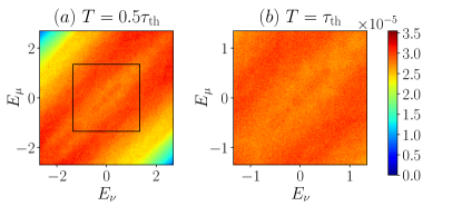
Figure S3: Coarse grained matrix representation of ${\cal A}(q=L/2)$ in the eigenbasis of ${\cal H}$, i.e., averaged squared matrix elements in bins of width $\Delta_{\text{bin}}$, $\frac{1}{\Delta_{\textrm{bin}}^{2}}\sum\limits_{m=\mu}^{\mu+\Delta_{\textrm{bin}}}\sum\limits_{n=\nu}^{\nu+\Delta_{\textrm{bin}}}|\braket{m}{{\cal A}}{n}|^{2}$. Data is shown for $L=16$ in two different energy windows $\Delta E=\frac{\pi}{T}$ with (a) $T=\tau_{\textrm{th}}/2$ and (b) $T=\tau_{\textrm{th}}$. The box in (a) indicates the energy window shown in (b). Note that this data can be interpreted as a visualization of the squared function $f^{2}(\bar{E},\omega)$ in the ETH ansatz.

Secondly, we consider the quantity ${\cal F}_{m}$ introduced in Eq. (S2). In particular, if we assume that ${\cal O}^{T}$ obeys a certain stiffness in the sense that ${\cal F}_{m}$ does not depend strongly on $m$, the variance $\sigma_{\cal F}^{2}$ will be small such that,

$$\frac{\sigma_{{\cal F}}^{2}}{{\cal M}^{2}_{2}}\ll 1\ .$$ (S8)

As demonstrated in Fig. S1 (b), we find that this condition is indeed well fulfilled for the models and operators considered here and that $\sigma_{{\cal F}}^{2}/{\cal M}^{2}_{2}$ quickly decreases with increasing system size. Moreover, in Fig. S2, we plot ${\cal F}_{m}$ for exemplary energy windows $\Delta E=\frac{2\pi}{T}$, emphasizing that fluctuations decrease with increasing $L$ and are already quite small even in energy windows corresponding to $T=\tau_{\text{th}}$.

Combining Eqs. (S6), (S7), and (S8), one thus finds,

$$\Lambda^{T}\simeq 0.5\ ,$$ (S9)

which is just the prediction of the Wigner semicircle spectrum. Let us stress that deriving Eq. (S9) only required that matrix elements are uncorrelated and, as a main assumption, that the fluctuations of ${\cal F}_{m}$ are small. In particular ${\cal O}_{mn}^{T}$ not necessarily have to follow a strict GOE in the sense that $f(\bar{E},\omega)$ can vary within the chosen energy window. This also explains why the sign-randomized operator yields the random-matrix value $\Lambda^{T}=0.5$ even for small $T$ (see Fig. 1 in main text), where $f(\bar{E},\omega)$ is non-constant (see Fig. S3). While we cannot prove that $\sigma_{\cal F}$ will stay small also for system sizes beyond the ones studied in Figs. S1 and S2, we think that this is a reasonable assumption. Thus, $\Lambda^{T}\to 0.5$ remains a meaningful indicator for the emergence of uncorrelated matrix elements, the exploration of which is a main goal of this work.

III Level-spacing statistics of operator submatrices

Let us present additional data supporting that $\Lambda^{T}$ is indeed a very useful and sensitive indicator for the presence of correlations between matrix elements. To this end, let us study another very common “random-matrix indicator”, i.e., the mean ratio $\langle r_{T}\rangle$ of the adjacent level spacings Oganesyan2007S ,

$$\langle r_{T}\rangle=\frac{1}{d}\sum_{\alpha}\frac{\min(\Delta_{\alpha},\Delta_{\alpha+1})}{\max(\Delta_{\alpha},\Delta_{\alpha+1})},$$ (S10)

where $\Delta_{\alpha}=|\lambda^{T}_{\alpha+1}-\lambda^{T}_{\alpha}|$ denotes the gap between two adjacent eigenvalues $\lambda^{T}_{\alpha}$ of ${\cal O}^{T}$, and the averaging is performed over all the gaps in the energy window. For a random matrix drawn from the GOE, $r_{\text{GOE}}\approx 0.53$, while for the uncorrelated Poisson distributed eigenvalues, one finds $r_{\text{Poisson}}\approx 0.39$. As can be seen from Fig. S4, for both operators ${\cal A}(q=L/2)$ and ${\cal A}(q=1)$, we find that $\langle r_{T}\rangle$ is close to the GOE value for the entire range of $T$ shown here. In this context, let us stress that our comparison with the sign-randomized operator in Fig. 1 in the main text has unveiled that the matrix elements of ${\cal O}^{T}$ clearly exhibit correlations at small $T$, manifest in a value $\Lambda^{T}\neq 0.5$. In contrast, as demonstrated in Fig. S4, $\langle r_{T}\rangle$ is not sensitive to this transition from correlated to uncorrelated matrix elements with increasing $T$.

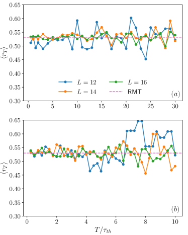
Figure S4: Mean adjacent gap ratio $\langle r_{T}\rangle$ for the density wave operator ${\cal A}$ with (a) $q=L/2$ and (b) $q=1$, obtained within different energy window $\Delta E=2\pi/T$ and system sizes $L=12,14,16$ for the Ising model ${\cal H}$ of the main text.

IV Reduction of OTOC to two-point correlation functions

Let us provide details on the relation $F_{T}(t)\approx 2\overline{C}_{T}(t)$ valid in case matrix elements of ${\cal O}_{c}^{T}$ are uncorrelated, which we used in the context of Fig. 4 in the main text. In the energy eigenbasis, the out-of-time-ordered correlator $F_{T}(t)$ can be written as,

$$F_{T}(t)=\sum_{mnkl}{\cal O}_{mn}^{T}{\cal O}_{nk}^{T}{\cal O}_{kl}^{T}{\cal O}_{lm}^{T}e^{-i(E_{n}-E_{m}+E_{l}-E_{k})t}.$$ (S11)

Assuming that matrix elements ${\cal O}^{T}_{mn}$ are uncorrelated, as well as the variances of the diagonal and off-diagonal elements of ${\cal O}^{T}_{c}$ are of same order, one finds (see also Brenes2021S ),

$$F_{T}(t) \simeq\sum_{m}\sum_{n}|{\cal O}_{mn}^{T}|^{2}e^{-i(E_{n}-E_{m})t}\sum_{l}|{\cal O}_{ml}^{T}|^{2}e^{-i(E_{l}-E_{m})t}$$

$$+\sum_{n}\sum_{m}|{\cal O}_{nm}^{T}|^{2}e^{-i(E_{n}-E_{m})t}\sum_{l}|{\cal O}_{nk}^{T}|^{2}e^{-i(E_{n}-E_{k})t}$$

$$=\sum_{m}(\sum_{n}|{\cal O}_{mn}^{T}|^{2}e^{-i(E_{n}-E_{m})t})^{2}+c.c.$$

$$=2\sum_{m}\Re\left((\langle m|{\cal O}^{T}(t){\cal O}^{T}|m\rangle)^{2}\right)$$

$$=2\overline{C}_{T}(t)\ .$$ (S12)

where we used arguments similar to Eq. (S1) above.

V Details on the numerical approach

In this section, we provide more details on our numerical approach, based on quantum typicality, which is used to simulate the random-matrix indicator $\Lambda^{T}$ and the dynamical correlation function $C(t)$.

V.1 Implementing the energy filter and calculating $\Lambda^{T}$

To begin with, it is useful to rewrite $\exp[-i({\cal H}-E_{0})t]$ as

$$\exp(-i({\cal H}-E_{0})t)=\exp(-i(b-E_{0})t)\exp(-iat\frac{{\cal H}-b}{a}),$$ (S13)

where the second term can be expanded in terms of Chebyshev polynomials of the first kind [denoted by $T_{k}(x)$],

$$\exp(-iat\frac{{\cal H}-b}{a})=J_{0}(at)+2\sum_{k=1}^{\infty}(-i)^{k}J_{k}(at)T_{k}(\frac{{\cal H}-b}{a})\ ,$$ (S14)

where $a=(E_{\text{max}}-E_{\text{min}})/2$, $b=(E_{\text{max}}+E_{\text{min}})/2$, and $J_{k}$ are Bessel functions of the first kind and order $k$. Substituting Eqs. (S13) and (S14) into the definition of $P_{T}$ in the main text, one has

$$P_{T} =\frac{1}{T}\int_{-\infty}^{+\infty}\text{sinc}(\frac{t}{T})\exp(-i({\cal H}-E_{0})t)dt$$ (S15)

$$=\frac{1}{T}\int_{-\infty}^{+\infty}\text{sinc}(\frac{t}{T})\exp(-i(b-E_{0})t)$$

$$\cdot\left[J_{0}(at)T_{0}(\frac{{\cal H}-b}{a})+2\sum_{k=1}^{\infty}(-i)^{k}J_{k}(at)T_{k}(\frac{{\cal H}-b}{a})\right]dt\ .$$ (S16)

After calculating the integral in Eq. (S16) analytically , one gets

$$P_{T}=\sum_{k=0}^{\infty}C_{k}T_{k}(\frac{{\cal H}-b}{a})\ ,$$ (S17)

where

$$C_{0}=\frac{1}{\pi}\left(\frac{\arcsin(\frac{\pi}{T}+b-E_{0})}{a}-\frac{\arcsin(-\frac{\pi}{T}+b-E_{0})}{a}\right)\ ,$$ (S18)

and

$$C_{k}(k\geq 1) =\frac{2(-1)^{k+1}}{\pi k}\biggl{[}\sin\biggl{(}k\arccos\biggl{(}\frac{\frac{\pi}{T}+b-E_{0}}{a}\biggl{)}\biggl{)}$$

$$-\sin\biggl{(}k\arccos\biggl{(}\frac{-\frac{\pi}{T}+b-E_{0}}{a}\biggl{)}\biggl{)}\biggl{]}\ ,$$ (S19)

under the condition

$$-a+b+\frac{\pi}{T}\leq E_{0}\leq a+b-\frac{\pi}{T}\ ,$$ (S20)

which is always fulfilled in our simulations as we only consider the middle region of the spectrum.

In order to study Eq. (S17) numerically, we consider only a finite number of terms in the summation,

$$P_{T}=\sum_{k=0}^{M}C_{k}T_{k}(\frac{{\cal H}-b}{a})\ .$$ (S21)

In our numerical simulations, we choose $M=6aT$, which yields quite accurate values for $\Lambda^{T}$, but is still low enough such that numerical costs remain reasonable. This is demonstrated in Fig. S5, where we compare the results of two different choices of $M$, $M=6aT$ and $M=10aT$. We find that the results are very similar and agree convincingly with the data obtained by exact diagonalization.

In our numerical approach, we calculate the moments ${\cal M}_{k}$ by making use of quantum typicality Jin2021S ; Heitmann2020S , where the energy filter $P_{T}$ is applied to a random pure quantum state. The variance of the statistical error within this approach scales as $1/d$, where $d$ is the effective dimension of the Hilbert space, i.e., the number of eigenstates within the energy window. For a fixed $\Delta E$, our approximation becomes more accurate for larger system size $L$, as $d$ usually scales exponentially with $L$. Even for moderate system sizes, one can improve the accuracy by averaging over $N$ different realizations of random states, which can reduce the variance by a factor $N$. In our numerical simulations, $N$ is adjusted as a function of system $L$, $N\propto\frac{1}{2^{L}}$, yielding accurate results for all system sizes considered by us.

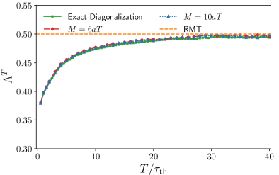
Figure S5: $\Lambda^{T}$ versus $T/\tau_{\text{th}}$ for ${\cal A}(q=L/2)$ and system size $L=16$ in Ising model. Results are obtained by the typicality approach, averaged over 500 states, for two different value of $M=6aT$ (red) and $M=10aT$ (blue).

V.2 Details on the typicality approach for the autocorrelation function

Given the operator ${\cal O}$, the its infinite-temperature autocorrelation function can be studied with quantum typicality as,

$$C(t)=\text{Tr}[{\cal O}(t){\cal O}]/2^{L}\simeq\langle\psi|{\cal O}(t){\cal O}|\psi\rangle\ ,$$ (S22)

where $|\psi\rangle$ is a pure state drawn at random from the unitarily invariant Haar measure, and $\braket{\psi}{\psi}=1$. Introducing an auxiliary state $|\psi_{\cal O}\rangle={\cal O}|\psi\rangle$, Eq. (S22) can be written as,

$$C(t)\simeq\langle\psi(t)|{\cal O}|\psi_{\cal O}(t)\rangle,$$ (S23)

where

$$|\psi(t)\rangle=\exp(-i{\cal H}t)|\psi\rangle,\quad|\psi_{\cal O}(t)\rangle=\exp(-i{\cal H}t)|\psi_{\cal O}\rangle\ ,$$ (S24)

which can be efficiently simulated by means of sparse-matrix techniques.

It is well established that the error of the typicality approximation (S23) decreases exponentially for increasing system size Heitmann2020S . While this error becomes negligibly small for the larger values of $L$ considered by us, it can again be reduced for smaller $L$ by averaging over different realizations of random states. We demonstrate the accuracy of quantum typicality in Fig. S6, where we compare the dynamics obtained by quantum typicality (averaged over $1000$ random states) with exact diagonalization data for the Ising model ${\cal H}$ with $L=16$. For both operators ${\cal A}(q=1)$ and ${\cal A}(q=L/2)$ considered here, we find that the typicality approach is very accurate, even at long times around $\tau_{\text{th}}$, where $C(t)$ has decayed for rather small values.

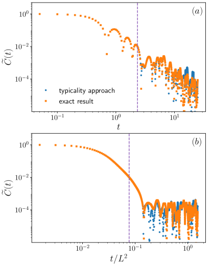
Figure S6: Exact results of rescaled autocorrelation function $\widetilde{C}(t)$ versus data obtained by quantum typicality (averaged over 1000 random states) for (a) ${\cal A}(q=1)$ and (b) ${\cal A}(q=L/2)$ in the Ising model ${\cal H}$ with $L=16$. The dashed line signals the thermalization time $\tau_{\text{th}}$ according to our definition in the main text.

VI Usual indicators of the ETH and quantum chaos

Let us demonstrate that the operators considered in the main text are in good agreement with standard indicators of the ETH.

VI.1 Diagonal matrix elements

As a first step, we study the diagonal part of the ETH. To this end, Fig. S7 shows the matrix elements $\langle m|{\cal A}|m\rangle$ and $\langle m|{\cal B}|m\rangle$, for different system sizes $L=12,14,16$ in the Ising model. For energy densities in the center of the spectrum, we find that the “cloud” of matrix elements becomes narrower with increasing $L$, which is in good accord with the ETH prediction that the ${\cal O}_{mm}$ should form a “smooth” function of energy in the thermodynamic limit $L\rightarrow\infty$, and that the fluctuation of ${\cal O}_{mm}$ decay exponentially with $L$.

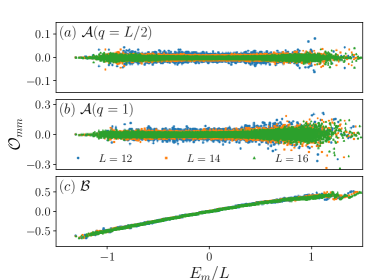
Figure S7: Diagonal matrix elements of operators (a) ${\cal A}(q=L/2)$, (b) ${\cal A}(q=1)$, and (c) ${\cal B}$, in the eigenbasis of the Ising model $\cal H$ with $L=12,14,16$ .

VI.2 Off-diagonal matrix elements

We now turn to the properties of the off-diagonal matrix elements ${\cal O}_{mn}$, where we focus on the eigenstates with mean energy $\bar{E}\in[-0.5,0.5]$. Assuming the ${\cal O}_{mn}$ have zero mean, i.e. $\overline{{\cal O}_{mn}}=0$, (which we find to hold to a very high accuracy), we study the frequency-dependent ratio $\Gamma(\omega)$, recently introduced in Ref. LeBlond2019S ,

$$\Gamma(\omega)=\frac{\overline{|{\cal O}_{mn}|^{2}}(\omega)}{[\overline{|{\cal O}_{mn}|}(\omega)]^{2}}\ ,$$ (S25)

where,

$$\overline{|{\cal O}_{mn}|^{2}}(\omega) =\frac{1}{N_{\omega}}\sum_{\begin{subarray}{c}m,n\\ |E_{m}-E_{m}|\approx\omega\end{subarray}}|{\cal O}_{mn}|^{2}\ ,$$ (S26)

$$\overline{|{\cal O}_{mn}|}(\omega) =\frac{1}{N_{\omega}}\sum_{\begin{subarray}{c}m,n\\ |E_{m}-E_{m}|\approx\omega\end{subarray}}|{\cal O}_{mn}|\ .$$ (S27)

Here the sum runs over all $N_{\omega}$ matrix elements with $|E_{m}-E_{n}|\in|\omega-\Delta\omega/2,\omega+\Delta\omega/2|$, where we choose $\Delta\omega=0.05$ in our numerical simulation. In Fig. S8 we find that $\Gamma(\omega)$ is close to the Gaussian value $\pi/2$ for almost all values of $\omega$ and $L$ considered here, indicating a Gaussian distribution of ${\cal O}_{mn}$.

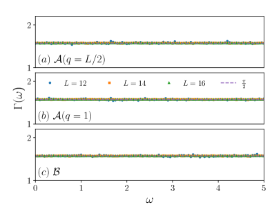
Figure S8: $\Gamma(\omega)$ for matrix elements of operator (a) ${\cal A}(q=L/2)$, (b) ${\cal A}(q=1)$, (c) ${\cal B}$, in the energy window $\overline{E}\in[-0.5,0.5]$ and system sizes $L=12,14,16$ in Ising model.

Furthermore, we also calculate the ratio $\Sigma^{2}(n,\mu)$ dalessio2016S ; Mondaini2017S ; jansen2019S between the variances of diagonal and off-diagonal matrix elements for eigenstates in regions $[n-\mu/2,n+\mu/2]$ of width $\mu$ (see also Richter2020S ),

$$\Sigma^{2}(n,\mu)=\frac{\sigma^{2}_{\text{d}}(n,\mu)}{\sigma^{2}_{\text{od}}(n,\mu)}\ .$$ (S28)

In Figs. S9 (a) and S9 (b), we study the ratio $\Sigma^{2}(n,\mu)$ of the density-wave operator ${\cal A}$ for $q=L/2$ and $q=1$, respectively. Specifically, the data are obtained for $L=16$ with two different square sizes $\mu=100,1000$ and all possible embedding along the diagonal of the submatrix with dimension ${\cal D}^{\prime}\approx{\cal D}/2$, where ${\cal D}=2^{L}$ is the total dimension of the Hilbert space. We observe that $\Sigma^{2}(n,\mu)$ fluctuates around the GOE prediction $\Sigma^{2}_{\text{GOE}}=2$.

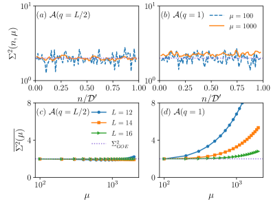
Figure S9: [(a),(b)] Ratio $\Sigma^{2}(n,\mu)$ between the variances of diagonal and off-diagonal matrix elements for two different square sizes $\mu=100,1000$ and all embeddings $n\in[1+\mu/2,{\cal D}^{\prime}-\mu/2]$ for operator ${\cal A}$ in Ising model. The data are obtained for system size $L=16$ and the dashed line indicates the RMT prediction $\Sigma^{2}_{\text{GOE}}=2$. [(c),(d)] Average value $\overline{\Sigma^{2}(\mu)}$ versus $\mu$ for system sizes $L=12,14,16$. Panels (a) and (c) show data for $q=L/2$, while (b) and (d) show data for $q=1$.

In Figs. S9 (c) and S9 (d), we show the averaged value

$$\overline{\Sigma^{2}(\mu)}=\frac{1}{{\cal D}^{\prime}-\mu}\sum_{n=1+\mu/2}^{{\cal D}^{\prime}-\mu/2}\Sigma^{2}(n,\mu)\ .$$ (S29)

We find that $\overline{\Sigma^{2}(\mu)}\approx\Sigma^{2}_{\text{GOE}}$ for small $\mu$, while it grows monotonously with increasing $\mu$ [this growth is particularly pronounced in the case of slowest mode $q=1$ as shown in Fig. S9 (d)]. Comparing the results for different $L$, we find that $\overline{\Sigma^{2}(\mu)}$ remains closer to $\Sigma^{2}_{\text{GOE}}$ for larger $L$, and it is reasonable to expect that $\overline{\Sigma^{2}(\mu)}\approx\Sigma^{2}_{\text{GOE}}$ holds in the thermodynamic limit $L\rightarrow\infty$, indicating ${\cal O}_{mn}$ follow a Gaussian distribution, at least for $m,n$ in the middle of the energy spectrum.

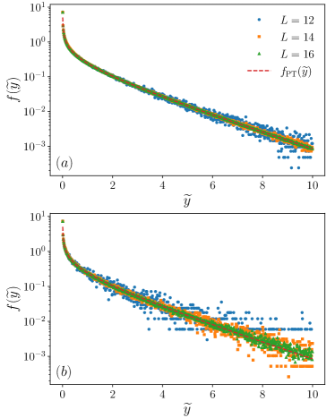
Figure S10: Distribution of rescaled transition strength $\widetilde{y}$ for (a) ${\cal A}(q=L/2)$ and (b) ${\cal A}(q=1)$ within the energy window $[-\pi/\tau_{\text{th}},\pi/\tau_{\text{th}}]$. Data is obtained for the Ising model ${\cal H}$ with $L=12,14,16$. The dashed line indicates the Porter-Thomas distribution, which is predicted by GOE.

Eventually, we also study the distribution of the transition strengths, taking $\cal A$ with $q=L/2$ and $q=1$ as probe operators. More specifically, we consider $y={\cal A}^{2}_{mn}$, which should follow the Porter-Thomas distribution P-T , if the matrix elements are drawn according to a GOE. In Fig. S10, we take into account the matrix elements ${\cal A}^{2}_{mn}$ within the energy window $E_{m},E_{n}\in[-\pi/\tau_{\text{th}},\pi/\tau_{\text{th}}]$, and study the distribution of the rescaled transition strength $\widetilde{y}={\cal A}^{2}_{mn}/\langle{\cal A}^{2}_{mn}\rangle$ [denoted by $f(\widetilde{y})$]. One can see that $f(\widetilde{y})$ can be well described by the Porter Thomas distribution (which is also the $\chi^{2}$ distribution with one degree of freedom)

$$f_{\text{PT}}(\widetilde{y})=(2\pi)^{-1/2}\widetilde{y}^{-1/2}\exp(-\widetilde{y}/2),$$ (S30)

for both operators and all system sizes considered here.

VII Numerical results of $\Lambda^{T}$ in XXZ model

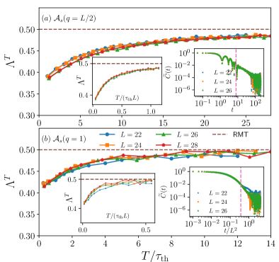
Figure S11: $\Lambda^{T}$ versus $T/\tau_{\text{th}}$ for the spin density-wave operator ${\cal A}_{s}$ (S32) in XXZ model (described by ${\cal H}_{2}$) with (a) $q=L/2$ and (b) $q=1$. Data is obtained using typicality approach, averaged over $500\cdot 2^{L-18}$ states, for up to $L=28$. The dashed horizontal line indicates the GOE value $\Lambda^{T}=0.5$. The two insets show $\Lambda^{T}$ versus $T/(\tau_{\text{th}}L)$ and the rescaled autocorrelation function $\widetilde{C}(t)$ in log-log scale, obtained by typicality approach. The dashed vertical line signals the thermalization time $\tau_{\text{th}}$ according to our definition. Good quality of collapse of $C(t)$ and $C(t/L^{2})$ correspondingly for different $L$ confirms $L$-independence of $\tau_{\text{th}}$ for $q=L/2$ and diffusive behavior $\tau_{\text{th}}\propto L^{2}$ for $q=1$.

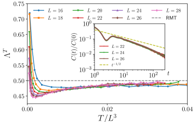
Figure S12: $\Lambda^{T}$ versus $T/\tau_{\text{th}}$ for local operator $s_{z}^{\lfloor\frac{L}{2}\rfloor}$ in XXZ model ${\cal H}_{3}$. Data for $L=16$ is obtained by exact diagonalization, while data for $L\geq 18$ is obtained by our typicality approach, averaged over $500\cdot 2^{L-18}$ states. The dashed horizontal line indicates the RMT value $\Lambda^{T}=0.5$. The inset shows the autocorrelation function $C(t)$, normalized by its initial value, where the dashed line indicates a $t^{-1/2}$ decay.

In addition to the Ising model studied in the main text, we also consider a nonintegrable XXZ model with next-nearest neighbor interactions,

$${\cal H}_{2} =\sum_{\ell=1}^{L}s_{x}^{\ell}s_{x}^{\ell+1}+s_{y}^{\ell}s_{y}^{\ell+1}+\Delta_{1}s_{z}^{\ell}s_{z}^{\ell+1}$$

$$+\sum_{\ell=1}^{L}\Delta_{2}s_{z}^{\ell}s_{z}^{\ell+2}+h_{1}s_{z}^{1}+h_{\lfloor\frac{L}{3}\rfloor+1}s_{z}^{\lfloor\frac{L}{3}\rfloor+1}\ ,$$ (S31)

where $s^{\ell}_{x,y,z}=\frac{1}{2}\sigma^{\ell}_{x,y,z}$ are spin operators at lattice site $\ell$, $L$ is the length of the chain with periodic boundaries, and we choose $\Delta_{1}=1.5,\Delta_{2}=0.5,h_{1}=0.1,h_{\lfloor\frac{L}{3}\rfloor+1}=0.075$ ($\lfloor\rfloor$ indicates the floor function). The two defects are added to lift the translation and reflection symmetries. The zero magnetization subspace is considered and the energy center is chosen to be $E_{0}=-0.3L/16$, corresponding to infinite temperature. We consider a spin density-wave operator,

$${\cal A}_{s}=\sum_{\ell=1}^{L}\cos(\frac{2\pi}{L}\ell q)s_{z}^{\ell}\ ,$$ (S32)

which exhibits slow hydrodynamics relaxation in the limit of small $q$.

In Fig. S11, analogous to the results obtained for the the Ising model in the main text, we find that $\Lambda^{T}\neq 0.5$ at small $T$, indicating the presence of correlations between matrix elements. Only at much longer times $T\gg\tau_{\text{th}}$, we observe that $\Lambda^{T}\to 0.5$ suggesting a transition to genuine GOE behavior. Furthermore, by plotting $\Lambda^{T}$ as a function of $T/(\tau_{\text{th}}L)$, the good numerical collapse extending through almost all values of $T$ tentatively suggests $T_{\text{RMT}}\propto\tau_{\text{th}}L$ for ${\cal A}_{s}$ with $q=L/2$, see inset in Fig. S11 (a). Note, however, that such a data collapse is less clear for $q=1$, see inset in Fig. S11 (b).

Finally, in order to connect to the results presented in Ref. Richter2020S , we also consider the next-nearest neighbor XXZ chain with the parameters used in Richter2020S ,

$${\cal H}_{3} =\sum_{\ell=1}^{L}s_{x}^{\ell}s_{x}^{\ell+1}+s_{y}^{\ell}s_{y}^{\ell+1}+\Delta_{1}s_{z}^{\ell}s_{z}^{\ell+1}$$

$$+\sum_{\ell=1}^{L}\Delta_{2}s_{z}^{\ell}s_{z}^{\ell+2}+h_{1}s_{z}^{1},$$ (S33)

namely $h_{1}=0.1,\Delta_{1}=1.5,\Delta_{2}=1.2$, and open boundary conditions. As before, we consider the zero magnetization subspace. Moreover, we study a local operator $s_{z}^{\lfloor\frac{L}{2}\rfloor}$ in the middle of the chain, which exhibits a power-law relaxation (approximately $\propto t^{-1/2}$), see inset in Fig. S12. As shown in in Fig. S12, we find that although a “sharp transition” to RMT seems to exist for small system sizes ($L=16$), the analysis of longer chains unveils that $\Lambda^{T}\to 0.5$ only at times much longer than the thermalization time. Interestingly, we observe a good numerical collapse of all the curves as a function of $T/L^{3}$ (note that $t_{\text{th}}\propto L^{2}$ for this operators), which is consistent with the analytical prediction in Ref. Dymarsky2018S .

References

- (1) A. Polkovnikov, K. Sengupta, A. Silva, and M. Vengalattore, Rev. Mod. Phys. 83, 863 (2011).
- (2) C. Gogolin and J. Eisert, Rep. Prog. Phys. 79, 056001 (2016).
- (3) L. D’Alessio, Y. Kafri, A. Polkovnikov, and M. Rigol, Adv. Phys. 65, 239 (2016).
- (4) F. Borgonovi, F. M. Izrailev, L. F. Santos, and V. G. Zelevinsky, Phys. Rep. 626, 1 (2016).
- (5) T. Mori, T. N. Ikeda, E. Kaminshi, and M. Ueda, J. Phys. B: At. Mol. Opt. Phys. 51, 112001 (2018).
- (6) S. Trotzky, Y.-A. Chen, A. Flesch, I. P. McCulloch, U. Schollwöck, J. Eisert, and I. Bloch, Nat. Phys. 8, 325 (2012).
- (7) A. M. Kaufmann, M. E. Tai, A. Lukin, M. Rispoli, R. Schittko, P. M. Preiss, and M. Greiner, Science 353, 794 (2016).
- (8) J. Choi, H. Zhou, S. Choi, R. Landig, W. W. Ho, J. Isoya, F. Jelezko, S. Onoda, H. Sumiya, D. A. Abanin, and M. D. Lukin, Phys. Rev. Lett. 122, 043603 (2019).
- (9) Y. Tang, W. Kao, K.-Y. Li, S. Seo, K. Mallayya, M. Rigol, S. Gopalakrishnan, and B. L. Lev, Phys. Rev. X 8, 021030 (2018).
- (10) G. Clos, D. Porras, U. Warring, and T. Schaetz, Phys. Rev. Lett. 117, 170401 (2016).
- (11) H. Kim, Y. Park, K. Kim, H.-S. Sim, and J. Ahn, Phys. Rev. Lett. 120, 180502 (2018).
- (12) S. Lepoutre, J. Schachenmayer, L. Gabardos, B. Zhu, B. Naylor, E. Maréchal, O. Gorceix, A. M. Rey, L. Vernac, and B. Laburthe-Tolra, Nat. Commun. 10, 1714 (2019).
- (13) S. Hofferberth, I. Lesanovsky, B. Fischer, T. Schumm, and J. Schmiedmayer, Nature (London) 449, 324 (2007).
- (14) Quantum Chaos: Between Order and Disorder, edited by G. Casati and B.V. Chirikov, (Cambridge University Press, Cambridge, England, 1994).
- (15) F. Haake, S. Gnutzmann, M. Kús, Quantum signatures of chaos, Springer Series in Synergetics (Springer, Cham, 2018).
- (16) V. Zelevinsky, B. A. Brown, M. Horoi, and N. Frazier, Phys. Rep. 276, 85 (1996).
- (17) F. M. Izrailev, Phys. Rep. 196, 299 (1990).
- (18) T. A. Brody, J. Flores, J. B. French, P. A. Mello, A. Pandey, and S. S. M. Wong, Rev. Mod. Phys. 53, 385 (1981).
- (19) T. Guhr, A. Müller-Groeling, and H. A. Weidenmüller, Phys. Rep. 299, 189 (1998).
- (20) Y. Alhassid, Rev. Mod. Phys. 72, 895 (2000).
- (21) C. W. J. Beenakker, Rev. Mod. Phys. 69, 731 (1997).
- (22) J. M. Deutsch, Phys. Rev. A 43, 2046 (1991).
- (23) M. Srednicki, Phys. Rev. E 50, 888 (1994).
- (24) M. Rigol, V. Dunjko, and M. Olshanii, Nature 452, 854 (2008).
- (25) R. V. Jensen and R. Shankar, Phys. Rev. Lett. 54, 1879 (1985).
- (26) M. Feingold and A. Peres, Phys. Rev. A 34, 591 (1986).
- (27) M. Feingold, D. Leitner, and M. Wilkinson, Phys. Rev. Lett. 66, 986 (1991).
- (28) R. Steinigeweg, J. Herbrych, and P. Prelovšek, Phys. Rev. E 87, 012118 (2013).
- (29) W. Beugeling, R. Moessner, and M. Haque, Phys. Rev. E 89, 042112 (2014).
- (30) H. Kim, T. N. Ikeda, D. A. Huse, Phys. Rev. E 90, 052105 (2014).
- (31) E. J. Torres-Herrera and L. F. Santos, Phys. Rev. E 89, 062110 (2014).
- (32) R. Mondaini, K. R. Fratus, M. Srednicki, and M. Rigol, Phys. Rev. E 93, 032104 (2016).
- (33) R. Mondaini and M. Rigol, Phys. Rev. E 96, 012157 (2017).
- (34) D. Jansen, J. Stolpp, L. Vidmar, and F. Heidrich-Meisner, Phys. Rev. B 99, 155130 (2019).
- (35) T. LeBlond, K. Mallayya, L. Vidmar, and M. Rigol, Phys. Rev. E 100, 062134 (2019).
- (36) M. Brenes, T. LeBlond, J. Goold, and M. Rigol, Phys. Rev. Lett. 125, 070605 (2020).
- (37) J. Richter, A. Dymarsky, R. Steinigeweg, and J. Gemmer, Phys. Rev. E 102, 042127 (2020).
- (38) J. D. Noh, Phys. Rev. E 103, 012129 (2021).
- (39) J. Richter, J. Gemmer, and R. Steinigeweg, Phys. Rev. E 99, 050104(R) (2019).
- (40) A. Dymarsky and K. Pavlenko, Phys. Rev. Lett. 123, 111602 (2019).
- (41) K. Kaneko, E. Iyoda, and T. Sagawa, Phys. Rev. A 101, 042126 (2020).
- (42) M. Mierzejewski and L. Vidmar, Phys. Rev. Lett. 124, 040603 (2020).
- (43) M. Brenes, S. Pappalardi, J. Goold, and A. Silva, Phys. Rev. Lett. 124, 040605 (2020).
- (44) M. Serbyn, D. A. Abanin, and Z. Papić, Nat. Phys. 17, 675 (2021).
- (45) G. Casati, L. Molinari, and F. Izrailev, Phys. Rev. Lett. 64, 1851 (1990).
- (46) Y. V. Fyodorov and A. D. Mirlin, Phys. Rev. Lett. 67, 2405 (1991).
- (47) V. K. B. Kota, Phys. Rep. 347, 223 (2001).
- (48) J. B. French and S. S. M. Wong, Phys. Lett. B 33, 449 (1970).
- (49) J. Flores, M. Horoi, M. Müller, and T. H. Seligman, Phys. Rev. E 63, 026204 (2001).
- (50) D. J. Luitz, I. M. Khaymovich, and Y. Bar Lev, SciPost Phys. Core 2, 006 (2020).
- (51) Y. Alhassid and R. D. Levine, Phys. Rev. Lett. 57. 2879 (1986).
- (52) Y. Alhassid and M. Feingold, Phys. Rev. A 39, 374 (1989).
- (53) C. I. Barbosa, T. Guhr, and H. L. Harney, Phys. Rev. E 62, 1936 (2000).
- (54) A. Dymarsky and H. Liu, Phys. Rev. E 99, 010102 (2019).
- (55) S. Hortikar, M. Srednicki, Phys. Rev. E 57, 7313 (1998).
- (56) S. Hortikar, M. Srednicki, Phys. Rev. E 61, R2180(R) (2000).
- (57) B. Eckhardt and J. Main, Phys. Rev. Lett. 75, 2300 (1995).
- (58) A. Dymarsky, arXiv:1804.08626.
- (59) M. Brenes, S. Pappalardi, M. T. Mitchison, J. Goold, and A. Silva, Phys. Rev. E 104, 034120 (2021).
- (60) L. Foini and J. Kurchan, Phys. Rev. E 99, 042139 (2019).
- (61) A. Chan, A. De Luca, and J. T. Chalker, Phys. Rev. Lett. 122, 220601 (2019).
- (62) C. Murthy and M. Srednicki, Phys. Rev. Lett. 123, 230606 (2019).
- (63) B. Swingle, G. Bentsen, M. Schleier-Smith, and P. Hayden Phys. Rev. A 94, 040302(R) (2016).
- (64) J. Cotler, N. Hunter-Jones, J. Liu, and Beni Yoshida, J. High Energ. Phys. 2017, 48 (2017).
- (65) J. Cotler and N. Hunter-Jones, J. High Energ. Phys. 2020, 205 (2020).
- (66) S. Moudgalya, T. Devakul, C. W. von Keyserlingk, and S. L. Sondhi, Phys. Rev. B 99, 094312 (2019).
- (67) M. Schiulaz, E. J. Torres-Herrera, and L. F. Santos, Phys. Rev. B 99, 174313 (2019).
- (68) B. Bertini, F. Heidrich-Meisner, C. Karrasch, T. Prosen, R. Steinigeweg, and M. Žnidarič, Rev. Mod. Phys. 93, 025003 (2021).
- (69) D. A. Abanin, E. Altman, I. Bloch, and M. Serbyn, Rev. Mod. Phys. 91, 021001 (2019).
- (70) D. J. Thouless, Phys. Rep. 13, 93 (1974).
- (71) The thermalization time can be intepreted as a generalization of the original “Thouless time” in the context of transport Thouless1974 , as an excitation takes this time to diffuse across the system, cf. discussion around Eq. (8). The inverse scale marks the frequency below which [Eq. (1)] is approximately constant, sometimes called Thouless energy Serbyn2017 . At the same time, the notion of “Thouless energy” has also been associated with applicability of RMT to the energy spectrum Schiulaz2019 ; Prosen2020 ; Kos2021 ; Moudgalya2021 ; Piotr20 . In some cases, .
- (72) M. Serbyn, Z. Papić, and D. Abanin, Phys. Rev. B 96, 104201 (2017).
- (73) J. Šuntajs, J. Bonča, T. Prosen, L. Vidmar, Phys. Rev. E 102, 062144 (2020).
- (74) P. Kos, B. Bertini, and T. Prosen, Phys. Rev. Lett. 126, 190601 (2021).
- (75) S. Moudgalya, A. Prem, D. A. Huse, and A. Chan, Phys. Rev. Research 3, 023176 (2021).
- (76) P. Sierant, D. Delande, and J. Zakrzewski Phys. Rev. Lett. 124, 186601 (2020).
- (77) F. Jin, D. Willsch, M. Willsch, H. Lagemann, K. Michielsen, and H. De Raedt, J. Phys. Soc. Jpn. 90, 012001 (2021).
- (78) T. Heitmann, J. Richter, D. Schubert, and R. Steinigeweg, Z. Naturforsch. A 75, 421 (2020).
- (79) See supplemental material for details on the meaning of including its analytical evaluation for uncorrelated matrix elements, as well as details on other random-matrix indicators beyond , OTOCs, the accuracy of our typicality approach, additional numerical data on ETH indicators for , and for other models and observables, including Ref. P-TMain .
- (80) C. E. Porter and R. G. Thomas, Phys. Rev. 104, 483 (1956).
- (81) H. Tal-Ezer and R. Kosloff, J. Chem. Phys. 81, 3967 (1984).
- (82) V. V. Dobrovitski and H. De Raedt, Phys. Rev. E 67, 056702 (2003).
- (83) A. Weiße, G. Wellein, A. Alvermann, and H. Fehske, Rev. Mod. Phys. 78, 275 (2006).
- (84) C. Bartsch and J. Gemmer, Phys. Rev. Lett. 102, 110403 (2009).
- (85) In our simulations, we choose , which yields quite accurate values for SuppMat , but is still low enough such that numerical costs remain reasonable.
- (86) Y. Yamaji, T. Suzuki, and M. Kawamura, arXiv:1802.02854.
- (87) S. Garnerone and T. R. de Oliveira, Phys. Rev. B 87, 214426 (2013).
- (88) P. Sierant, D. Delande, and J. Zakrzewski Phys. Rev. Lett. 125, 156601 (2020).
- (89) R. Steinigeweg, A. Khodja, H. Niemeyer, C. Gogolin, and J. Gemmer, Phys. Rev. Lett. 112, 130403 (2014).
- (90) H. Kim and D. A. Huse, Phys. Rev. Lett. 111, 127205 (2013).
- (91) V. Oganesyan and D. A. Huse, Phys. Rev. B 75, 155111 (2007).
- (92) D. Cohen and T. Kottos, Phys. Rev. E 63, 036203 (2001).
- (93) T. Kottos and D. Cohen, Phys. Rev. E 64, 065202(R) (2001).
- (94) T. Elsayed and B. Fine, Phys. Rev. Lett. 110, 070404 (2013).
- (95) is numerically obtained as an average over fluctuations at long times. While the definition of is not unique, our employed criterion remains numerically well controlled for all .
- (96) This leads to small and comparable statistical errors for all considered here.
- (97) T. L. M. Lezama, E. J. Torres-Herrera, F. Pérez-Bernal, Y. Bar Lev, and L. F. Santos, Phys. Rev. B 104, 085117 (2021).
- (98) S. Gopalakrishnan and S. A. Parameswaran, Phys. Rep. 862, 1 (2020).

References

- (1) V. Oganesyan and D. A. Huse, Phys. Rev. B 75, 155111 (2007).
- (2) M. Brenes, S. Pappalardi, M. T. Mitchison, J. Goold, and A. Silva, Phys. Rev. E 104, 034120 (2021).
- (3) F. Jin, D. Willsch, M. Willsch, H. Lagemann, K. Michielsen, and H. De Raedt, J. Phys. Soc. Jpn. 90, 012001 (2021).
- (4) T. Heitmann, J. Richter, D. Schubert, and R. Steinigeweg, Z. Naturforsch. A 75, 421 (2020).
- (5) J. Richter, A. Dymarsky, R. Steinigeweg, and J. Gemmer, Phys. Rev. E 102, 042127 (2020).
- (6) T. LeBlond, K. Mallayya, L. Vidmar, and M. Rigol, Phys. Rev. E 100, 062134 (2019).
- (7) L. D’Alessio, Y. Kafri, A. Polkovnikov, and M. Rigol, Adv. Phys. 65, 239 (2016).
- (8) R. Mondaini and M. Rigol, Phys. Rev. E 96, 012157 (2017).
- (9) D. Jansen, J. Stolpp, L. Vidmar, and F. Heidrich-Meisner, Phys. Rev. B 99, 155130 (2019).
- (10) C. E. Porter and R. G. Thomas, Phys. Rev. 104, 483 (1956).
- (11) A. Dymarsky, arXiv:1804.08626.