Dataset Structural Index: Leveraging a machine’s perspective towards visual data

Abstract

With advances in vision and perception architectures, we have realized that working with data is equally crucial, if not more, than the algorithms. Till today, we have trained machines based on our knowledge and perspective of the world. The entire concept of Dataset Structural Index(DSI) revolves around understanding a machine’s perspective of the dataset. With DSI, I show two meta values with which we can get more information over a visual dataset and use it to optimize data, create better architectures, and have an ability to guess which model would work best. These two values are the Variety contribution ratio and Similarity matrix. In the paper, I show many applications of DSI, one of which is how the same level of accuracy can be achieved with the same model architectures trained over less amount of data.

1 Impact statement

DSI helps in making better decisions about the dataset choice and the model architecture to be used. DSI, when used effectively, can be a powerful tool in investigating the dataset and optimize it. DSI could be a new standard for visual datasets and a step further into data-centric approaches. The best thing about DSI is the simplicity of usage and the amount of information extracted from just two values for each class.

Dataset structural index provides four critical capabilities:

1. To effectively assess the dataset before detailed analysis.

2. To move around quickly from one dataset to another by getting a better understanding as to which one to explore more, based on the application and resources available.

3. To efficiently optimize a visual dataset according to the task at hand.

4. To ease the decision-making process by giving a logical guess as to which model would work best, given the DSI values.

2 Introduction

When statistical machine learning was introduced, a lot of work was done in developing strategies to understand a particular dataset. But when it came to visual datasets, the field immediately stepped towards the algorithmic side. One of the fundamental reasons was the amount of information needed to translate from an image. But with the introduction of convolutional networks and transfer learning [1], [2], [3], it is possible to convert an image or a visual object into feature vectors without losing too much information about the entity under concern. It defined a way to use feature maps to compare and distinguish one visual object from another [4].

There has been a lot of work in using these feature vector conversions in systems like content-based image retrievals [5], using feature vectors as representations of different scenarios [6], [7]. It is critical to understand that there is a difference between the way a machine looks at the data and the way we do. There are scenarios in which the interpretation through features is a little different from the interpretation of humans. DSI is there to bridge the gap and understand the machine’s perspective before molding it to shape better architectures, in turn, better model performances. I think two concepts could be linked together to understand a machine’s viewpoint while working with visual data. First, the evaluation of the dataset. According to the machine, how much work would be needed to effectively transfer the knowledge from the dataset into the model? And second, the amount of data ”actually” required to fulfill the learning of the model. Keeping this in mind, I define two fundamental concepts, Variety contribution ratio, and Similarity matrix.

2.1 Definitions

1. Variety contribution ratio ($v_{r}\in R^{1*m}$) is defined as the ratio of total images contributing to the variety ($v$) of a class and the total number of samples ($n$) in the class.

2. Similarity matrix ($S\in R^{m*m}$) is defined as the pairwise similarity calculated between each class inside the dataset ($H$) with $m$ classes.

2.2 Variety contribution ratio

Before I discuss the variety contribution ratio ($v_{r}$) further, it is critical to discuss why we are considering the variety($v$) and what exactly do I mean by variety. So, the variety of a class is the number of samples that are correctly classified in the class, and are varied enough to make sure the model is getting all kinds of scenarios to learn from. The main reason why I am considering variety is that it is fundamentally the most important part when it comes to convolutional mechanisms, as we know that the more scenarios covered, the better the model’s learning [8]. That is why we need to know how many samples actually bring in variety rather than being a redundant data sample. The best way to know this is to compare the feature vectors because, in the end, we need to evaluate the dataset from a machine’s perspective. There are images that we think are too distinct, but machines may not agree.

Figure 1: Left: Scotch-Terrier and Right: Lhasa

Figure 1 is an example, where two images look very similar but have the highest distance in their feature vectors (Cosine distance of 0.2665, which is very high). It proves that sometimes we may think that a particular data sample is just repetitive, while it may not be so. The same is true the other way around as well. We may think that the sample is quite distinct and important to teach the machine, but the distance might not be that high, and it may not contribute to the model’s learning. Hence, the variety contribution ratio is one of the two fundamental values that create the DSI.

2.3 Similarity matrix

The variety contribution ratio ($v_{r}$) is an intracluster value of the DSI, i.e., it considers each class’s independent behavior. To have an intercluster value as well, I included the similarity matrix ($S$) in the DSI calculation. The similarity matrix takes into consideration the class-to-class relationship in DSI. It works similarly for contributing to a machine’s learning. Basically, in an image classification problem, the model’s training would be easy if the inter-class distance is relatively high. In the same way, if it is low, the work for the machine would be a little bit more complex. That is why knowledge of the distance between the classes is a crucial parameter of the DSI.

3 Related works

Since the introduction of deep convolutional neural networks[1], researchers have been relentlessly working on improving the visual perception of a machine. There have been tremendous amounts of work in terms of algorithmic design to extract finer and finer features from an image[3]. Starting with LeNet [2] and AlexNet [9], then VGG-16 [10], InceptionNet [11], to ResNet50 [12] and ResNeXt50 [13]. Each of the algorithms gave a better accuracy than the previous algorithms and improved upon and gave birth to a lot more CNN-based architectures. But while the work on deeper networks was going on, there was one more contributing factor to the increase in the visual score of each new model - data.

The field of deep learning has gotten massive attention due to the increase in data and computational resources available to train these algorithms. But unfortunately, the work done on optimizing and understanding datasets is still quite limited. There has been some work on the impact of dataset size on the model accuracies, notably by [8]. But the discussion can and should be extended to how much of that huge dataset “actually” contribute to the model’s training. It gave rise to the idea of a variety contribution ratio. Not only this but, one more criterion demands attention, the difficulty of classifying some classes from the others.

When the field of machine vision was introduced the initial thesis was to get machines as close to humans as possible. But we have been keeping them apart until now. We have not taken into consideration the way humans confuse two relatively similar-looking things. If human beings find it difficult to classify two things properly even when we can get other things quite well, it raises a question that what if there are actual classes where machines might face a similar problem. It furthered the discussion on the similarity matrix. There has been a lot of work in the field of image similarity and the applications through it [14], [15], [16].

The work started in Image similarity quite early and it took off with the introduction of CBIR systems [5] which are used quite heavily in many fields. The CBIR system introduced a way of using the features extracted from these state-of-the-art algorithms and using those to compare the images already in the dataset. It gave rise to using feature extractors in image similarity calculation. We have seen the effectiveness of correlation between the image feature histograms as the similarity measure [17]. Not just the content-based similarity but many applications have considered the structural similarity [18]. The same work was improved by C Zhang in PPIS-JOIN [19].

4 Methodology

4.1 Dataset information

1. Stanford dog breeds dataset.

   Stanford dog breeds dataset [20] contains 20,580 images of 120 dog breeds from across the world. Each class contains roughly 150 images. I have used two versions of this dataset. The original one with 20,580 images, and the other, was optimized by the variety contribution ratio containing 19,093 images. Each image was cropped for reducing the noise before passing it to the training. Apart from that, the only other preprocessing was the general data augmentation and normalization appended with the PyTorch pipeline.

2. Oxford Flowers dataset.

   Oxford Flowers dataset [21] contains 8,189 images of 102 flower species. Each class consists of between 40 and 258 images. I have used two versions of this dataset. The original one with 8,189 images, and the other, was optimized by the variety contribution ratio containing 5724 images. This particular dataset also is used to show various similarity matrix applications and how it can help in making a better choice of the model architecture.

3. Four-class custom dataset (High similarity).

   The four-class dataset is a custom classification dataset collected and created using the classes from the COCO dataset [22] and some manual collection of images. The four classes are Bus, Car, Van, and Truck. There are a total of 1104 data samples in the dataset with roughly 250 images per class. The dataset gives insight into a small and highly similar dataset and helps in understanding the balance between the variety-contribution ratio and similarity matrix.

4.2 Significance of feature-based Image similarity

Before I discuss the methodology, it is critical to answer the question, why only feature-based similarity is considered and not other types of similarity like SSIM(Structural similarity)? It is worth noting that the entire concept of DSI is in understanding the machine’s perspective of the dataset, not in getting the similarity as close as humans. The main difference between the previous approaches and DSI is that we are taking what the machine has seen about the object and treating that as a knowledge base, and getting the understanding from there. The point of the method is to not get the perfect similarity measure but to understand what the machine sees and leverage that knowledge for bettering our architectures and pipelines.

4.3 Feature Extraction

The first step into the generation of the DSI is in understanding the machine’s perspective, .i.e. features that the machine extracts. For the same, I use a pretrained ResNet152 and make a forward pass on all the images. The feature vector ($X_{i}\in R^{1*2048}$) is extracted by taking the vector ($v_{ap}$) before it is passed to the average pooling layer ($f_{AP}$). The reason for extracting the features from the last layer is because the latter layers have more specific features while the previous ones have more general features [23]. For feature extraction, there are two other layers available one is passing the vector to max-pooling and then extracting it. The second is to take the vector ($v_{fc}\in R^{1*1000}$) at the fully connected layer. But according to the work by [24], the features work well in the case of Avg. pooling especially while working with content-based image similarity. Hence, the feature matrix ($X\in R^{n*2048}$) for one class ($c$) is calculated by:

$$X_{i,:}=f_{ap}(H_{c},i)$$ (1)

Another case to note is the model selection. Although any model can be used for feature extraction, the choice will depend a lot on the depth of feature extraction required. I have noticed that in most cases, the specific features are better extracted with deeper extraction. The argument can also be supported with the results on classification algorithms comparison [25] as well as the comparative results in the model choice in CBIR systems [24].

4.4 Similarity matrix generation

There are three steps to similarity matrix generation.

1. Feature centroid matrix ($T\in R^{m*2048}$) generation for the dataset.

2. Calculating similarity ($s_{i,j}$) by comparing the distances of feature centroids ($T_{i}$ and $T_{j}$).

3. Generating similarity matrix ($S\in R^{m*m}$) by placing the pairwise distance evaluations of the similarity for each class in the dataset.

Feature centroid $T_{i}$ is generated by fitting an unsupervised clustering algorithm ($f_{cluster}$) with hyperparameter $n_{cluster}=1$ and extracting the cluster center as the feature centroid. The use of clustering algorithms also helps in checking the inertia, that is the overall spread (Interia $q$) of the features in the class, which in turn can be used for checking the overall variety ($v$) of the class. But this way of checking variety works only if there is no other factor to be taken into account. This point is discussed further in Section 4.5. There are two reasons for computing $T$: One, reducing the number of comparisons required. Second, the class should not be checked based on either outliers or extremes that will only hurt the distance computations for $S$.

$$T_{i}=f_{cluster}(X)$$ (2)

Once the $T$ is extracted, the $s_{i,j}$ between the classes can be computed by taking the cosine distance (as per equation 3) between the feature centroids of each class. The reason for using cosine distance is that it achieves the highest mMAP score in CBIR systems when used with the feature vector of the average pooling layer. Finally, the matrix is generated by computing the pairwise distances of all classes with all other classes in the dataset.

$$\operatorname{s_{i,j}}=\frac{T_{i}\cdot T_{j}}{\|T_{i}\|\times\|T_{j}\|}=\frac{\sum_{i=1}^{k}T_{i,k}\times T_{j,k}}{\sqrt{\sum_{k=1}^{n}T_{i,k}^{2}}\times\sqrt{\sum_{k=1}^{n}T_{i,k}^{2}}}$$ (3)

The synopsis of the entire methodology can be viewed in Figure 2.

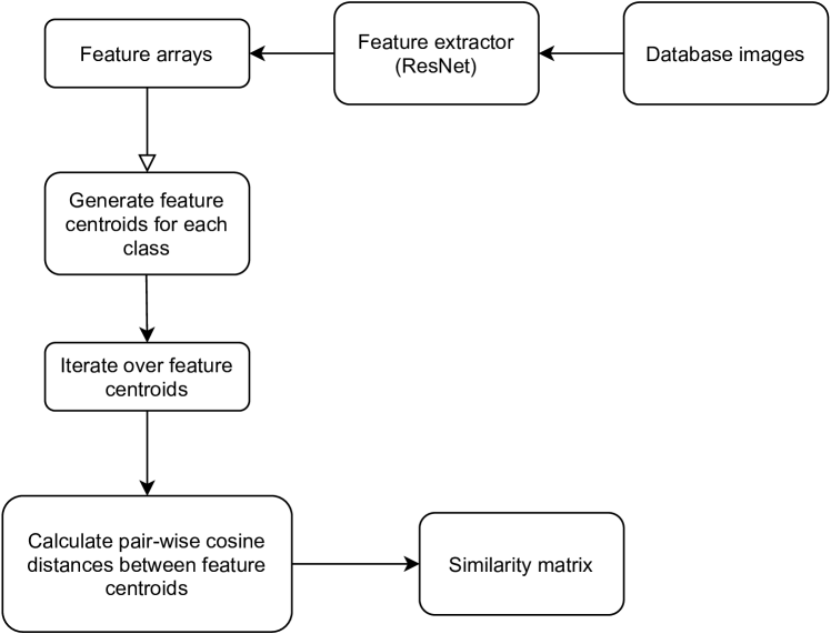
Figure 2: Similarity matrix generation

4.5 Variety contribution ratio

The variety contribution ratio ($v_{r}$) is the second value of the two-part DSI that can help in understanding the data, for a single class, in one go. It considers the overall spread of data compared to the number of samples ($n$) in the class cluster ($c$). We all know that one of the factors overfitting in an image-data algorithm is the variety of the dataset. Basically, the amount of data doesn’t always guarantee a better model, especially if the data samples are redundant. To check whether the data samples are ”actually” contributing to the knowledge of the model or not, I define the variety contribution ratio. The contribution of the data samples is checked by finding the nearest feature $X_{i}$ to each sample and running a distance-based clustering algorithm like DBSCAN ($f_{db}$). The same features extracted earlier $X$ are passed to $f_{db}$. The distance can be set to cosine or any other metric but it has been noticed that the contribution ratio works well if the same distance metric is used for both similarity calculation and the variety contribution ratio, as both of them depend on which layer has been used to extract the feature vectors.

$$v=\rotatebox[origin={c}]{180.0}{E}!(f_{db}(X))$$ (4)

The variety is calculated by the number of unique clusters after passing $X$ to $f_{db}$ with $min{\_}samples$ set to 1. If there is no other feature near(in the similarity distance threshold $z$) then the cluster will remain with a single sample or else it will contain more samples. $z$ can be set according to $S$ or a predefined context but a general value that is seen in most cases sets to about 0.05 (while using cosine distance).

$$v_{r}^{(i)}=\frac{v^{(i)}}{n}=\frac{\rotatebox[origin={c}]{180.0}{E}!(f_{db}(X_{i}))}{n}$$ (5)

If $v_{r}$ is 1, that means all the samples are actually contributing to the knowledge of the model, rather than contributing to overfitting or biasing. If $v_{r}$ is lower, like 0.7, then that means only 70 percent of the data is contributing and the other is not, hence can be comfortably removed to avoid unwanted bias due to data sample redundancy.

The synopsis of the entire methodology can be viewed in Figure 3.

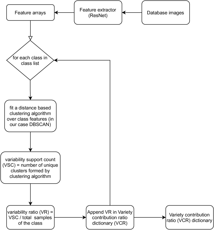
Figure 3: Variety contribution ratio calculation

4.6 Model architectures

I have used 4 traditional vision model architectures to train upon all the datasets. The architectures are: VGG-19, ResNet50, AlexNet and ResNeXt50. All the models are pre-trained on ImageNet and use the standard configuration with Cross entropy loss and step learning rate scheduler.

4.7 Training environment

All the models were trained on Intel Xeon E5-1620 v3 (@ 3.50GHz × 8 CPU) with Nvidia GeForce RTX2080Ti GPU and 16GB of RAM. I used the standard PyTorch library to code and train the model architectures. All models were trained with CUDA enabled.

INPUT: $f{\_}list(n_{c}\times n_{i}\times 2048)$: List of feature arrays of every class image in the database
$class{\_}list$: List of all the classes in the dataset
OUTPUT: $sim{\_}mat(n_{c}\times n_{c})$: Similarity matrix
$n_{i}$: Number of images in that particular class
$n_{c}:$ Number of classes

  Function Similarity_matrix_generator($f{\_}list$, $class{\_}list$):

      $i\leftarrow 0$

     for length of $f{\_}list$ do

        $class{\_}features\leftarrow features[class{\_}list[i]]$

        $model\leftarrow KMeans(n{\_}clusters=1)$

        $model.fit(class{\_}features)$

        $feature{\_}centroids[class{\_}list[i]]\leftarrow model.cluster{\_}centers{\_}$

        $i\leftarrow i+1$

       

      $i\leftarrow 0$

     for length of $feature{\_}centroids$ do

         $j\leftarrow 0$

        for length of $feature{\_}centroids$ do

           $simmat[class{\_}list[i]]\leftarrow cosine(feature{\_}centroids[i],$

                                               $feature{\_}centroids[j])$

           $j\leftarrow j+1$

        $i\leftarrow i+1$

     return $simmat$

Algorithm 1 Algorithm to generate Similarity Matrix

INPUT: $f{\_}list(n_{c}\times n_{i}\times 2048)$: List of feature arrays of every class image in the database
$class{\_}list$: List of all the classes in the dataset
OUTPUT: $variety{\_}contribution{\_}ratio(n_{c}\times 1)$: Variety contribution ratio dictionary
$n_{i}$: Number of images in that particular class
$n_{c}:$ Number of classes

  Function calculate_variability_ratio($f{\_}list,class{\_}list$):

     $variety{\_}contribution{\_}ratio\leftarrow\{\}$

     $i\leftarrow 0$

     for length of $class{\_}list$ do:

        $class{\_}features\leftarrow features[class{\_}list]$

        $X\leftarrow[]$

        for $feature$ in $class{\-}features$:

            $X.append(list(feature))$

        $model\leftarrow DBSCAN(eps=0.05,min{\_}samples=1,$

                                               $metric=`cosine`).fit(X)$

        $variability{\_}supporter{\_}count\leftarrow$ length of $set(model.labels{\_})$

        $variability{\_}ratio\leftarrow variability{\_}supporter{\_}count/$ length of $X$

        $variety{\_}contribution{\_}ratio[class{\_}list[i]]\leftarrow variability{\_}ratio$

         $i\leftarrow i+1$

     return $variety{\_}contribution{\_}ratio$

Algorithm 2 Variety contribution ratio calculation

5 Experiments and Discussions

5.1 Variety contribution ratio usages

1. Extract the maximum out of the current dataset and optimize further.

   The variety contribution ratio helps in reducing the class sample count without disturbing the validation accuracy of the class or the overall model. It means, with this, we can actually make an optimization over the dataset when we need to gain more data or are satisfied with the results of the data. It decreases the computational requirement for people with scarce resources. It also helps in improving the timings for the existing runs and reduces the time when retraining or adding additional visual capabilities.
   

   

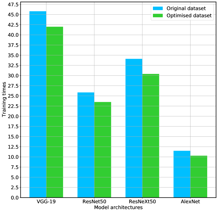
   Figure 4: Comparing training times of each model architecture on original and optimised dataset.

   The variety contribution ratio can help in optimizing the existing dataset and reducing the number of resources required to train with the same knowledge, in turn, making room for more data(varied data) to be appended in the main dataset. Here I train three different model architectures namely, VGG-19, ResNet50, and ResNeXt50 on two versions of the Stanford Dogs dataset and Oxford flowers dataset, original and optimized dataset. The optimized dataset has not been changed in any manner only the number of samples in each class has decreased a little. I set the distance threshold for calculating the variety contribution ratio and remove the samples which are deemed redundant according to the Variety contribution ratio. The results of training on the full dataset and the optimized dataset can be viewed in Figure 5 and 6.
   

   

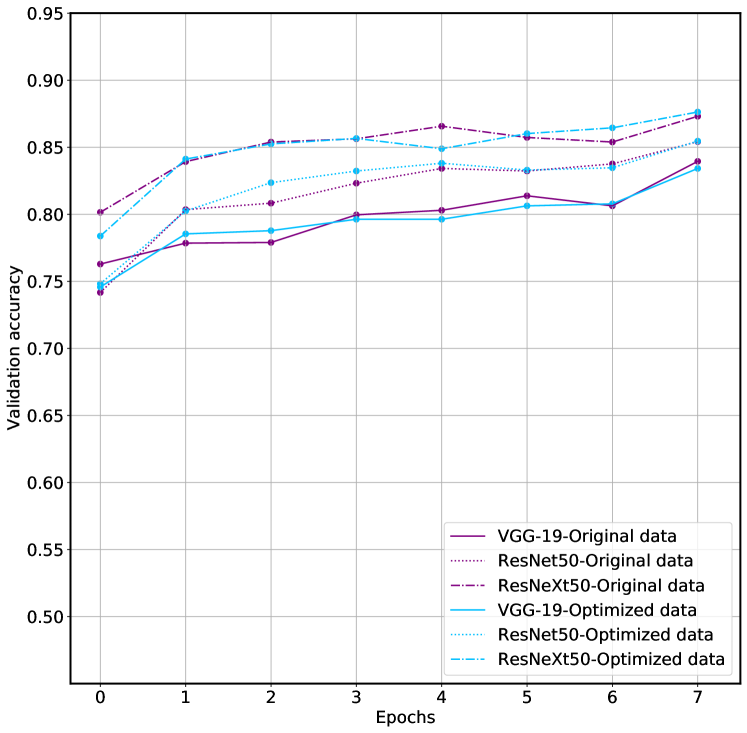
   Figure 5: Validation accuracy on each epoch for Model architectures trained on original and optimized Stanford dogs dataset.

   

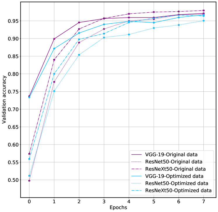
   Figure 6: Validation accuracy on each epoch for Model architectures trained on original and optimized Oxford flowers dataset.

   In Figure 4, we can see that the models trained on the optimized dataset train 10% faster than the ones trained on the original dataset. It shows how the variety contribution ratio can help save time in retraining due to reduced dataset size. Additionally, the model won’t need the same amount of batches to complete an epoch as with the original dataset.

   In Figure 5 and 6, I show the validation accuracies per epoch of all three model architectures trained on two versions of the same dataset. As can be seen, the validation accuracy of all three model architectures is nearly the same, with just a 0.5 percent deviation in the final accuracy. Not just that, but the entire training procedure looks nearly the same. On each epoch, the validation accuracy, as well as the training, can be seen going at the same pace in both the original and optimized version of the dataset. (Refer A and B for all class variety contribution ratio values.)

2. To figure out where the additional data is required.

   With the variety contribution ratio calculated on each class, it is much easier to figure out exactly which class needs further work in terms of getting more data or cleaning. It can help in justifying the class losses and corner one class at a time, and optimize its data. For example, if in a dataset of 5 classes, the class loss for one of the classes is too high, we now check not only the number of samples but also the variety contribution ratio and see if there is enough data according to the data samples used for training as well as testing. If not, more data could be collected to have more varied data samples fit by maintaining the variety contribution ratio after additional sample collection and reduce the overall class loss. With this, the collection of data could be more intuitive and more justifiable.

5.2 Similarity matrix usages

1. Using human-induced conditions to better highly similar classes classification.

   Once we can recognize the classes that the “machine” thinks are too similar, we can induce our human efforts to better the recognition by giving some of the obvious conditions to it. In Figure 7, there are two different species of flowers taken from the Oxford flowers dataset. One of them is a daffodil, and the second is a wildflower. The similarity or the cosine distance between them is 0.03 (which is highly similar). But if we look at them, they have a distinct characteristic (the overall color) that can be appended to the model’s decision which can make the classification between those two classes flawless.

   

   Figure 7: Left: Daffodil and Right: Wildflower

2. Understanding the balance between variety-contribution ratio and similarity matrix.

   In any given dataset, there could be classes that are highly similar as well as highly distinct. The threshold for the variety contribution ratio can be adjusted according to the similarity of the class with other classes in the dataset. For example, if the class of reference is highly similar to other class(es) in the dataset, it is important to increase the variety contribution ratio for the class of reference and one or more classes that share high similarity with that class. As observed in the four-class dataset’s similarity matrix (Table 1), all the classes are highly similar to each other, which can cause a lot of confusion for the model in terms of learning a proper classification between them. Hence, it is not advisable to compress the dataset too much with a very high similarity threshold in the variety contribution ratio calculation. Because with the similarity being this close, we would need samples very particular to that particular class and not discard them off as a redundant sample.

   Table 1: Similarity matrix for four-class custom dataset.

   Class	Bus	Car	Truck	Van
   Bus	0	0.0977	0.0314	0.0468
   Car	0.977	0	0.0685	0.0378
   Truck	0.0314	0.0685	0	0.0292
   Van	0.0468	0.0378	0.0292	0

   Alternatively, if the class is too distinct from other classes in the dataset, the variety contribution ratio need not be that high. Or the overall need for samples itself could be reduced. For example, in a dataset consisting of 5 classes, namely, ball, racket, watch, fish, and tiger, there is no need to indulge in collecting too many data samples or increasing the variety-contribution ratio. The work could easily be completed by less amount of images and normal variety contribution ratio as well.

3. Making a better guess as to which model may better suit the dataset.

   The similarity matrix gives a crucial insight into the overall dataset, in terms of the complexity of the task at hand. If the task is classification or detection, the similarity matrix gives a hint at how difficult that classification could be for a particular model architecture. So, if the overall similarity is too high, shallow models may not work that well with a lower number of computations. Alternatively, if the similarity is too low, realistically speaking, simpler models could also work very well with a significantly lower number of computations.

   For example, in a binary classification, if the similarity between the two classes is too low, there is no need to use neural networks to achieve that task. A simple SVM trained on the features could also do the task easily. Both would need to use CNNs for feature extractions, but SVM could be fitted way faster than a full CNN model. In figure 8, I show two classes from the Oxford flowers dataset, which have high dissimilarity of 0.188. One of the classes is a Pink Primrose, and the other is a Globe Thistle. By training a binary SVM classifier on the features extracted from the earlier method, I achieve 1.0 accuracy on the test set.

   

   Figure 8: Left: Pink Primrose and Right: Globe Thistle

6 Future works and conclusion

As with any new idea, there are a lot of improvements that are possible with DSI’s current methodology and architectures. There are three scenarios in which the work is still going on: First, the variety-contribution ratio’s threshold. Although the threshold could be set by experimenting, there still is the possibility to find out a proper value or mechanism to find the ideal threshold of VC ratio. Second, the way the distances are defined and the possibility of sub-vector comparisons. Right now, the cosine distance used to define the similarity value between two vectors averages the distances of each of the 2048 dimensions of the feature vector. But there could be a mechanism that effectively evaluates the dimensions on which the feature vector is highly similar and the part where it is distinct. This information could also be leveraged to improve the architecture and further understand the machine’s perspective. The last one is the ability to share the entire knowledge in one single value or equation to find a proper balance between the VC ratio and similarity values for each class. This can ease out the model selection techniques as well as dataset usability ranking creations, in turn making it easier for researchers and developers to select models and datasets for a particular task at hand.

I show how the dataset can be effectively evaluated using two of the measurements namely, variety contribution ratio and similarity matrix. The evaluation is shown individually, one for each class. I discussed some of the fundamental scenarios and applications of DSI. And the DSI need not be limited to just visual data. The same work that has been done on visual datasets could be performed on other types of data as well. I invite researchers from various fields to implement their architectures of the DSI on other data types. After a time there is going to be a data crisis and we need to make sure that we extract as much information from as little data as possible. Variety contribution factor is one such road to walk down.

7 Funding Source Declaration

This research did not receive any specific grant from funding agencies in the public, commercial, or not-for-profit sectors.

Appendix A Variety contribution ratio - Stanford Dog Breeds

	Breed	VCR
1	Chihuahua	0.993421
2	Japanese_spaniel	0.848649
3	Maltese_dog	0.976190
4	Pekinese	0.979866
5	Tzu	0.981308
6	Blenheim_spaniel	0.989362
7	papillon	0.923469
8	toy_terrier	0.994186
9	Rhodesian_ridgeback	0.994186
10	Afghan_hound	0.958159
11	basset	0.994286
12	beagle	1.000000
13	bloodhound	0.978610
14	bluetick	0.976608
15	tan_coonhound	0.918239
16	Walker_hound	0.980392
17	English_foxhound	0.923567
18	redbone	0.993243
19	borzoi	0.986755
20	Irish_wolfhound	0.986239
21	Italian_greyhound	0.989011
22	whippet	1.000000
23	Ibizan_hound	0.962766
24	Norwegian_elkhound	0.897959
25	otterhound	0.920530
26	Saluki	0.955000
27	Scottish_deerhound	0.905172
28	Weimaraner	0.981250
29	Staffordshire_bullterrier	0.987097
30	American_Staffordshire_terrier	0.993902
31	Bedlington_terrier	0.846154
32	Border_terrier	0.994186
33	Kerry_blue_terrier	0.770950
34	Irish_terrier	0.982249
35	Norfolk_terrier	0.947674
36	Norwich_terrier	0.967568
37	Yorkshire_terrier	1.000000
38	haired_fox_terrier	0.942675
39	Lakeland_terrier	0.954315
40	Sealyham_terrier	0.742574
41	Airedale	0.995050
42	cairn	1.000000
43	Australian_terrier	0.974490
44	Dandie_Dinmont	0.977778
45	Boston_bull	0.989011
46	miniature_schnauzer	0.993506
47	giant_schnauzer	0.974522
48	standard_schnauzer	0.980645
49	Scotch_terrier	0.987342
50	Tibetan_terrier	0.941748
51	silky_terrier	0.972678
52	coated_wheaten_terrier	0.987179
53	West_Highland_white_terrier	0.988166
54	Lhasa	0.967742
55	coated_retriever	0.980263
56	coated_retriever	0.947020
57	golden_retriever	1.000000
58	Labrador_retriever	0.988304
59	Chesapeake_Bay_retriever	0.994012
60	haired_pointer	0.973684
61	vizsla	0.993506
62	English_setter	0.987578
63	Irish_setter	0.993548
64	Gordon_setter	0.993464
65	Brittany_spaniel	1.000000
66	clumber	0.986667
67	English_springer	0.943396
68	Welsh_springer_spaniel	0.980000
69	cocker_spaniel	0.993711
70	Sussex_spaniel	0.874172
71	Irish_water_spaniel	0.913333
72	kuvasz	0.946667
73	schipperke	0.961039
74	groenendael	0.966667
75	malinois	0.986667
76	briard	0.940789
77	kelpie	1.000000
78	komondor	0.928571
79	Old_English_sheepdog	0.994083
80	Shetland_sheepdog	0.993631
81	collie	0.986928
82	Border_collie	0.993333
83	Bouvier_des_Flandres	0.980000
84	Rottweiler	1.000000
85	German_shepherd	1.000000
86	Doberman	1.000000
87	miniature_pinscher	1.000000
88	Greater_Swiss_Mountain_dog	0.928571
89	Bernese_mountain_dog	0.986239
90	Appenzeller	0.980132
91	EntleBucher	0.955446
92	boxer	1.000000
93	bull_mastiff	0.980769
94	Tibetan_mastiff	0.960526
95	French_bulldog	1.000000
96	Great_Dane	0.987179
97	Saint_Bernard	0.970588
98	Eskimo_dog	0.993333
99	malamute	1.000000
100	Siberian_husky	0.989583
101	affenpinscher	0.953333
102	basenji	0.985646
103	pug	0.995000
104	Leonberg	0.895238
105	Newfoundland	0.994872
106	Great_Pyrenees	0.995305
107	Samoyed	0.899083
108	Pomeranian	0.986301
109	chow	0.989796
110	keeshond	0.911392
111	Brabancon_griffon	0.960784
112	Pembroke	0.988950
113	Cardigan	0.993548
114	toy_poodle	1.000000
115	miniature_poodle	0.993548
116	standard_poodle	0.993711
117	Mexican_hairless	0.851613
118	dingo	0.993590
119	dhole	0.933333
120	African_hunting_dog	0.982249

Appendix B Variety contribution ratio - Oxford Flowers

	Flower species	VCR
1	Pink primrose	1.000000
2	Globe thistle	0.921053
3	Blanket flower	0.885714
4	Trumpet creeper	0.938776
5	Blackberry lily	0.805556
6	Snapdragon	0.852941
7	Colt’s foot	0.753425
8	King protea	0.973684
9	Spear thistle	1.000000
10	Yellow iris	0.973684
11	Globe-flower	0.972222
12	Purple coneflower	0.850000
13	Peruvian lily	0.707692
14	Balloon flower	1.000000
15	Hard-leaved pocket orchid	0.877551
16	Giant white arum lily	1.000000
17	Fire lily	0.941176
18	Pincushion flower	0.914894
19	Fritillary	0.902778
20	Red ginger	1.000000
21	Grape hyacinth	0.941176
22	Corn poppy	0.969697
23	Prince of wales feathers	0.361111
24	Stemless gentian	1.000000
25	Artichoke	0.951613
26	Canterbury bells	0.777778
27	Sweet william	0.590164
28	Carnation	0.937500
29	Garden phlox	0.972222
30	Love in the mist	0.903226
31	Mexican aster	0.821429
32	Alpine sea holly	0.696970
33	Ruby-lipped cattleya	0.919355
34	Cape flower	0.391304
35	Great masterwort	0.840909
36	Siam tulip	0.939394
37	Sweet pea	0.909091
38	Lenten rose	0.944444
39	Barbeton daisy	0.505155
40	Daffodil	0.979592
41	Sword lily	0.960000
42	Poinsettia	0.780822
43	Bolero deep blue	0.969697
44	Wallflower	0.114650
45	Marigold	0.344262
46	Buttercup	0.736842
47	Oxeye daisy	0.578947
48	English marigold	0.740741
49	Common dandelion	0.643836
50	Petunia	0.538835
51	Wild pansy	0.522388
52	Primula	0.800000
53	Sunflower	0.914894
54	Pelargonium	0.375000
55	Bishop of llandaff	0.206522
56	Gaura	0.700000
57	Geranium	0.081395
58	Orange dahlia	0.214286
59	Tiger lily	0.971429
60	Pink-yellow dahlia	0.035294
61	Cautleya spicata	0.305556
62	Japanese anemone	0.645833
63	Black-eyed susan	0.119048
64	Silverbush	0.119048
65	Californian poppy	0.295455
66	Osteospermum	0.039216
67	Spring crocus	1.000000
68	Bearded iris	0.976744
69	Windflower	0.717391
70	Moon orchid	0.939394
71	Tree poppy	0.901961
72	Gazania	0.859375
73	Azalea	0.818182
74	Water lily	0.721088
75	Rose	0.830986
76	Thorn apple	0.863158
77	Morning glory	0.963855
78	Passion flower	0.795122
79	Lotus	0.535714
80	Toad lily	0.823529
81	Bird of paradise	0.971429
82	Anthurium	0.987805
83	Frangipani	0.600000
84	Clematis	0.987805
85	Hibiscus	0.836538
86	Columbine	0.848485
87	Desert-rose	0.833333
88	Tree mallow	0.562500
89	Magnolia	0.901961
90	Cyclamen	0.931034
91	Watercress	0.849673
92	Monkshood	0.829268
93	Canna lily	0.969697
94	Hippeastrum	0.728814
95	Bee balm	0.698113
96	Ball moss	0.970588
97	Foxglove	0.946970
98	Bougainvillea	0.940594
99	Camellia	0.930556
100	Mallow	0.981481
101	Mexican petunia	0.926471
102	Bromelia	0.880000

References

- [1] A. Sharif Razavian, H. Azizpour, J. Sullivan, S. Carlsson, Cnn features off-the-shelf: an astounding baseline for recognition, in: Proceedings of the IEEE conference on computer vision and pattern recognition workshops, 2014, pp. 806–813.
- [2] Y. LeCun, Y. Bengio, et al., Convolutional networks for images, speech, and time series, The handbook of brain theory and neural networks 3361 (10) (1995) 1995.
- [3] H.-C. Shin, H. R. Roth, M. Gao, L. Lu, Z. Xu, I. Nogues, J. Yao, D. Mollura, R. M. Summers, Deep convolutional neural networks for computer-aided detection: Cnn architectures, dataset characteristics and transfer learning, IEEE transactions on medical imaging 35 (5) (2016) 1285–1298.
- [4] N. Jmour, S. Zayen, A. Abdelkrim, Convolutional neural networks for image classification, in: 2018 International Conference on Advanced Systems and Electric Technologies (IC_ASET), IEEE, 2018, pp. 397–402.
- [5] V. N. Gudivada, V. V. Raghavan, Content based image retrieval systems, Computer 28 (9) (1995) 18–22.
- [6] R. Datta, J. Li, J. Z. Wang, Content-based image retrieval: approaches and trends of the new age, in: Proceedings of the 7th ACM SIGMM international workshop on Multimedia information retrieval, 2005, pp. 253–262.
- [7] J. Eakins, M. Graham, Content-based image retrieval.
- [8] J. G. A. Barbedo, Impact of dataset size and variety on the effectiveness of deep learning and transfer learning for plant disease classification, Computers and electronics in agriculture 153 (2018) 46–53.
- [9] A. Krizhevsky, I. Sutskever, G. E. Hinton, Imagenet classification with deep convolutional neural networks, Advances in neural information processing systems 25 (2012) 1097–1105.
- [10] K. Simonyan, A. Zisserman, Very deep convolutional networks for large-scale image recognition, arXiv preprint arXiv:1409.1556.
- [11] C. Szegedy, W. Liu, Y. Jia, P. Sermanet, S. Reed, D. Anguelov, D. Erhan, V. Vanhoucke, A. Rabinovich, Going deeper with convolutions, in: Proceedings of the IEEE conference on computer vision and pattern recognition, 2015, pp. 1–9.
- [12] K. He, X. Zhang, S. Ren, J. Sun, Deep residual learning for image recognition, in: Proceedings of the IEEE conference on computer vision and pattern recognition, 2016, pp. 770–778.
- [13] S. Xie, R. Girshick, P. Dollár, Z. Tu, K. He, Aggregated residual transformations for deep neural networks, in: Proceedings of the IEEE conference on computer vision and pattern recognition, 2017, pp. 1492–1500.
- [14] K. Ding, K. Ma, S. Wang, E. P. Simoncelli, Image quality assessment: Unifying structure and texture similarity, arXiv preprint arXiv:2004.07728.
- [15] C. Ragkhitwetsagul, J. Krinke, B. Marnette, A picture is worth a thousand words: Code clone detection based on image similarity, in: 2018 IEEE 12th International workshop on software clones (IWSC), IEEE, 2018, pp. 44–50.
- [16] B. A. Plummer, M. I. Vasileva, V. Petsiuk, K. Saenko, D. Forsyth, Why do these match? explaining the behavior of image similarity models, in: Computer Vision–ECCV 2020: 16th European Conference, Glasgow, UK, August 23–28, 2020, Proceedings, Part XI 16, Springer, 2020, pp. 652–669.
- [17] L. Wang, D. Rajan, An image similarity descriptor for classification tasks, Journal of Visual Communication and Image Representation 71 (2020) 102847.
- [18] N. A. Shnain, Z. M. Hussain, S. F. Lu, A feature-based structural measure: an image similarity measure for face recognition, Applied Sciences 7 (8) (2017) 786.
- [19] C. Zhang, F. Xie, H. Yu, J. Zhang, L. Zhu, Y. Li, Ppis-join: A novel privacy-preserving image similarity join method, Neural Processing Letters (2021) 1–19.
- [20] A. Khosla, N. Jayadevaprakash, B. Yao, F.-F. Li, Novel dataset for fine-grained image categorization: Stanford dogs, in: Proc. CVPR Workshop on Fine-Grained Visual Categorization (FGVC), Vol. 2, Citeseer, 2011.
- [21] M.-E. Nilsback, A. Zisserman, Automated flower classification over a large number of classes, in: 2008 Sixth Indian Conference on Computer Vision, Graphics & Image Processing, IEEE, 2008, pp. 722–729.
- [22] T.-Y. Lin, M. Maire, S. Belongie, J. Hays, P. Perona, D. Ramanan, P. Dollár, C. L. Zitnick, Microsoft coco: Common objects in context, in: European conference on computer vision, Springer, 2014, pp. 740–755.
- [23] J. Yosinski, J. Clune, Y. Bengio, H. Lipson, How transferable are features in deep neural networks?, arXiv preprint arXiv:1411.1792.
- [24] Huang, Cbir system, https://github.com/pochih/CBIR (2020).
- [25] K. K. Bressem, L. C. Adams, C. Erxleben, B. Hamm, S. M. Niehues, J. L. Vahldiek, Comparing different deep learning architectures for classification of chest radiographs, Scientific reports 10 (1) (2020) 1–16.