Probing triple higgs self coupling and effect of beam polarization in lepton colliders

Abstract

One of the main objectives of almost all future (lepton) colliders is to measure the self-coupling of triple Higgs in the Standard Model. By elongating the Standard Model’s scalar sector, using incipient Higgs doublet along with a quadratic (Higgs) potential should reveal many incipient features of the model and the possibility of the emergence of additional Higgs self-couplings. The self-coupling of the Higgs boson helps in reconstructing the scalar potential. The main objective of this paper is to extract Higgs self-coupling by numerically analyzing several scattering processes governed by two Higgs doublet models (2HDM). These scattering processes include various possible combinations of final states in the triple Higgs sector. The determination of production cross-section of scattering processes is carried out using two different scenarios, with and without polarization of incoming beam and is extended to a center of mass energy up to $\sqrt{s}$ = 3 $TeV$. The computation is carried out in Type-1 2HDM. Here we consider the case of exact alignment limit ($s_{\beta\alpha}$ = 1) and masses of extra Higgs state are equal that is $m_{H}=m_{H^{0}}=m_{A^{0}}=m_{H^{\pm}}$. This choice is made to minimize the oblique parameters. The decays of the final state of each process are investigated to estimate the number of events at integrated luminosity of $1ab^{-1}$ and $3ab^{-1}$.

I Introduction

It is the Higgs mechanism that explains the origin of mass for elementary particles in Standard Model (SM) via an electroweakly broken symmetry mechanism. After the discovery of the most awaited Higgs particle, having a mass of 125 $GeV$, by CMS and ATLAS experiments, one of the major aims of the Large Hadron Collider (LHC) lab1 ; lab2 was to study the properties of this particle such as precision measurement of its mass, production rate, coupling to SM particles, spin-parity, etc. These studies indicate that the discovered particle is in perfect agreement with the SM predictions. The Higgs sector could be more complicated for what is understood as yet and Beyond the Standard Model (BSM) effects could appear from exact measurements of the couplings with fermions and bosons, which can be determined from the Higgs boson production processes and decays. Two Higgs doublet model (2HDM) is one of the simplest extensions of the Standard Model. A second complex doublet SU(2) is added into 2HDM, as a result, we end up having five Higgs states in 2HDM, one CP-odd scalar ($A^{0}$), two CP even scalars ($H^{0}$, $h^{0}$), and two charged Higgs bosons ($H^{+}$, $H^{-}$).
LHC is the biggest particle accelerator, where two beams of protons collide with each other and the resulting collision events are recorded. These events give us information about the beginning of the universe and properties of particles which make up the universe. Hadron colliders are discovery machines as they can reach the highest possible beam energies and therefore, are powerful probes to new energy ranges. For examining the Higgs particles and their properties a lepton collider machine is necessary, as these are the natural precision machines. In lepton collider, the initial states of each event are known accurately and high precision of measurements is possible to achieve. The future circular collider (FCC-ee) lab3 at CERN, the circular electron-positron collider (CEPC) lab4 in china and the international linear collider (ILC) ilc is designed to produce many Higgs bosons and investigate their properties.
The measurement of Higgs self-coupling gives the information about the EWSB mechanism and understanding of the scalar potential of the Higgs field. The process $e^{+}e^{-}\rightarrow ZHH$ which is also known as Higgs-strahlung is best suited to calculate the trilinear Higgs self-coupling in the Standard Model. A similar effort was made earlier where trilinear Higgs couplings with various Higgs bosons pairs connected with the Z boson were examined lab5 . Some of the double and triple Higgs boson couplings were also examined in lab6 ; lab7 . Also trilinear and quartic Higgs coupling have been studied in the past within MSSM lab8 .
In our study, several scattering processes and their possible Higgs self-couplings are determined. The production cross-section as a function of the center of mass-energy and polarization of incoming beam is calculated. The results are obtained within the framework of 2HDM taking into consideration the theoretical and experimental constraints.

II Two Higgs Doublet Model 2HDM

The simplest extension to SM is 2HDM with a different Higgs field but based on an identical gauge field with the same fermion content. The 2HDM consists of 2 Higgs isospin doublets containing hypercharge content of original Higgs field, with 8 degrees of freedom.

$$\phi_{1}=\begin{pmatrix}\phi_{1}^{+}\\ \phi_{1}^{0}\\ \end{pmatrix},\phi_{2}=\begin{pmatrix}\phi_{2}^{+}\\ \phi_{2}^{0}\end{pmatrix}$$

When symmetry is spontaneously broken, in addition to three gauge bosons, the $W^{\pm}$ and $Z^{0}$, we get five new physical Higgs bosons: the two CP-even neutrals h and H, one CP-odd neutral, and two charged scalars $H^{\pm}$.
When a discrete $Z_{2}$ symmetry is applied on the Lagrangian, it results in four possible types of 2HDM which satisfy the GWP lab37 criterion.
In type 1, both quarks and leptons couple to $\phi_{2}$ while in type 2, up type quarks couple to $\phi_{2}$, whereas down type quarks and charged leptons couple to $\phi_{1}$. Similarly, in type 3, up type quarks and charged leptons couple to $\phi_{2}$ while down type quarks couple to $\phi_{1}$. This type is sometimes called flipped. In type 4, all charged leptons couple to $\phi_{1}$ while all quarks couple to $\phi_{2}$. This type is also called lepton specific.

II.1 Softly Broken $Z_{2}$ Symmetry

A discrete $Z_{2}$ symmetry is applied on the Lagrangian which constrain it. The Higgs basis is defined as

$$\phi_{1}=\begin{pmatrix}G^{+}\\ \frac{1}{\sqrt{2}}[\nu+S_{1}+\iota G^{0}]\\ \end{pmatrix},\phi_{2}=\begin{pmatrix}H^{+}\\ \frac{1}{\sqrt{2}}[S_{2}+\iota S_{3}]\end{pmatrix}$$

where $\quad(\iota=1,2)$ and $\nu=\sqrt{\nu^{2}_{1}+\nu^{2}_{2}}$. The hermitian Klein-Gordon fields are $G^{0}$, $S_{1}$, $S_{2}$ and $S_{3}$ while complex Klein-Gordon fields are $G^{+}$ and $H^{+}$.
Invoking a $Z_{2}$ symmetry removes flavor changing neutrals current (FCNCs). Therefore in the Higgs basis, the scalar potential is written as

$$V(\phi_{1},\phi_{2})=m^{2}_{1}|\phi_{1}|^{2}+m^{2}_{2}|\phi_{2}|^{2}-[m^{2}_{3}\phi_{1}^{+}\phi_{2}+h.c.]+\frac{\Lambda_{1}}{2}\Bigg{|}(\phi_{1}^{+}\phi_{1})^{2}+\frac{\Lambda_{2}}{2}(\phi_{2}^{+}\phi_{2})^{2}+\Lambda_{3}|\phi_{1}|^{2}|\phi_{2}|^{2}+\Lambda_{4}|\phi_{1}^{+}\phi_{2}|\Bigg{|}^{2}$$ (1)

$$+\Bigg{[}\frac{\Lambda_{5}}{2}(\phi_{1}^{+}\phi_{1})^{2}+h.c.\Bigg{]}+[(\Lambda_{6}\phi_{1}^{+}\phi_{1}+\Lambda_{7}\phi_{2}^{+}\phi_{2})\phi_{1}^{+}\phi_{2}+h.c.],$$ (2)

The coupling constant $m^{2}_{1}$, $m^{2}_{2}$, $\Lambda_{1}$, $\Lambda_{2}$, $\Lambda_{3}$ and $\Lambda_{4}$ are real and the complex parameters are $m^{2}_{3}$, $\Lambda_{5}$, $\Lambda_{6}$ and $\Lambda_{7}$ but for simplification they are taken as real. The scalar potential can be decomposed as a sum of quadratic, cubic and quartic interactions. The quadratic terms define the physical Higgs state and its masses. Diagonalization of the quadratic mass terms gives masses of all extra Higgs bosons lab38 . The $\sin{(\beta-\alpha)}$ is the mixing angle among the CP-even Higgs state and is also denoted by $s_{\beta\alpha}$.

The exact alignment limit i.e. $s_{\beta\alpha}$ = 1 is considered, so that $h^{0}$ become indistinguishable from the Standard Model Higgs boson with respect to coupling and mass. Hence there are only six independent parameters of the model which are important for our study, which include $m_{h}$, $m_{H^{0}}$, $m_{A^{0}}$, the ratio of vacuum expectation value $\tan{\beta}$, $s_{\beta\alpha}$ and ${m_{3}}^{2}$. The parameter ${m_{3}}^{2}$ indicates that, how is the discrete symmetry broken lab39 . In Equation  2 the cubic and quartic terms define the interactions and couplings between the new states in 2HDM.

II.2 Theoretical And Experimental Constraints

The parameters of scalar potential in 2HDM are reduced both by the theoretical developments, as well as results of experimental searches. The theoretical constraints to which 2HDM is subjected, comprise of vacuum stability, unitarity, and perturbativity.

• Stability: Requirement of a stable vacuum keeps the potential bounded from below. The potential must be positive at large values of fields for any direction in the plane lab40 ; lab41 .

• Unitarity: Unitarity constraints do not allow the scattering amplitudes to have probability more than unity. The amplitude needs to be flat at asymptotically large values of energy lab42 ; lab43 .

• Perturbitivity: The potential needs to be perturbative to fulfill the requirement that all quartic couplings of scalar potential obey $\Lambda_{i}\leq 8\pi$ for all $i$

With the help of 2HDMC-1.7.0 lab44 , the parameters are tested as if, they obey the above mentioned constraints. The 2HDM parameters are also constrained by experimental researches. According to a recent study lab45 , it is observed that flavor limits are present and Figure 3 in there shows the available region which is not excluded even today. The charged Higgs $H^{\pm}$ present in 2HDM, which is comparable to SM, also makes a novel contribution in flavor limits. According to current experimental results at LHC (give reference) and (give reference), masses of all extra Higgs bosons are set to be equal that is $m_{H}=m_{H^{0}}m_{A^{0}}=m_{H^{\pm}}$. This choice minimizes the oblique parameters and all the electroweak observables are close to SM. The decay of $H^{0}$ to vector boson pair is suppressed in the exact alignment limit. According to lab43 in type-1, the neutral meson mixing and results of $B^{0}_{s}\rightarrow\mu^{+}\mu^{-}$ restrict the low $\tan{\beta}$. The analysis is therefore, carried out in range 2 $<\tan{\beta}<$ 40. The regions in which theoretical constraints are obeyed by ${m_{3}}^{2}$ are measured with the help of 2HDMC.

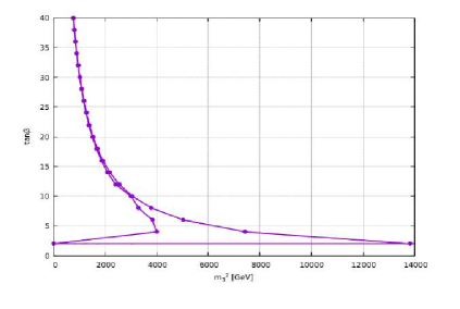
Figure 1: The plot between soft symmetry breaking term versus $\tan{\beta}$. The region under bounded curves shows the theoretical constraints obeyed.

Benchmark	Yukawa Type	$m_{h}$ $[GeV]$	$m_{H}=m_{A}=m_{H}^{+}$ [GeV]	$s_{\beta\alpha}$	$t_{\beta}$
1	Type-I	125	175	1	2.40

Table 1: The range of independent parameters calculated within Type-1 2HDM

II.3 Higgs Self-couplings in 2HDM

In 2HDM, Higgs self-couplings as a function of $\Lambda_{i}$ are given by Equations  3 to  8. The values for two independent parameters are selected to be $s_{\beta\alpha}$ = 1 and $c_{\beta\alpha}$ = 0. Due to exact alignment limit and equal masses of all extra Higgs bosons, three other parameters $\Lambda_{4}$, $\Lambda_{5}$ and $\Lambda_{6}$ also vanish. Among all the Higgs self couplings, only the one given by $g_{hhH}$ vanishes. However the couplings $g_{hHH}$ and $g_{hAA}$ are equal to each other and $g_{HHH}/g_{HAA}$ = 3. These predictions can also be checked experimentally. If $\Lambda_{345}=\Lambda_{3}+\Lambda_{4}+\Lambda_{5}$, then we can write

$$g_{h^{0}h^{0}h^{0}}=-3\iota\nu((\Lambda_{7}c^{2}_{\beta\alpha}+3\Lambda_{6}s^{2}_{\beta\alpha})c_{\beta\alpha}+(\Lambda_{345}c^{2}_{\beta\alpha}+\Lambda_{1}\delta^{2}_{\beta\alpha})s_{\beta\alpha})\underset{c\beta\alpha\rightarrow 0}{=}-3\iota\nu\Lambda_{1}$$ (3)

$$g_{h^{0}h^{0}H^{0}}=-\iota\nu((\Lambda_{345}(1-3s^{2}_{\beta\alpha})+3\Lambda_{1}s^{2}_{\beta\alpha})c_{\beta\alpha}+3(\Lambda_{6}(2-3s^{2}_{\beta\alpha})-\Lambda_{7}c^{2}_{\beta\alpha})s_{\beta\alpha})\underset{c\beta\alpha\rightarrow 0}{=}0$$ (4)

$$g_{h^{0}H^{0}H^{0}}=-\iota\nu((3\Lambda_{1}c^{2}_{\beta\alpha}+\Lambda_{345}(3s^{2}_{\beta\alpha}-2))s_{\beta\alpha}+3(\Lambda_{6}+\Lambda_{7}\%s^{2}_{\beta\alpha}-3\Lambda_{6}s^{2}_{\beta\alpha})c_{\beta\alpha})\underset{c\beta\alpha\rightarrow 0}{=}-\iota\nu\Lambda_{3}$$ (5)

$$g_{h^{0}A^{0}A^{0}}=-\iota\nu(\Lambda_{7}c_{\beta\alpha}+(\Lambda_{3}+\Lambda_{4}-\Lambda_{5})s_{\beta\alpha})\underset{c\beta\alpha\rightarrow 0}{=}-\iota\nu\Lambda_{3}$$ (6)

$$g_{H^{0}H^{0}H^{0}}=-3\iota\nu((\Lambda_{1}c^{2}_{\beta\alpha}+\Lambda_{345}s^{2}_{\beta\alpha})c_{\beta\alpha}-\Lambda_{7}s^{2}_{\beta\alpha}-3\Lambda_{6}c^{2}_{\beta\alpha})s_{\beta\alpha}\underset{c\beta\alpha\rightarrow 0}{=}3\iota\nu\Lambda_{7}$$ (7)

$$g_{H^{0}A^{0}A^{0}}=-\iota\nu((\Lambda_{3}+\Lambda_{4}-\Lambda_{5})c_{\beta\alpha}-\Lambda_{7}s_{\beta\alpha})\underset{c\beta\alpha\rightarrow 0}{=}\iota\nu\Lambda_{7}$$ (8)

III Tripple Higgs Self Coupling and Production Cross-section

It is normally believed that ILC will perform efficiently in precision measurements as compared to LHC, due to it’s clean environment, fixed center-of-mass energy, and attainability of polarised beam. This fact emphasizes the importance of ILC for Higgs sector in terms of calculations of different scattering processes, their self-couplings, branching ratios and estimation of number of events.

III.0.1 Measurement of Higgs Self-Coupling

The trilinear self-coupling can be measured directly or indirectly by using the Higgs-boson-pair production cross section, or through the measurement of single-Higgs-boson production and decay modes, respectively. In fact, the Higgs-decay partial widths and the cross sections of the main single-Higgs production processes depend on the Higgs-boson self-coupling via weak loops, at next-to-leading order in electroweak interaction. Let’s consider the scattering process $e^{-}e^{+}\rightarrow Zhh$ to study the trilinear coupling of the Higgs boson. In SM the Feynman diagrams of this process are shown in Figure  2.

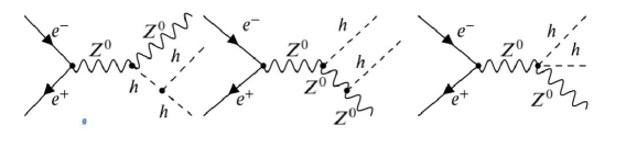
Figure 2: The left-most diagram contains the Higgs self coupling vertex corresponding to the process $e^{+}e^{-}\rightarrow Zhh$.

The measurement of Higgs self-coupling within 2HDM is difficult due to the presences of more than one Higgs. The couplings in which $h^{0}$, $H^{0}$, and $A^{0}$ are intermediated, do not make a noticeable contribution because of their absolute value, which is less than $10^{-6}$, so they can be neglected. Significant contributions are found to be from $Z^{0}$ coupling only, that’s why only those Feynman diagrams are taken into account in which Z boson is intermediated. The scattering processes with various combinations of trilinear Higgs self-couplings need to be considered, i.e. $ZHh$, $ZAh$, $HHH$, $hhh$, $Ahh$, $AAh$, $AAH$, $Hhh$ and $Hhh$.

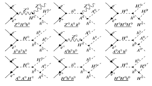
Figure 3: The feynman diagram of various processes in 2HDM. Their amplitude shows that their cross-section is less than $10^{-11}$ pb, so their self coupling could be neglected.

The Feynman diagrams of the possible processes are shown in Figure  3. Their cross-section is less than $10^{-11}$pb, therefore it is not possible to detect them and can be easily neglected.

Scatering Processes	Higgs self-coupling
$e^{-}e^{+}\rightarrow Z^{0}A^{0}A^{0}$	$g_{h^{0}A^{0}A^{0}}$
$e^{-}e^{+}\rightarrow Z^{0}H^{0}H^{0}$	$g_{h^{0}H^{0}H^{0}}$
$e^{-}e^{+}\rightarrow Z^{0}h^{0}h^{0}$	$g_{h^{0}h^{0}h^{0}}$
$e^{-}e^{+}\rightarrow A^{0}H^{0}h^{0}$	$g_{H^{0}A^{0}A^{0}}$
$e^{-}e^{+}\rightarrow A^{0}H^{0}H^{0}$	$g_{H^{0}A^{0}A^{0}}$, $g_{H^{0}H^{0}H^{0}}$

Table 2: The tripple Higgs self-coupling contributing to scattering process while using the exact alignment limit equal to one and extra Higgs masses to be equal.

To calculate the Higgs self-coupling in two Higgs doublet model, we consider the second set of scattering processes shown in Table  2. These scattering processes are the only ones which can give the cross-section greater than attobarn. In Equation  LABEL:eq:4.4b $g_{h^{0}h^{0}H^{0}}$ approaches zero so this coupling vanishes. The cross-section of scattering process $e^{-}e^{+}\rightarrow ZAA$ makes it possible to determine the coupling $g_{h^{0}A^{0}A^{0}}$. The coupling $g_{h^{0}H^{0}H^{0}}$ can be determined by measuring the cross-section of process $e^{-}e^{+}\rightarrow ZHH$. The cross-section of $e^{-}e^{+}\rightarrow Zhh$ extracts the coupling $g_{h^{0}h^{0}h^{0}}$ which could be the same as determined in SM. The coupling $g_{H^{0}A^{0}A^{0}}$ can be determined by two processes, $e^{-}e^{+}\rightarrow AHh$ and $e^{-}e^{+}\rightarrow AHH$, whereas the last mentioned process can also give $g_{H^{0}H^{0}H^{0}}$.

IV The production cross-section of scattering processes

For the computation of production cross-section of various scattering processes, CalcHEP$\_$3.7.6 package lab46 is used. The parameters of Standard Model are used from the lab47 , which are $m_{e}$ = 0.51099 $MeV$, $m_{Z}$ = 91.1876 $GeV$ and $s_{w}$ = 0.474. The Higgs boson mass is taken to be $m_{h}$ = 125.09 $GeV$. The 2HDM parameters are already discussed in previous chapter. The cross-sections of various scattering process are given below:

IV.0.1 $e^{-}e^{+}\rightarrow Zhh$

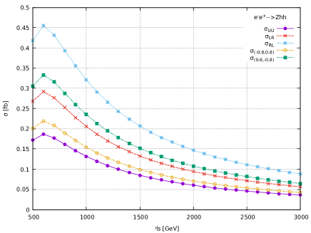
Figure 4: Total cross-section $\sigma$ (fb) as a function of $\sqrt{s}$ (GeV) at Higgs masses $m_{H}$ = 150 $GeV$ or $m_{H}$ = 175 $GeV$, $\tan{\beta}$ = 10 and $s_{\beta\alpha}$=1 are shown.

The cross-section of this prominent channel is shown in the Figure  4. It can be seen that the maximum cross-section of the unpolarized beam is approximately 0.187 $fb$ at 0.6 $TeV$, and decreases for higher energies. However the polarized beam enhances the cross-section as compared to the unpolarized beam. The right-handed electron beam and left-handed positron beam ($\sigma_{RL}$) maximize the cross-section which is around 0.455 $fb$ at 0.6 $TeV$. Moreover, the distribution of left-handed electron beam and right-handed positron beam ($\sigma_{LR}$), and two cases of polarization beam $\sigma_{(0.6,-0.8)}$ and $\sigma_{(-0.6,0.8)}$ are also given in Table  3.

	0.6 TeV	1 TeV	3 TeV
	$m_{\phi}$=150=175=300=500	$m_{\phi}$=150=175=300=500	$m_{\phi}$=150=175=300=500
$\sigma_{UU}$	0.187 $\pm$ 0.02	0.132 $\pm$ 0.0204	0.036 $\pm$ 0.01
$\sigma_{LR}$	0.292 $\pm$ 0.031	0.206 $\pm$ 0.031	0.056 $\pm$ 0.02
$\sigma_{RL}$	0.455 $\pm$ 0.049	0.321 $\pm$ 0.050	0.082 $\pm$ 0.034
$\sigma_{(0.6,-0.8)}$	0.332 $\pm$ 0.036	0.235 $\pm$ 0.036	0.065 $\pm$ 0.027
$\sigma_{(-0.6,0.8)}$	0.219 $\pm$ 0.023	0.155 $\pm$ 0.02	0.045 $\pm$ 0.018

Table 3: The cross-section in $fb$ with unpolarized and polarized incoming $e^{-}e^{+}$ beams. Where masses of extra Higgs states are varied over a range of $m_{H}$ = 150 $GeV$ to $m_{H}$ = 500 $GeV$. In all cases, distribution of cross-section for both scenarios of with and without polarized beams is the same.

0.6 TeV

1 TeV

3 TeV

$m_{\phi}$ =150

$m_{\phi}$ =175

$m_{\phi}$ =300

$m_{\phi}$ =500

$m_{\phi}$ =150

$m_{\phi}$ =175

$m_{\phi}$ =300

$m_{\phi}$ =500

$m_{\phi}$ =150

$m_{\phi}$ =175

$m_{\phi}$ =300

$m_{\phi}$ =500

$e^{-}e^{+}\rightarrow AHh$

$\sigma_{UU}$

0.0059 $\pm$ 0.0012

0.0023 $\pm$ 0.0004

0.0 $\pm$ 0.0

0.0 $\pm$ 0.0

0.0078 $\pm$ 0.0023

0.0059 $\pm$ 0.0016

0.0011 $\pm$ 0.0002

0.0 $\pm$ 0.0

0.0012 $\pm$ 0.0015

0.0010 $\pm$ 0.0014

0.0005 $\pm$ 0.0004

0.0002 $\pm$ 0.0001

$\sigma_{LR}$

0.0091 $\pm$ 0.0019

0.0037 $\pm$ 0.0007

0.0 $\pm$ 0.0

0.0 $\pm$ 0.0

0.0121 $\pm$ 0.0035

0.0093 $\pm$ 0.0025

0.00168 $\pm$ 0.0035

0.0 $\pm$ 0.0

0.0018 $\pm$ 0.0023

0.0016 $\pm$ 0.0018

0.00092 $\pm$ 0.00059

0.0004 $\pm$ 0.0002

$\sigma_{RL}$

0.0143 $\pm$ 0.0029

0.0057 $\pm$ 0.0012

0.0 $\pm$0.0

0.0 $\pm$0.0

0.0189 $\pm$0.0056

0.0145 $\pm$ 0.0038

0.0026 $\pm$ 0.0006

0.0 $\pm$ 0.0

0.0029 $\pm$ 0.0038

0.0025 $\pm$ 0.0028

0.0014 $\pm$ 0.0009

0.00069 $\pm$ 0.0003

$\sigma_{(0.6,-0.8)}$

0.0105 $\pm$ 0.0022

0.0042 $\pm$ 0.0008

0.0 $\pm$ 0.0

0.0 $\pm$ 0.0

0.0138 $\pm$ 0.0040

0.0186 $\pm$ 0.0049

0.0019 $\pm$ 0.0004

0.0 $\pm$ 0.0

0.0021 $\pm$ 0.0027

0.0018 $\pm$ 0.0021

0.0010 $\pm$ 0.0007

0.0005 $\pm$ 0.0002

$\sigma_{(-0.6,0.8)}$

0.0069 $\pm$ 0.0014

0.0027 $\pm$ 0.0006

0.0 $\pm$ 0.0

0.0 $\pm$ 0.0

0.0091 $\pm$ 0.0026

0.0070 $\pm$ 0.0018

0.0012 $\pm$ 0.0002

0.0 $\pm$ 0.0

0.0014 $\pm$ 0.0018

0.0012 $\pm$ 0.0014

0.0007 $\pm$ 0.0004

0.0003 $\pm$ 0.0001

$e^{-}e^{+}\rightarrow AHH$

$\sigma_{UU}$

0.0018 $\pm$ 0.0004

0.0002 $\pm$ 0.00004

0.0 $\pm$ 0.0

0.0 $\pm$ 0.0

0.0042 $\pm$ 0.0013

0.0023 $\pm$ 0.0006

0.000014 $\pm$ 0.000003

0.0 $\pm$ 0.0

0.0009 $\pm$ 0.0011

0.0006 $\pm$ 0.0006

0.00017 $\pm$ 0.00087

0.000033 $\pm$ 0.0000094

$\sigma_{LR}$

0.0029 $\pm$ 0.0006

0.00033 $\pm$ 0.00006

0.0 $\pm$ 0.0

0.0 $\pm$ 0.0

0.0065 $\pm$ 0.002

0.0035 $\pm$ 0.0009

0.00002152 $\pm$ 0.0000043

0.0 $\pm$ 0.0

0.0014 $\pm$ 0.0017

0.0010 $\pm$ 0.0009

0.00027 $\pm$ 0.00013

0.000051 $\pm$ 0.000017

$\sigma_{RL}$

0.0046 $\pm$ 0.0010

0.00052 $\pm$ 0.0001

0.0 $\pm$ 0.0

0.0 $\pm$ 0.0

0.010 $\pm$ 0.003

0.0055 $\pm$ 0.0015

0.000033 $\pm$ 0.0000068

0.0 $\pm$ 0.0

0.0022 $\pm$ 0.002

0.0016 $\pm$ 0.0015

0.0004 $\pm$ 0.00020

0.000082 $\pm$ 0.000023

$\sigma_{(0.6,-0.8)}$

0.0038 $\pm$ 0.0008

0.0003 $\pm$ 0.0008

0.0 $\pm$ 0.0

0.0 $\pm$ 0.0

0.0074 $\pm$ 0.0023

0.0040 $\pm$ 0.001

0.000024 $\pm$ 0.0000049

0.0 $\pm$ 0.0

0.0016 $\pm$ 0.0019

0.0011 $\pm$ 0.001

0.00031 $\pm$ 0.00015

0.0000602 $\pm$ 0.000017

$\sigma_{(-0.6,0.8)}$

0.0022 $\pm$ 0.0004

0.00025 $\pm$ 0.00005

0.0 $\pm$ 0.0

0.0 $\pm$ 0.0

0.0049 $\pm$ 0.0015

0.0026 $\pm$ 0.0007

0.000016 $\pm$ 0.0000033

0.0 $\pm$ 0.0

0.0010 $\pm$ 0.0012

0.00075 $\pm$ 0.0007

0.00020 $\pm$ 0.0001

0.000039 $\pm$ 0.0000112

$e^{-}e^{+}\rightarrow ZHH/ZAA$

$\sigma_{UU}$

0.0527 $\pm$ 0.0060

0.0278 $\pm$ 0.0030

0.0 $\pm$ 0.0

0.0 $\pm$ 0.0

0.075 $\pm$ 0.011

0.062 $\pm$ 0.009

0.0152 $\pm$ 0.00200

0.0 $\pm$ 0.0

0.031 $\pm$ 0.009

0.030 $\pm$ 0.008

0.02423 $\pm$ 0.0052

0.0158 $\pm$ 0.0029

$\sigma_{LR}$

0.0824 $\pm$ 0.0093

0.0436 $\pm$ 0.0049

0.0 $\pm$ 0.0

0.0 $\pm$ 0.0

0.117 $\pm$ 0.017

0.097 $\pm$ 0.04

0.0237 $\pm$ 0.0031

0.0 $\pm$ 0.0

0.049 $\pm$ 0.015

0.047 $\pm$ 0.013

0.0379 $\pm$ 0.0082

0.0247 $\pm$ 0.0045

$\sigma_{RL}$

0.1284 $\pm$ 0.0146

0.0679 $\pm$ 0.0075

0.0 $\pm$ 0.0

0.0 $\pm$ 0.0

0.183 $\pm$ 0.027

0.151 $\pm$ 0.022

0.0370 $\pm$ 0.0048

0.0 $\pm$ 0.0

0.077 $\pm$ 0.023

0.073 $\pm$ 0.019

0.0590 $\pm$ 0.0127

0.0386 $\pm$ 0.0071

$\sigma_{(0.6,-0.8)}$

0.0941 $\pm$ 0.0106

0.0498 $\pm$ 0.0054

0.0 $\pm$ 0.0

0.0 $\pm$ 0.0

0.134 $\pm$ 0.019

0.110 $\pm$ 0.011

0.0271 $\pm$ 0.0035

0.0 $\pm$ 0.0

0.056 $\pm$ 0.016

0.054 $\pm$ 0.014

0.0432 $\pm$ 0.0094

0.0287 $\pm$ 0.0052

$\sigma_{(-0.6,0.8)}$

0.0618 $\pm$ 0.0071

0.0327 $\pm$ 0.0089

0.0 $\pm$ 0.0

0.0 $\pm$ 0.0

0.088 $\pm$ 0.013

0.072 $\pm$ 0.010

0.0178 $\pm$ 0.0023

0.0 $\pm$ 0.0

0.037 $\pm$ 0.011

0.035 $\pm$ 0.0095

0.0284 $\pm$ 0.0061

0.0185 $\pm$ 0.0034

Table 4: The cross-section in $fb$ with unpolarized and polarized incoming $e^{-}e^{+}$ beams. Where masses of extra Higgs states are varied over a range of $m_{H}$ = 150 $GeV$ to $m_{H}$ = 500 $GeV$. In all cases, distribution of cross-section for both scenarios of with and without polarized beams is the same.

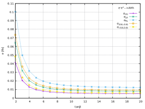
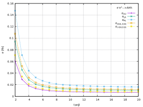
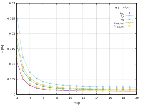
Figure 5: Figure shows dependency of tan$\beta$ on $\sigma(pp\rightarrow AHh)$ at (a) $\sqrt{s}$=0.6 TeV, (b) $\sqrt{s}$=1 TeV and (c) $\sqrt{s}$=3 TeV energies.

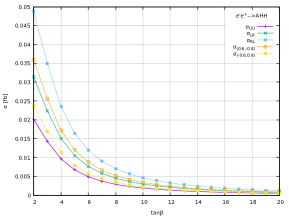
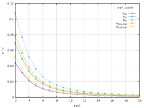
Figure 6: In Figures the production cross sections $\sigma(pp\rightarrow AHH)$ are shown as a function of tan$\beta$ at (a) 0.6 TeV, (b) 1 TeV and (c) 3 TeV energies.

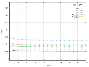
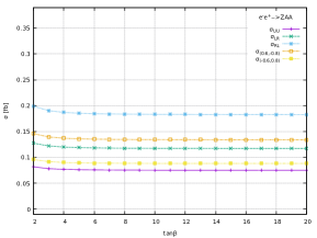
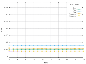
Figure 7: Figure (a) is plotted to discuss the bechaviour of $\sigma(pp\rightarrow ZAA)$ at $\sqrt{s}$=0.6 TeV, in whereas (b) and (c) are plotted same variables at $\sqrt{s}$=1 TeV and $\sqrt{s}$=3 TeV respectively

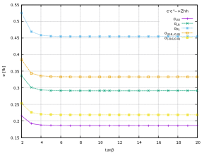
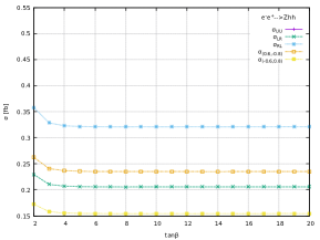
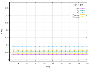
Figure 8: Figure shows dependency of tan$\beta$ on $\sigma(pp\rightarrow Zhh)$ at (a) $\sqrt{s}$=0.6 TeV, (b) $\sqrt{s}$=1 TeV and (c) $\sqrt{s}$=3 TeV energies.

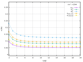
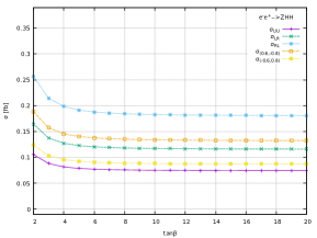
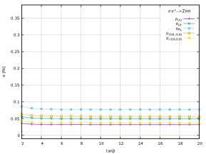
Figure 9: In Figures the production cross sections $\sigma(pp\rightarrow ZHH)$ are shown as a function of tan$\beta$ at (a) 0.6 TeV, (b) 1 TeV and (c) 3 TeV energies.

	0.6 TeV				1 TeV				3 TeV
	$\tan{\beta}$=5	$\tan{\beta}$=10	$\tan{\beta}$=15	$\tan{\beta}$=20	$\tan{\beta}$=5	$\tan{\beta}$=10	$\tan{\beta}$=15	$\tan{\beta}$=20	$\tan{\beta}$=5	$\tan{\beta}$=10	$\tan{\beta}$=15	$\tan{\beta}$=20
	$e^{-}e^{+}\rightarrow Zhh$
$\sigma_{UU}$	0.1869	0.1863	0.1864	0.186	0.1319	0.1316	0.1317	0.1317	0.036253	0.0361733	0.03616	0.0362
$\sigma_{LR}$	029203	0.29120	0.29126	0.29130	0.20615	0.20572	0.20573	0.20573	0.056621	0.056543	0.056539	0.056557
$\sigma_{RL}$	0.45565	0.45426	0.45435	0.45442	0.31259	0.32089	0.32096	0.32098	0.088306	0.088241	0.088241	0.088193
$\sigma_{(0.6,-0.8)}$	0.33387	0.33297	0.33301	0.33299	0.23570	0.23521	0.23530	0.23525	0.064696	0.064651	0.064676	0.064674
$\sigma_{(-0.6,0.8)}$	0.21934	0.21877	0.21878	0.21880	0.15479	0.15452	0.15454	0.15455	0.042510	0.042491	0.042457	0.042514
	$e^{-}e^{+}\rightarrow AHh$
$\sigma_{UU}$	0.017277	0.01045	0.00093411	0.0089632	0.013257	0.0077706	0.0068967	0.0065998	0.0021479	0.001047	0.001047	0.00099589
$\sigma_{LR}$	0.015155	0.0091414	0.0081716	0.0078409	0.020702	0.01214	0.010770	0.010317	0.0033532	0.0018687	0.0016357	0.0015611
$\sigma_{RL}$	0.023581	0.014264	0.012748	0.012232	0.032320	0.018947	0.016800	0.016090	0.0052484	0.0029070	0.0025522	0.0024360
$\sigma_{(0.6,-0.8)}$	0.017277	0.010454	0.0093411	0.0089632	0.023686	0.013889	0.012320	0.011787	0.0038544	0.0021296	0.0018715	0.0017796
$\sigma_{(-0.6,0.8)}$	0.011354	0.0068721	0.0061365	0.0058895	0.015560	0.0091174	0.0080898	0.0077460	0.0025196	0.0014044	0.0012263	0.0011680
	$e^{-}e^{+}\rightarrow AHH$
$\sigma_{UU}$	0.0067367	0.001894	0.0008613	0.00048807	0.014793	0.0064978	0.0018905	0.001071	0.00321	0.00090088	0.00041045	0.00023214
$\sigma_{LR}$	0.010523	0.0029595	0.0013454	0.00076264	0.023111	0.0064978	0.0029554	0.0016753	0.0050175	0.0014085	0.00063930	0.00036364
$\sigma_{RL}$	0.016417	0.0046182	0.0020992	0.001897	0.036058	0.010142	0.0046089	0.0026143	0.0078280	0.0022009	0.0010019	0.00056732
$\sigma_{(0.6,-0.8)}$	0.012032	0.0033842	0.0015387	0.00087216	0.026419	0.0074374	0.0033764	0.0019149	0.0057319	0.0016118	0.00073268	0.00041471
$\sigma_{(-0.6,0.8)}$	0.0079058	0.0022240	0.0010107	0.00057310	0.017364	0.0048834	0.0022192	0.0012581	0.0037654	0.0010560	0.00048088	0.00027258
	$e^{-}e^{+}\rightarrow ZHH$
$\sigma_{UU}$	0.058131	0.052392	0.051358	0.050993	0.078495	0.074928	0.07438	0.07412	0.031811	0.03148	0.031411	0.031407
$\sigma_{LR}$	0.090831	0.0818630	0.080237	0.079662	0.12264	0.11703	0.11611	0.11579	0.049703	0.049168	0.049067	0.049034
$\sigma_{RL}$	0.14170	0.12771	0.12517	0.1247	0.19129	0.18261	0.18117	0.18065	0.077557	0.076655	0.076611	0.076518
$\sigma_{(0.6,-0.8)}$	0.10384	0.093580	0.091721	0.091077	0.14022	0.13385	0.13275	0.13237	0.056871	0.056211	0.056085	0.056052
$\sigma_{(-0.6,0.8)}$	0.068235	0.061480	0.060274	0.059846	0.092134	0.087936	0.087239	0.086994	0.037366	0.036951	0.036839	0.036841
	$e^{-}e^{+}\rightarrow ZAA$
$\sigma_{UU}$	0.054229	0.05272	0.052419	0.052313	0.075971	0.075097	0.074993	0.074924	0.031578	0.031489	0.031469	0.031467
$\sigma_{LR}$	0.084719	0.08235	0.081905	0.081737	0.11868	0.11735	0.11712	0.11702	0.049323	0.049201	0.049158	0.049131
$\sigma_{RL}$	0.13219	0.12851	0.12777	0.12751	0.18521	0.18306	0.18277	0.18261	0.076973	0.076717	0.76681	0.076691
$\sigma_{(0.6,-0.8)}$	0.096858	0.094178	0.093642	0.093460	0.13569	0.13418	0.13389	0.13384	0.056379	0.056242	0.056228	0.056194
$\sigma_{(-0.6,0.8)}$	0.063644	0.061869	0.061510	0.061416	0.089156	0.088173	0.087995	0.087925	0.037060	0.036940	0.036912	0.036923

Table 5: A complete scan of most relevant parameters of 5 different production processes at Higgs mass $m_{\phi}$ =150 GeV is performed

IV.0.2 $e^{-}e^{+}\rightarrow ZHH/ZAA$

Consider the scattering process $e^{-}e^{+}\rightarrow ZHH/ZAA$ for determination of cross-section distribution. Since according to Equations  LABEL:eq:4.5b and  LABEL:eq:4.6b, the couplings $g_{h^{0}A^{0}A^{0}}$ and $g_{h^{0}H^{0}H^{0}}$ of both scattering processes are same, and in terms of parameter space, $m_{H}$ and $m_{A}$ are also identical, hence these two scattering process $e^{-}e^{+}\rightarrow ZHH$ and $e^{-}e^{+}\rightarrow ZAA$ can be considered same. Therefore, the cross-section as a function of center of mass of energy for both, becomes equal. The plots for different polarizations of beam are shown in Figure  10. The scattering amplitudes for Feynman diagrams shown in Figure  11 and  12 are same. We consider two different fixed values of extra Higgs states i.e., $m_{H}$ = 175 $GeV$ and $m_{H}$ = 150 $GeV$ and compare their cross-section. From Figure  10, it is clear that for $m_{H}$ = 175 $GeV$ the maximum cross-section of unpolarized beam is 0.062 $fb$ at 1 $TeV$ which decreases slowly with increase in energy. The maximum cross-section of right handed polarized electron and left handed polarized positron beam is around 0.151 $fb$. When $m_{H}$ =150 $GeV$, then the unpolarized cross-section reaches about 0.075 $fb$ and then decreases slowly with higher energy. Additionally $\sigma_{RL}$ = 0.183 $fb$, which shows that $RL$ scenario enhances the cross-section. From comparison of two mass values, it is clear that a value of 150 $GeV$ shows maximum cross-section as compared to 175 $GeV$.

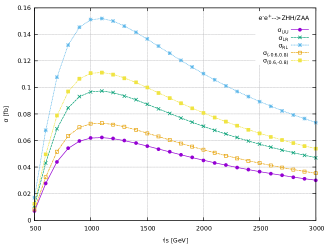
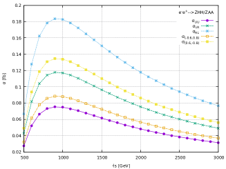
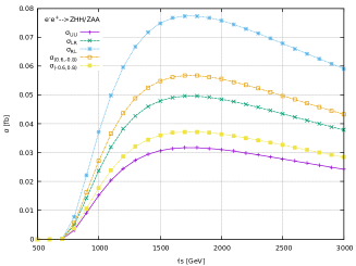
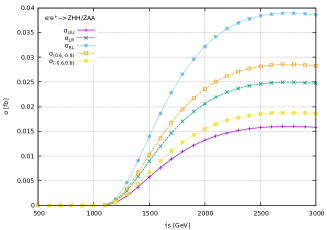
Figure 10: Total cross-section $\sigma$ ($fb$) as a function of $\sqrt{s}$ ($GeV$) at 2HDM. Higgs mass value $m_{H}$ = 175 $GeV$, $\tan{\beta}$ = 10 and $s_{\beta\alpha}$ = 1 are used (left). The Higgs masses $m_{H}$ = 150 $GeV$, $\tan{\beta}$ = 10 and $s_{\beta\alpha}$ = 1 are used (right)

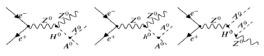
Figure 11: Feynman diagrams contributing to the scattering process $e^{-}e^{+}\rightarrow\text{ZAA}$.

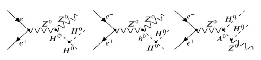
Figure 12: Feynman diagrams contributing to the scattering process $e^{-}e^{+}\rightarrow\text{ZHH}$ at ILC.

IV.0.3 $e^{-}e^{+}\rightarrow AHh$

For the next scattering process $e^{-}e^{+}\rightarrow AHh$, the distributions are shown in Figure  13. When the mass of extra Higgs states are taken as 175 $GeV$ then the cross-section of $\sigma_{UU}$ (unpolarized) = 0.0059 $fb$ at $\sqrt{s}$=1 TeV. The maximum cross-section of polarized beam is $\sigma_{RL}$ = 0.0145 $fb$. Similarly when $m_{H}$ = $m_{A}$ = $m_{H^{\pm}}$ =150 $GeV$ are used then unpolarized cross-section is 0.0078 $fb$ and right-handed polarized electron beam and left-handed polarized positron beam ($\sigma_{RL}$) is 0.0189 $fb$. Coupling $g_{H^{0}A^{0}A^{0}}$ can be extracted from this scattering process but the cross-section is quite small.

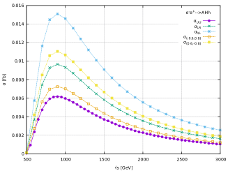
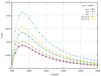
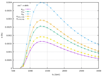
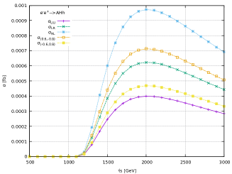
Figure 13: The distribution of cross-section $\sigma$ ($fb$) as a function of $\sqrt{s}$ ($GeV$) in 2HDM. The Higgs masses $m_{H}$ = $m_{A}$ = $m_{H^{\pm}}$ =175 $GeV$, $\tan\beta$=10 and $s_{\beta\alpha}$ = 1 are used (left). The Higgs masses are taken to be $m_{H}$ = $m_{A}$ = $m_{H^{\pm}}$ = 150 $GeV$, $\tan\beta$=10 and $s_{\beta\alpha}$ = 1 (right).

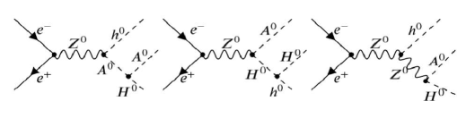
Figure 14: Feynman diagrams contributing to the scattering process $e^{-}e^{+}\rightarrow\text{ZHH}$ at ILC.

IV.0.4 $e^{-}e^{+}\rightarrow AHH$

The last cross-section is calculated for the scattering process $e^{-}e^{+}\rightarrow AHH$. The cross-section plot is shown in Figure  15. This process has smallest cross-section as compared to others. The unpolarized beam has a cross-section of 0.0023 $fb$ at $\sqrt{s}$ = 1$TeV$, where $m_{H}$ = $m_{A}$ = $m_{H^{\pm}}$ = 175 $GeV$. In case of $m_{H}$ = $m_{A}$ = $m_{H^{\pm}}$ = 150 $GeV$ the cross-section of unpolarized beam is around 0.0042 $fb$ at 1$TeV$ which drops rapidly with increase in energy.

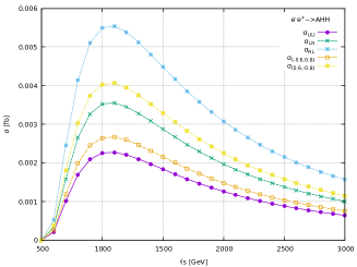
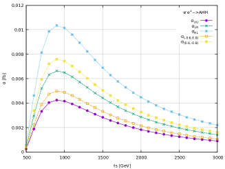
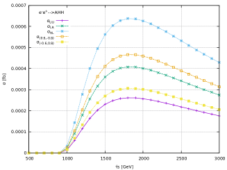
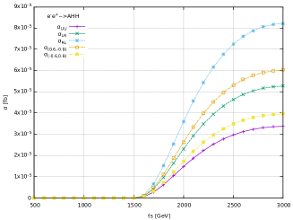
Figure 15: The distribution of cross-section $\sigma$ ($fb$) as a function of $\sqrt{s}$ ($GeV$) at 2HDM. The Higgs masses $m_{H}$ = $m_{A}$ = $m_{H^{\pm}}$ = 175 $GeV$, $\tan{\beta}$ = 10 and $s_{\beta\alpha}$=1 are used (left). The Higgs masses are taken as $m_{H}$ = $m_{A}$ = $m_{H^{\pm}}$ = 150 $GeV$, $\tan{\beta}$ = 10 and $s_{\beta\alpha}$=1 (right).

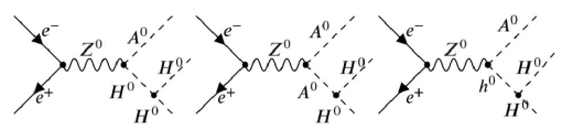
Figure 16: The feynman diagram for scattering process $e^{-}e^{+}\rightarrow$ AHH at ILC.

V Dependance of $\tan{\beta}$ and $m_{H}$ On The Production Cross-section

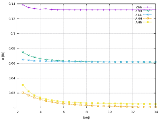
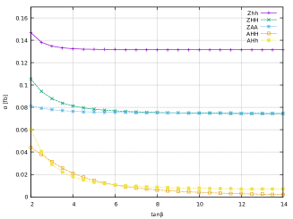
Figure 17: Cross-section distribution as a function of $\tan\beta$ for all the processes at $\sqrt{s}$ = 1 $TeV$. The values used are, $m_{H}$= 175 $GeV$ (left) and $m_{H}$ = 150 $GeV$ (right).

The variation of production cross-section for all processes, with change in $\tan{\beta}$ at $\sqrt{s}$ = 1$TeV$ is shown in Figure 5.11. It can be seen that for the process Zhh, production cross-section remains constant for the two mass values. The reason being the fact that, the coupling $g_{h^{0}h^{0}h^{0}}$ for this process is the same as SM one. In the exact alignment limit, the production cross-section for processes ZHH and ZAA have the same distribution because both processes are a function of the same factors as given in Equations  LABEL:eq:4.5b and  LABEL:eq:4.6b. Next, the production cross-section of the processes AHH and AHh are maximum at the low value of $\tan{\beta}$ and decreases at higher values of $\tan{\beta}$.

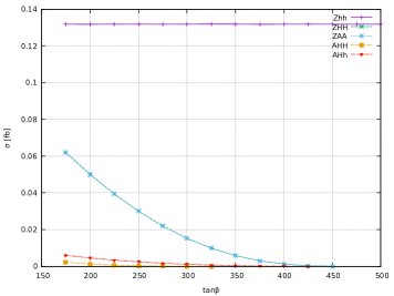
Figure 18: The distribution of cross-section as a function of tan$\beta$ at $\sqrt{s}$ = 1 $TeV$, where $s_{\beta\alpha}$ = 1 and $m_{\phi}$ = 150 GeV.

The distribution of cross-section as a function of $m_{H}$ is shown in Figure  18. It can be seen that the cross-section for all processes, decreases with increasing values of $m_{H}$. This is as expected because, when the mass of all the extra Higgs states is increased the phase space becomes narrow for particles in the final state. The process $Zhh$ is an exception, for which the production cross-section remains constant and does not change with a change in the value of $m_{H}$.

VI Identifying the Processes

In this section, possible decays of neutral Higgs boson are discussed, and possible colliders for analyzing each of the processes are perceived. The expected number of events and some possible background channels are also discussed.

VI.1 Decays Of Neutral Higgs Bosons

The branching ratios and decay widths for neutral Higgs Bosons a are calculated using 2HDMC-1.7.0, whose parameters are explained in Table  LABEL:table:9a. The branching ratios for Higgs particles $H^{0}$, $h^{0}$ and $A^{0}$ are given as a pie chart. Decay width is defined as the probability of occurance of a specific decay process within a given amount of time. The calculation involves determination of the decay width of neutral Higgs boson based on masses of particles involved and their relevant vertices. While the branching ratio of each Higgs boson remains stable. Further the decay channels for each of the Higgs bosons remain the same whereas the Higgs mass $m_{H}$ is changed.

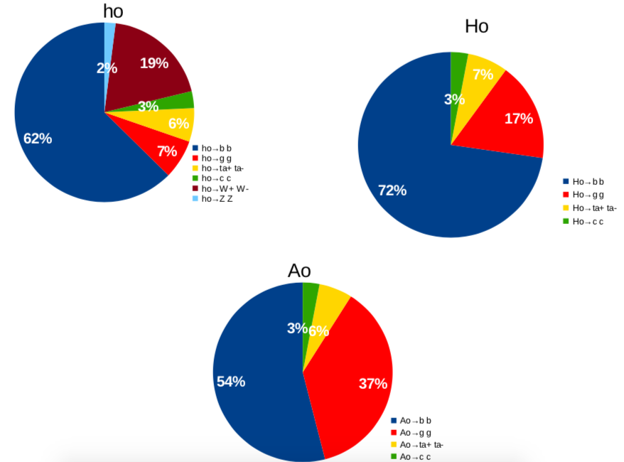
Figure 19: The branching ratios of all neutral Higgs boson decays for parameters defined in Table  LABEL:table:9a.

From Figure  19, it is clear that the prominent decay channel for all the neutral Higgs bosons is through b-quarks pair. The branching ratio for $h^{0}\rightarrow b\bar{b}$ is $62\%$. Similarly the branching ratios for $H^{0}\rightarrow b\bar{b}$ and $A^{0}\rightarrow b\bar{b}$ are $72\%$ and $54\%$ respectively. The other possible decay channels for $h^{0}$, $H^{0}$, and $A^{0}$ are g g and c c pairs. It is logical to say that, due to b-quark, gluon, and c-quark pairs the prominent pattern for each neutral Higgs boson is the di-jet final state in the detector. The next common decay channel is the $\tau\tau$. But the branching ratio of this process is small as compared to the di-jet signal. The $h^{0}$ also has other decay channels, which is through $W^{+}W^{-}$ and $ZZ$ pair. Hence these decay channels can be considered as favorable but problem can arise due to leptonic decays of $W$-boson and extra $Z$-boson in the final state. Therefore the hadronic decay channels of $h^{0}$ boson promise more in the extraction of its pattern.

VI.2 Identification of processes and background channels

In the previous section, decay channels of neutral Higgs boson are discussed and so acquiring the detector pattern of each channel is quite easy. The $Z$ boson decays through a hadronic, leptonic, and invisible channel. The branching ratios of $Z$ boson are $Z\rightarrow q\bar{q}$ ($\sim$0.70), $Z\rightarrow l\bar{l}$ ($\sim$0.10) and invisible($\sim$0.20), respectively. Hence there will be 4 $b$-quark jets +2 light jets (coming from $Z$ boson decay) in the final states. Unfortunately, the branching ratio of leptonic decay is small in comparison to the hadronic branching ratio, and there could be fewer events collected in the detector. Some possible patterns at the detectors, percentage of events and expected number of events are given in Tables  6 and  7 for an integrated luminosity values of $1ab^{-1}$ and $3ab^{-1}$.

Detector patern	$Z^{0}A^{0}A^{0}$	$Z^{0}H^{0}H^{0}$	$Z^{0}h^{0}h^{0}$	$Z^{0}H^{0}h^{0}$	$Z^{0}H^{0}H^{0}$
4b-quarks jets+2jets	20.41	36.28	26.91	28.31	35.76
6 jets	60	58	37.30	62	78.71

Table 6: The percentage of events for different decay channels.

Detector patern	$Z^{0}A^{0}A^{0}$		$Z^{0}H^{0}H^{0}$		$Z^{0}h^{0}h^{0}$		$Z^{0}H^{0}h^{0}$		$Z^{0}H^{0}H^{0}$
	$1ab^{-1}$	$3ab^{-1}$	$1ab^{-1}$	$3ab^{-1}$	$1ab^{-1}$	$3ab^{-1}$	$1ab^{-1}$	$3ab^{-1}$	$1ab^{-1}$	$3ab^{-1}$
4b-quarks jets+2jets	12	39	22	66	35	105	2	4	0.8	2.4
6 jets	38	114	37	111	48	144	3	9	1.7	5.1

Table 7: Expected number of events for integrated luminosity of $1ab^{-1}$ and $3ab^{-1}$.

It is assumed that International Linear Collider can achieve a total integrated luminosity of $1ab^{-1}$ and $3ab^{-1}$ in its lifetime. The number of events that are expected for various processes in that case are given in Table  7at $\sqrt{s}$ = 1 $TeV$. Where the $m_{H}$ =175 $GeV$ and $\tan{\beta}$ = 10 are used. Unfortunately, some events for scattering process $A^{0}H^{0}h^{0}$ and $A^{0}H^{0}H^{0}$ are $\leq$10 and $\leq$ 6 with $3ab^{-1}$. The number of events could be increased by using polarized incoming beams. However, only this may not give enough cross-section to be useful for the measurement of these two processes. There is some background signal which can hide the actual processes. In SM the most relevant and expected background channels are $e^{+}e^{-}\rightarrow Zb\bar{b}b\bar{b}$, $e^{+}e^{-}\rightarrow Zcccc$ and $e^{+}e^{-}\rightarrow ZZ\rightarrow b\bar{b}b\bar{b}$. Hence reconstruction of the Higgs mass in each event could be beneficial. If neutral Higgses do not decay through bb pairs, then such b-quarks pair will give an invariant mass value that lies outside of the Higgs mass range and such events can be excluded. If the efficiency of b-tagging is measured around $80\%$ or higher, and we require $H_{i}H_{j}\rightarrow b\bar{b}b\bar{b}$ + hadronic decay, this offers a definite pattern at the detector which is 4 b-tagged jets +2 light jets. A notable amount of events can be obtained from this pattern, whereas a big fraction of the background signal could be eliminated, because of b-tagged jet requirements. A Monte Carlo simulation of each of the processes is required to evaluate trigger efficiency and acceptance of the detector for different decay channels.

VII Conclusion

In this study, the production cross-section of various scattering processes is calculated in $e^{+}e^{-}$ collider. The scattering process selected to determine the triple Higgs-self coupling is governed by 2HDM. The 2HDM is examined by considering experimental constraints on charged Higgs boson. These constraints probe the exact alignment limit $s_{\beta\alpha}$ = 1. There are eight possible Higgs self-couplings, two out of which, the ones for charged Higgs, are not discussed in this study. Due to exact alignment limit $s_{\beta\alpha}$ = 1, one of the Higgs self-coupling $g_{h^{0}h^{0}H^{0}}$ vanishes, therefore only five Higgs self-coupling survive out of eight. The contribution of Higgs self-coupling for each scattering process is described in Table 5.1. The coupling could be determined using the process $Z^{0}h^{0}h^{0}$ which is the same as in Standard Model. The final state of the process $Z^{0}A^{0}A^{0}$ and $Z^{0}H^{0}H^{0}$ helps in extraction of coupling $g_{h^{0}A^{0}A^{0}}$ and $g_{h^{0}H^{0}H^{0}}$. These processes have an acceptable cross-section. Similarly the coupling $g_{H^{0}A^{0}A^{0}}$ is obtained by the process $e^{+}e^{-}\rightarrow A^{0}h^{0}h^{0}$. But the cross-section is in atto-barn, and might not be enough for accumulation of sufficient number of events. At last, the process $e^{+}e^{-}\rightarrow A^{0}H^{0}H^{0}$ extracts the Higgs self-coupling $g_{H^{0}H^{0}H^{0}}$ with the help of $g_{H^{0}A^{0}A^{0}}$, but only if it could ever possibly be determined through the process $A^{0}H^{0}H^{0}$. Although, examining the previous process could be difficult, calculating the coupling $g_{H^{0}H^{0}H^{0}}$ is also a challenge using $A^{0}H^{0}H^{0}$ process. The calculation of production cross-section for all the above scattering processes, both with and without polarized beams shows that the incoming polarized beam enhance the cross-section. The right-handed electron beam and left-handed positron beam enhanced the cross-section up to a factor of 2.4 for all processes. The calculation is carried out in exact alignment limit $s_{\beta\alpha}$ = 1 and $m_{H}$ = 175 $GeV$ and $m_{H}$ = 150 $GeV$. The calculation shows that the cross-section increases when $m_{H}$ =150 $GeV$ is used in comparison to 175 $GeV$, for all processes, except $Z^{0}h^{0}h^{0}$. The decay widths (not given) and branching ratios of neutral Higgs bosons are also calculated. The study shows that all neutral Higgs bosons have identical decay channels for the specific choice of parameters. The dominant decay channel of all neutral Higgs bosons is through $b\bar{b}$ pair, gluon pair, $c\bar{c}$ pair and with a small fraction of $\tau\bar{\tau}$. For the measurement of cross-section distribution, ILC has the biggest potential for contribution as compared to the proposed all other future lepton colliders. ILC will operate at a centre of mass energy ranging up to 1TeV. The Future Circular Collider can also make measurements and compete for the couplings $g_{h^{0}h^{0}h^{0}}$, $g_{h^{0}A^{0}A^{0}}$ and $g_{h^{0}H^{0}H^{0}}$ by operating at a centre of mass energy range up to 0.5 $TeV$. However, the Circular Electron-Positron Collider does have sufficient centre of mass energy to investigate the Higgs self-coupling even for a process like ZHH in SM. The invention of the Higgs boson at LHC has established the Higgs mechanism, generating mass to all particles. This was the last piece of SM and further no clue to new physics has been observed. The simplest extension of SM is 2HDM. This study shows the possible measurement of trilinear Higgs-coupling in the future lepton colliders, which plays a vital role in reconstructing Higgs potential.

References

- (1) Aad, G., Abajyan, T., Abbott, B., Abdallah, J., Khalek, S. A., Abdelalim, A. A., … Bansil, H. S. (2012). Observation of a new particle in the search for the Standard Model Higgs boson with the ATLAS detector at the LHC. Physics Letters B, 716(1), 1-29.
- (2) Chatrchyan, S., Khachatryan, V., Sirunyan, A. M., Tumasyan, A., Adam, W., Aguilo, E., … Junior, W. A. (2012). Observation of a new boson at a mass of 125 GeV with the CMS experiment at the LHC. Physics Letters B, 716(1), 30-61
- (3) Bicer, M., Yildiz, H. D., Yildiz, I., Coignet, G., Delmastro, M., Alexopoulos, T., … & TLEP Design Study Working Group. (2014). First look at the physics case of TLEP. Journal of High Energy Physics, 2014(1), 164.
- (4) Xiao, M., Gao, J., Wang, D., Su, F., Wang, Y. W., Bai, S., & Bian, T. J. (2016). Study of CEPC performance with different collision energies and geometric layouts. Chinese Physics C, 40(8), 087001.
- (5) A.Djouadi et al. International Linear Collider Reference Design Report Volume 2: Physics at the ILC, arXiv:0709.1893 [hep-ph]
- (6) Arhrib, A., Benbrik, R., & Chiang, C. W. (2008). Probing triple Higgs couplings of the two Higgs doublet model at a linear collider. Physical Review D, 77(11), 115013.
- (7) Ferrera, G., Guasch, J., Lopez-Val, D., & Sola, J. (2008). Triple Higgs boson production in the linear collider. Physics Letters B, 659(1-2), 297-307.
- (8) Dubinin, M. N., & Semenov, A. V. (2003). Triple and quartic interactions of Higgs bosons in the two-Higgs-doublet model with CP-violation. The European Physical Journal C-Particles and Fields, 28(2), 223-236.
- (9) Chalons, G., Djouadi, A., & Quevillon, J. (2018). The neutral Higgs self-couplings in the (h) MSSM. Physics Letters B, 780, 74-80.
- (10) Halzen, F., Martin, A. D., & Mitra, N. (1985). Quarks and leptons: An introductory course in modern particle physics. American Journal of Physics, 53, 287-287..
- (11) Gribbin, J. (2000). Q is for quantum: An encyclopedia of particle physics. Simon and Schuster.
- (12) Christman, J. The Weak Interaction. Physnet. Michigan State University, 2001.
- (13) De Rujula, A., Gavela, M. B., & Hernandez, P. (1999). Neutrino oscillation physics with a neutrino factory. Nuclear Physics B, 547(1-2), 21-38.
- (14) Bernstein, J. (1974). Spontaneous symmetry breaking, gauge theories, the Higgs mechanism and all that. Reviews of modern physics, 46(1), 7.
- (15) Higgs, P. W. (1964). Broken symmetries and the masses of gauge bosons. Physical Review Letters, 13(16), 508-509.
- (16) Higgs, P. W. (1964). Broken symmetries, massless particles and gauge fields. Phys. Lett., 12, 132-133.
- (17) Ta-Pei Cheng and Ling-Fong Li, ”Guage theory of elementary particle physics”, Oxford University Press, 1984.
- (18) M. E. Peskin and D. V. Schroeder, ”An introduction to Quantum Field Theory”, Westview Press, 1995.
- (19) J. Einasto, ”Dark Matter”, arXiv:0901.0632 [astro-ph.CO]P. L. Biermann and F. Munyaneza, ”The nature of dark matter”, arXiv:astro-ph/0702164.
- (20) J. N. Bahcall et al., ”Solar Neutrinos: The First Thirty Years”, Westview, Boul-der, CO (2002).
- (21) Sakharov, A. D. (1998). Violation of CP-invariance, C-asymmetry, and baryon asymmetry of the Universe. In In The Intermissions Collected Works on Research into the Essentials of Theoretical Physics in Russian Federal Nuclear Center, Arzamas-16 (pp. 84-87).
- (22) Berger, C., Genzel, H., Grigull, R., Lackas, W., Raupach, F., Klovning, A., … & PLUTO Collaboration. (1979). Evidence for gluon bremsstrahlung in e+ e? annihilations at high energies. Physics Letters B, 86(3-4), 418-425.
- (23) Barber, D. P., Becker, U., Benda, H., Boehm, A., Branson, J. G., Bron, J., … & Zhu, R. Y. (1979). Discovery of three-jet events and a test of quantum chromodynamics at petra. Physical Review Letters, 43(12), 830
- (24) Electroweak, T. S., Groups, H. F., ALEPH Collaboration, DELPHI Collaboration, L3 Collaboration, OPAL Collaboration, … & LEP Electroweak Working Group. (2006). Precision electroweak measurements on the Z resonance. Physics Reports, 427(5-6), 257-454.
- (25) Evans, L. (2007). The large hadron collider. New Journal of Physics, 9(9), 335.
- (26) Fujii, K., Grojean, C., Peskin, M. E., Barklow, T., Gao, Y., Kanemura, S., … & Yamamoto, H. (2015). Physics case for the international linear collider. arXiv preprint arXiv:1506.05992.
- (27) Holzer, B. J. (2017). Introduction to particle accelerators and their limitations. arXiv preprint arXiv:1705.09601.1
- (28) Adolphsen, C. (2013). The International Linear Collider Technical Design Report-Volume 3. I: Accelerator& in the Technical Design Phase No. arXiv: 1306.6353.
- (29) Adolphsen, C., Barone, M., & Barish, B. (2013). The international linear collider. Technical design report. Vol. 3.2. Accelerator baseline design (No. DESY–13-062-VOL. 3.2). Deutsches Elektronen-Synchrotron (DESY).
- (30) Han, T. (2006). Collider phenomenology: Basic knowledge and techniques. In Physics In D 4 Tasi 2004: TASI 2004 (pp. 407-454).
- (31) Behnke, T., Brau, J. E., Foster, B., Fuster, J., Harrison, M., Paterson, J. M., … & Yamamoto, H. (2013). The international linear collider technical design report-volume 1: Executive summary. arXiv preprint arXiv:1306.6327.
- (32) Dannheim, D., Lebrun, P., Linssen, L., Schulte, D., Simon, F., Stapnes, S., … & Wells, J. (2012). CLIC e+ e-linear collider studies. arXiv preprint arXiv:1208.1402.
- (33) Boland, M. J., Felzmann, U., Giansiracusa, P. J., Lucas, T. G., Rassool, R. P., Balazs, C., … & Vainola, J. (2016). Updated baseline for a staged Compact Linear Collider. CERN Publishing.
- (34) Linssen, L., Miyamoto, A., Stanitzki, M., & Weerts, H. (2012). Physics and detectors at CLIC: CLIC conceptual design report. arXiv preprint arXiv:1202.5940.
- (35) Diaz, R. A., & Martinez, R. (2003). The custodial symmetry. arXiv preprint hep-ph/0302058.
- (36) Gunion, J. F. (2002). Extended higgs sectors. arXiv preprint hep-ph/0212150.
- (37) Lee, T. D. (1973). A theory of spontaneous T violation. Physical Review D, 8(4), 1226.
- (38) Honorez, L. L., Nezri, E., Oliver, J. F., & Tytgat, M. H. (2007). The inert doublet model: an archetype for dark matter. Journal of Cosmology and Astroparticle Physics, 2007(02), 028.Glashow,
- (39) Glashow, S. L., & Weinberg, S. (1977). Natural conservation laws for neutral currents. Physical Review D, 15(7), 1958.
- (40) Kanemura, S., & Yagyu, K. (2015). Unitarity bound in the most general two Higgs doublet model. Physics Letters B, 751, 289-296.
- (41) Gunion, J. F., & Haber, H. E. (2003). CP-conserving two-Higgs-doublet model: the approach to the decoupling limit. Physical Review D, 67(7), 075019.
- (42) El Kaffas, A. W., Khater, W., Ogreid, O. M., & Osland, P. (2007). Consistency of the two-Higgs-doublet model and CP violation in top production at the LHC. Nuclear Physics B, 775(1-2), 45-77.
- (43) Deshpande, N. G., & Ma, E. (1978). Pattern of symmetry breaking with two Higgs doublets. Physical Review D, 18(7), 2574.
- (44) Ginzburg, I. F., & Ivanov, I. P. (2005). Tree-level unitarity constraints in the most general two Higgs doublet model. Physical Review D, 72(11), 115010.
- (45) Eriksson, D., Rathsman, J., & Stal, O. (2010). 2HDMC-two-Higgs-doublet model calculator. Computer Physics Communications, 181(1), 189-205.
- (46) Enomoto, T., & Watanabe, R. (2016). Flavor constraints on the Two Higgs Doublet Models of Z 2 symmetric and aligned types. Journal of High Energy Physics, 2016(5), 2.
- (47) Belyaev, A., Christensen, N. D., & Pukhov, A. (2013). CalcHEP 3.4 for collider physics within and beyond the Standard Model. Computer Physics Communications, 184(7), 1729-1769.
- (48) Eidelman, S., Hayes, K. G., Olive, K. E., Aguilar-Benitez, M., Amsler, C., Asner, D., … & Webber, B. R. (2004). Review of particle physics. Physics letters B, 592(1-4), 1-5.