Optical Flow Estimation for Spiking Camera

Abstract

As a bio-inspired sensor with high temporal resolution, the spiking camera has an enormous potential in real applications, especially for motion estimation in high-speed scenes. However, frame-based and event-based methods are not well suited to spike streams from the spiking camera due to the different data modalities. To this end, we present, SCFlow, a tailored deep learning pipeline to estimate optical flow in high-speed scenes from spike streams. Importantly, a novel input representation is introduced which can adaptively remove the motion blur in spike streams according to the prior motion. Further, for training SCFlow, we synthesize two sets of optical flow data for the spiking camera, SPIkingly Flying Things and Photo-realistic High-speed Motion, denoted as SPIFT and PHM respectively, corresponding to random high-speed and well-designed scenes. Experimental results show that the SCFlow can predict optical flow from spike streams in different high-speed scenes. Moreover, SCFlow shows promising generalization on real spike streams. All codes and constructed datasets will be released after publication.

1 Introduction

Optical flow estimation has always been a popular topic in computer vision and played important roles in a wide range of applications, such as object segmentation [2018OpticalFlowForSegmentation], video enhancement [wang2020deep], and action recognition [tu2019action]. However, the breakthrough of this field in high-speed scenes is impeded by blurry images from traditional cameras with low frame rate.

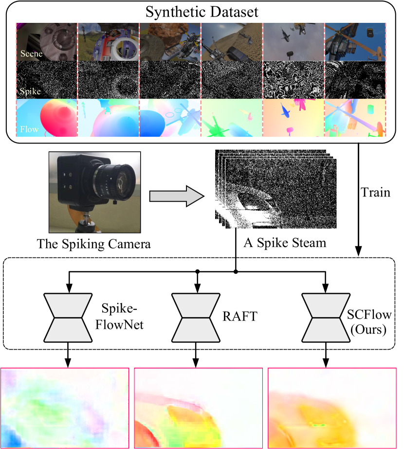
Figure 1: The optical flow estimation for a real spike stream which records a car traveling at a speed of 100 km/h. We compare our SCFlow to event-based method (Spike-FlowNet [lee2020spike]) and frame-based method (RAFT [teed2020raft]). All methods use spike streams as input and are trained on proposed synthetic dataset (SPIFT). Results show that our proposed method has better performance which clearly distinguishes regions with different motion and accurately predict optical flow in each region.

The emergence of neuromorphic cameras [dvs1, dvs2, dvs3, dvs4, dvs5, spikecode, spikecamera] provides a new perspective for optical flow estimation in high-speed scenes. Some works [zhu2018multivehicle, zhu2019unsupervised, lee2020spike] raise the interest in event cameras [dvs1, dvs2, dvs3, dvs4, dvs5] and show optical flow in high-speed scene can be directly estimated from an event stream. However, the event stream that only encodes the change of luminance intensity might be insufficient for optical flow estimation in all regions of a scene, especially for regions with weak or no textures. Also as a neuromorphic camera, the spiking camera [spikecode, spikecamera] not only has high temporal resolution (40000Hz) but also can report per-pixel luminance intensity by firing spikes asynchronously. Specifically, each pixel in the spiking camera can accumulate incoming light independently and persistently. At each timestamp, if luminance intensity accumulation at a pixel exceeds the predefined threshold, a spike is fired and the accumulation is reset for that pixel, otherwise there is no spike at that position. Hence, instead of a grayscale image, the output of all pixels forms a binary matrix representing the presence of spikes, also known as a spike frame, and continuous spike frames form a spike stream. Further, the sampled high-speed scene can be reconstructed from the spike stream[spikecamera, rec1, rec2, rec3, rec4]. Hence, the spiking camera that can record details of objects has an enormous potential for optical flow estimation in high-speed scenes.
At present, there is no research about spike-based optical flow estimation, one of the challenges is that the spike stream has a unique data modality so that frame-based and event-based methods are not directly applicable to it. For estimating optical flow from spike stream, an intuitive solution is to reconstruct image sequences from spike stream firstly, and then use frame-based methods to estimate optical flow. However, when the spike stream over a period of time is converted into a two-dimensional image, there is a time offset between the reconstructed image and the real scene which would bring additional errors to optical flow estimation. Besides, simple reconstruction methods [spikecamera, rec1, rec2] are difficult to filter out the motion blur in the spike stream while high-quality reconstruction methods [rec3, rec4] would cost a lot of extra processing efforts. Therefore, it is necessary to design a tailored method to estimate optical flow directly from spike streams. Another challenge is that there are no optical flow datasets for the spiking camera to properly evaluate the performance of spike-based optical flow methods. In fact, it is difficult to build real optical flow datasets for the spiking camera since calibrating ground truth optical flow is chanllenging in high-speed scenes [de2020evaluating, pandey2011ford]. Hence, a synthetic spiking optical flow dataset seems to be the more feasible way to solve this challenge.

In this paper, we propose SCFlow, a neural network tailored to estimate optical flow directly from spike streams. Different from previous work using deep learning [rec3, rec4] where the spike stream in temporal windows with fixed direction is used as features, we propose a novel input representation for the spike stream, Flow-guided Adaptive Window (FAW). By adaptively selecting temporal windows for each pixel based on the prior motion, FAW can avoid the motion blur [spikecamera] in the spike stream caused by static temporal windows. Besides, for training our network and evaluating the performance, we first synthesize two spike-based optical flow datasets, SPIkingly Flying Things and Photo-realistic High-speed Motion, denoted as SPIFT and PHM respectively.

We show that SCFlow can estimate optical flow accurately in high-speed scenes and achieve the state-of-the-art performance in comparison with existing frame-based and event-based methods on our datasets. Importantly, SCFlow shows promising generalization on real spike streams as shown in Fig. 1.

In general, we attempt to exploit the potential of the spiking camera in high-speed motion estimation and our main contributions are summarized as follows:

• We propose the first work to explore optical flow estimation in high-speed scenes with the spiking camera, and propose a tailored neural network architecture with a novel input representation, FAW, allowing adaptive temporal window selection is for handling the motion blur in a spike stream in temporal windows with fixed direction.

• We synthesize the first spike-based optical flow datasets (SPIFT and PHM) to benchmark optical flow estimation for the spiking camera, which includes well-designed scenes with various motion, and to inspire future research on spike-based vision tasks.

• We demonstrate that SCFlow can estimate flow field from the spike stream on proposed datasets efficiently. Importantly, SCFlow can be generalized well on real spike streams captured in real high-speed scenarios.

2 Related Work

2.1 Frame-based and Event-based Optical Flow

Optical flow estimation for frame-based cameras has been a classical vision task since it was first introduced by Horn and Schunck [horn1981determining]. Early methods describe the essence of flow field via an illumination consistency assumption and combine it with a smoothness constraint to avoid the ill-posed condition. Many effective modules were introduced to subsequent algorithms such as estimating the flow fields coarse-to-fine via a pyramid structure and warping [brox2004high] and median filtering [sun2010secrets]. However, these variational methods suffer a huge time cost. In the variational age, the datasets to evaluate an optical flow algorithm are mainly Middlebury [baker2011database], Sintel [butler2012naturalistic] and KITTI [geiger2012we, menze2015object]. The flow ground truth of Middlebury dataset is obtained via UV illumination or artifical synthesis, which has only dozens of samples. The Sintel dataset is derived from an open source 3D animated short film. The KITTI dataset gets flow ground truth with LIDAR, which causes the flow field to be sparse. However, these datasets are not adequate in quantitive terms for training a deep neural network.

Synthesizing data from computer graphics model has been shown effective in computer vision [richter2016playing]. Dosovitskiy et al. [dosovitskiy2015flownet] firstly propose a large dataset FlyingChairs to train an end-to-end neural network FlowNet via supervised learning. FlowNet 2.0 [ilg2017flownet] improves the performance by stacking the network, which makes the model too large. Knowledge from classical methods such as pyramid, warping [brox2004high] and cost volume [scharstein2002taxonomy] were introduced to optical flow estimation network to make it compact [sun2018pwc]. However, ground truth of optical flow is hard to obtain. Deep optical flow networks training by unsupervised scheme were proposed to handle this problem [jason2016back], similar with variational methods, it employs photometric loss and smoothness loss. To improve the reliability of supervision signal, bi-directional flow estimation [meister2018unflow] was proposed to detect occlusion area and stop its back-propagation. Recently, self-supervision methods [liu2019selflow, liu2020learning] were proposed to improve the performance of unsupervised networks. Optical flow estimation for event cameras has attracted more and more interest due to its high temporal resolution. The MVSEC [zhu2018multivehicle] dataset gets flow ground truth through LIDAR and records natural scenes using event cameras and gray cameras simultaneously. EV-FlowNet [zhu2018ev] can be regarded as the first deep learning method for event-based optical flow, which is trained by photometric loss and smoothness loss with the help of gray images. Zhu et al. [zhu2019unsupervised] train the network with a loss function designed to eliminate the motion blur in event streams. SpikeFlowNet [lee2020spike] propose a hybrid network with spiking neural network (SNN) encoder to better exploit the temporal information in event streams. STEFlow [ding2021spatio] further improves the performance using recurrent neural networks as its encoder.

2.2 The Spiking Camera and Its Applications

Spiking camera is a bio-inspired sensor with high temporal resolution. Different from event cameras, the spiking camera [spikecode, spikecamera] can report per-pixel luminance intensity by firing spikes asynchronously. Benefiting from its distinct sampling mechanism, texture details of objects in high-speed scene can be recorded theoretically. Given its huge potential in applications, especially for high-speed scenes, low-level vision tasks based on the spiking camera have developed rapidly. [spikecamera] first provided high-speed imaging for the spiking camera by counting the time interval (TFI) and the number of spikes (TFP). [rec0] improved the smoothness of reconstructed images through motion aligned filtering. [rec1, rec2] and [rec3, rec4] respectively use SNN and convolutional neural network to reconstruct high-speed images from a spike stream, which greatly improved the reconstruction quality. [sup0] first present super-resolution framework for the spiking camera and recover the external scene with both high temporal and high spatial resolution from a spike stream.

3 Preliminary

3.1 The Spiking Camera Model

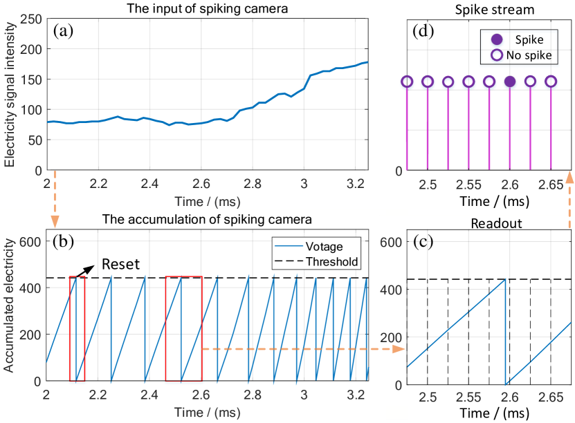
Figure 2: Illustration of the spiking camera model. (a) The input electrical signal at a pixel. (b) The accumulation corresponding to the pixel. (c) The polling readout of spikes where the spiking camera triggers the generation of spike at a frequency of 40000 Hz. (d) Generated a spike stream at the pixel.

The spiking camera mimicking the retina fovea consists of an array of $H\times W$ pixels and can report per-pixel luminance intensity by firing spikes asynchronously. Specifically, each pixel on the spiking camera sensor accumulates incoming light independently and persistently. At time $t$, for pixel $(i,j)$, if the accumulated brightness arrives a fixed threshold $\phi$ (as (1)), then a spike is fired and the corresponding accumulator is reset as shown in Fig. 2.

$$\mathbf{A}(i,j,t)=\int_{t_{i,j}^{\rm pre}}^{t}I(i,j,\tau)d\tau\geq\phi,$$ (1)

where $i,j\in\mathbb{Z},i\leq H,j\leq W,k\leq N$, $A(i,j,t)$ is the accumulated brightness at time $t$, $I(i,j,\tau)$ refers to the brightness of pixel $(i,j)$ at time $\tau$, and $t_{i,j}^{\rm pre}$ expresses the last time when a spike is fired at pixel $(i,j)$ before time $t$. If $t$ is the first time to send a spike, then $t_{i,j}^{\rm pre}$ is set as 0. In fact, due to the limitations of circuit technology, the spike reading times are quantified. Hence, asynchronous spikes are read out synchronously. Specifically, all pixels periodically check the spike flag at time $n\Delta t,n\in\mathbb{Z}$, where $\Delta t$ is a short interval of microseconds. Therefore, the output of all pixels forms a $H\times W$ binary spiking frame. As time goes on, the camera would produce a sequence of spike frames, i.e., a $H\times W\times N$ binary spike stream and can be mathematically defined as,

$$\begin{aligned} &\mathbf{S}(i,j,n\Delta t)=\\ &\begin{cases}1&\mbox{ if $\exists t\in\left((n-1)\Delta t,n\Delta t\right]$, s.t. $\mathbf{A}(i,j,t)\geq\phi$ },\\ 0&\mbox{ if $\forall t\in\left((n-1)\Delta t,n\Delta t\right]$, $\mathbf{A}(i,j,t)<\phi$ },\\ \end{cases}\end{aligned}$$ (2)

Accordingly, the average brightness of pixel $(i,j)$ between times $a$ and $b$ can be evaluated by counting the number of spikes [spikecamera], i.e.,

$$\sum\limits_{a\leq n\Delta t\leq b}\!\!\!\!\mathbf{S}(i,j,n\Delta t)\cdot\frac{\phi}{b-a}$$ (3)

3.2 Optical Flow for The Spiking Camera

Problem Statement. We use $S_{n}\in\{0,1\}^{W\times H}$ to denote the $n$ spike frame and $W_{t_{i},t_{j}}$ to denote optical flow from time $t_{i}$ to time $t_{j}$. Given a recorded binary spike stream $\{S_{n}\},n=0,1,\cdots k$ from start to end of sampling, the goal of the spiking camera optical flow estimation is to predict the optical flow $W_{t_{i},t_{j}}$ based on the spike stream.

Challenges. Supervised learning algorithms are powerful in optical flow estimation [dosovitskiy2015flownet, sun2018pwc]. However, frame-based and event-based [zhu2018ev, lee2020spike] networks are not suitable for spike streams due to the difference of their data modalities. Besides, as we discussed in the introduction, the simple solution, i.e., the images reconstructed from a spike stream are used to estimate optical flow, is unreasonable. For estimating $\mathbf{W}_{t_{i},t_{j}}$ directly from a spike stream, another simple solution is to input the spike stream $\{S_{n}\}$ between times $t_{i}$ and $t_{j}$ as a multi-channel tensor. However, in this way, the length of $\{S_{n}\}$ increases with the increasing time interval $t_{j}-t_{i}$, which is inconvenient as the input of network. To avoid the dynamic length of the spike stream, two spike streams in static temporal windows across time $t_{i}$ and time $t_{j}$ respectively can be as input. However, the easy input would be affected by motion blur caused by static temporal windows [spikecamera].
Dataset is vital for the evaluation of methods. However, there is no dataset at present for spike-based optical flow estimation. In fact, it is difficult to build real optical flow datasets for the spiking camera since sensors cannot accurately calculate the optical flow in high-speed scenes. An alternative solution is to synthesize optical flow datasets for the spiking camera. In order to synthesize valuable spike-based optical flow datasets, high-speed scenes in datasets need to be carefully designed to ensure that they can cover all kinds of motion.

4 Spiking Optical Flow Datasets

We synthesize first two large optical flow datasets for the spiking camera (SPIFT and PHM) based on our proposed the spiking camera simulator (SPCS). In this study, we regard SPIFT as the training set and PHM as the test set. Importantly, PHM includes 10 well-designed scenes with various motion which is beneficial to evaluate the generalization of models. The details are shown in Table 1.

Table 1: Detailed information of datasets.

Dataset	Category	Frame	Flow density
SPIFT-Train	100	50000	100%
SPIFT-Validation	10	5000	100%
PHM-Test	10	25100	100%

4.1 The Spiking Camera Simulator

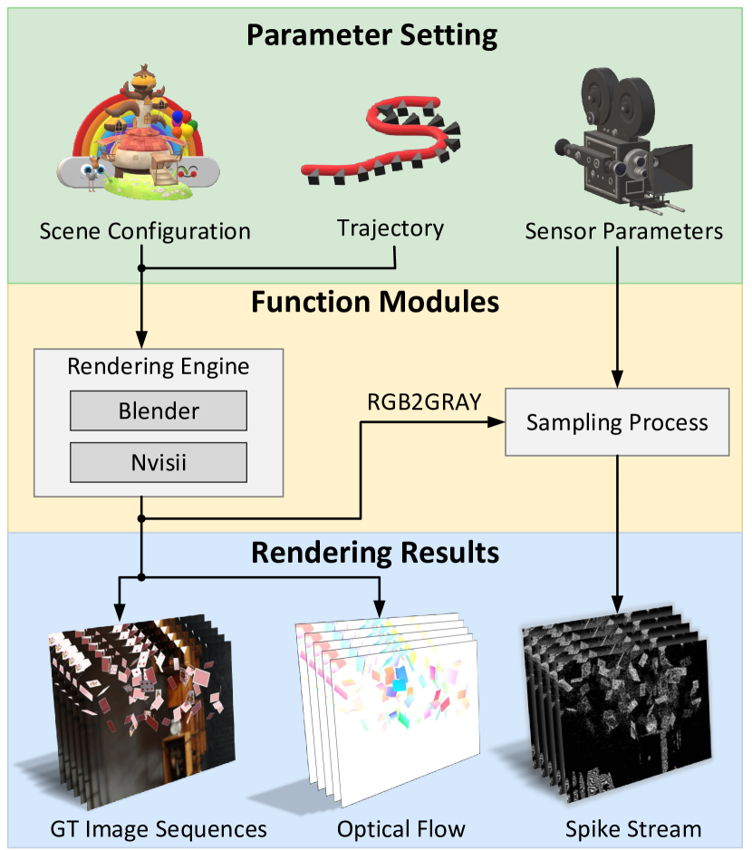
Figure 3: Framework of the spiking camera simulator, SPCS. SPCS relies on a tight coupling with the rendering engines to generate spike streams accurately. Related details are in the supplement.

To generate our datasets, we propose a simulator for the spiking camera (SPCS) coupling with rendering engines tightly. As shown in Fig. 3, its architecture mainly consists of parameter setting, rendering engine and sampling process. Parameter setting includes adding objects to the scene (scene configuration), generating the trajectory of objects (trajectory), and setting parameters of the spiking camera (sensor parameters). In SPCS, we provide a one-click generation of parameters, which means that a large number of random scenes can be easily generated. Rendering engine can be used to generate the image sequences sampled by a virtual camera in scenes. SPCS use NVISII[Morrical20nvisii] and Blender [blender] as its engine. Sampling process models the analogue circuit of the spiking camera. When SPCS generates a spike stream, image sequences would be firstly synthesized by rendering engine according to parameter settings, and then the function sampling process would convert image sequences into spike stream. Besides, for simulating sampling process more realistic, we also add noise simulation in the spiking camera.

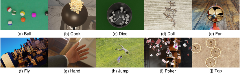
Figure 4: Scenes of Photo-realistic High-speed Motion dataset, denoted as PHM.

4.2 SPIFT Dataset

As shown in Fig. 1, each scene in the training set describes that different kinds of objects translate and rotate in random background, like FlyingChairs [dosovitskiy2015flownet], and includes spike streams with 500 frames, corresponding GT images and optical flow. Note that we do not generate optical flow at each spike frame, i.e., $\{W_{k\cdot\Delta t,(k+1)\cdot\Delta t}\}$, $\Delta t=1$, $k\in\mathbb{Z}$, since the movement of objects per spike frame is extremely small at the frame rate of spiking cameras (40000Hz). Instead of this, we generate optical flow every 10 spike frames ($\Delta t=10$) and 20 spike frames ($\Delta t=20$) separately from start to end of sampling. We hope the two sets of optical flow can be used to validate the generalization of models on motion with different magnitudes. All parameters for scenes (number, size and initial positions of objects) are randomly set to improve diversity (see supplement).

4.3 PHM Dataset

Each scene in the testing set is carefully designed and has a lot in common with the real world.

As shown in Fig. 4, “Ball” describes that billiard balls collide with each other. “Cook” describes that the vegetables are stirred in a pot. “Dice” describes the rotation of dice. “Doll” describes that some dolls fall from high onto the steps. ”Fan” describes fan blade rotation of electric fan. “Fly” describes that the Unmanned Aerial Vehicle aerial scene. “Hand” describes that an arm waves in front of the moving camera. “Jump” describes that two people tumble and jump. “Poker” describes that pokers are thrown into the air. “Top” describes that the four tops spin fast and collide.

5 Method

5.1 Spike Stream Representation

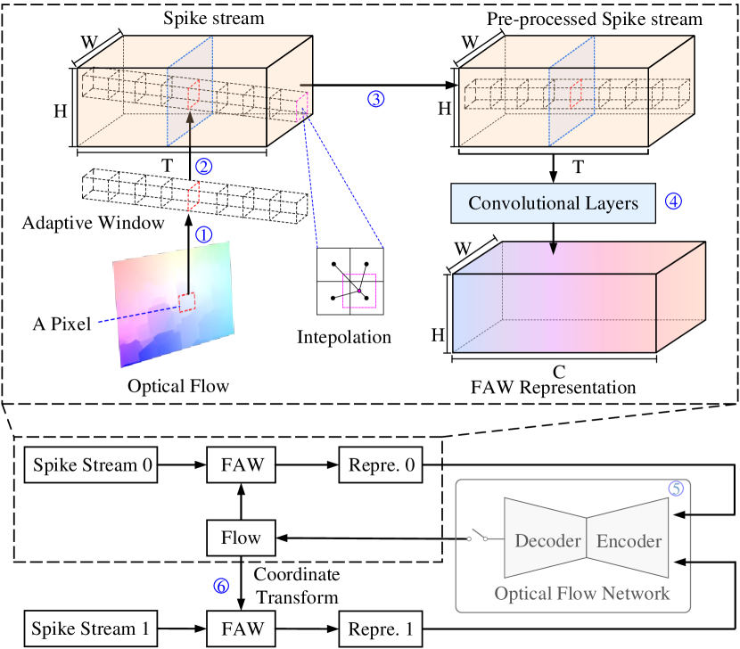
Figure 5: Architecture of proposed representation of a spike stream, FAW. The spike stream includes $T$ spike frames and each spike frame corresponds to a $H\times W$ binary array. The dimension of obtained FAW is $H\times W\times C$. Spike stream 0 (or 1) corresponds the spike stream across time $t_{0}$ (or $t_{1}$).

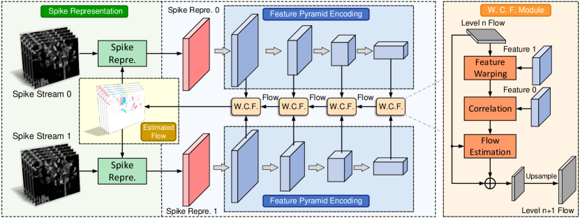
Figure 6: The network architecture of SCFlow. The spike stream is firstly represented by FAW and then constructed to be a feature pyramid. The flow is estimated through the pyramid in a coarse-to-fine manner.

An appropriate input representation of a spike stream for neural networks is crucial. In previous works [rec3, rec4], the spike stream in a temporal window with fixed direction across time $t_{0}$ is used as features at time $t_{0}$. However, the input representation would introduce motion blur due to the static temporal windows [spikecamera].

In order to reduce the influence of motion blur on representation at time $t_{0}$, selected temporal windows should be dynamic and directed. Specifically, if the direction of a temporal window is consistent with the motion trajectory of the pixel, the average brightness in the temporal window would be closer to the brightness of the pixel at time $t_{0}$. To this end, we introduce a proper representation of a spike stream, Flow-guided Adaptive Window (FAW), where prior motion is used as guidance to adaptively adjust the direction of temporal windows for each pixel. For computing FAW at time $t_{0}$, we firstly use the optical flow from time $t_{0}$ to time $t_{1}$ ($t_{1}=t_{0}+\Delta t$), $W_{t_{0},t_{1}}$ as the prior motion information of all pixels at time $t_{0}$. Furthermore, we assume that the motion of pixels is a uniform linear motion in a very short time. Hence, the adaptive temporal window of each pixel at time $t_{0}$ is straight as shown in Fig. 5②, and for the pixel $\mathbf{x}=(x,y)$, the spike information at time $t$ in its adaptive temporal window can be defined as,

$$\mathbf{S}_{t_{0}}^{\rm pre}(\mathbf{x},t)=\mathbf{S}\Big{(}\mathbf{x}+\frac{(t-t_{0})\cdot{{\mathbf{W}}}_{t_{0},t_{1}}(\mathbf{x})}{\Delta t},\;t\Big{)},$$ (4)

where $t\in[t_{0}-\frac{T_{\max}-1}{2},t_{0}+\frac{T_{\max}-1}{2}]$, $t_{1}=t_{0}+\Delta t$ and $\mathbf{S}_{t_{0}}^{\rm pre}$ is the pre-processed spike stream recording the spike information in all adaptive temporal windows, and $T_{\max}$ is the window length of the input spike stream. Note that spatial locations of the grids in adaptive temporal windows at time $t$ may not be integer, we use the bilinear interpolated spike information in the grids as shown in Fig. 5③. Further, the pre-processed spike stream at time $t_{0}$ would be encoding into a feature map with multi-channel $\mathbf{S}_{t_{0}}^{\rm FAW}$ as the FAW at time $t_{0}$ by two convolutional layers with 32 channels as shown in Fig.5④.
In fact, there is a key problem, how to obtain the prior motion (optical flow ${\mathbf{W}}_{t_{0},t_{1}}$)? As shown in Fig. 5⑤, we can use the output of Optical Flow Network (see detail of SCFlow in Section 5.2) $\hat{\mathbf{W}}_{t_{0},t_{1}}$ as prior motion. Specifically, during training, we first set prior motion as a zero matrix and a predicted optical flow can be obtained by the forward propagation of SCFlow. Then, we use the predicted optical flow as our prior motion to train SCFlow. During testing, the optical flows that need to be predicted is sorted in chronological order i.e., $\{\mathbf{W}_{k\cdot\Delta t,(k+1)\cdot\Delta t}\}$, $k\in\mathbb{N}$, $\Delta t\in\{10,20\}$. Due to high similarity of motion in adjacent time, the last predicted optical flow is used as a prior motion for the current testing i.e., the prior motion for estimating $\mathbf{W}_{i,i+\Delta t}$ is $\hat{\mathbf{W}}_{i-\Delta t,i}$.
When estimating ${\mathbf{W}}_{t_{0},t_{1}}(\mathbf{x})$, we only need to input the FAW pair at time $t_{0}$ and time $t_{1}$ to our network. However, when computing the FAW at time $t_{1}$, the key frame $\mathbf{S}(x,t_{1})$ and flow $\hat{\mathbf{W}}_{t_{0},t_{1}}$ are on different coordinates. As shown in Fig. 5⑥, we need to transform $\hat{\mathbf{W}}_{t_{0},t_{1}}$. According to the uniform linear motion assumption for the motion field, the coordinates transformation to make $\hat{\mathbf{W}}_{t_{0},t_{1}}$ aligned with spike steam at time $t_{1}$ can be written as,

$$\mathcal{C}\Big{(}{\mathbf{W}}_{t_{0},t_{1}}(\mathbf{x})\Big{)}={\mathbf{W}}_{t_{0},t_{1}}\Big{(}\mathbf{x}-{\mathbf{W}}_{t_{0},t_{1}}(\mathbf{x})\Big{)},$$ (5)

$$\mathbf{S}_{t_{1}}^{\rm pre}(\mathbf{x},t)=\mathbf{S}\Bigg{(}\mathbf{x}+\frac{(t-t_{1})\cdot\mathcal{C}\Big{(}{\mathbf{W}}_{t_{0},t_{1}}(\mathbf{x})\Big{)}}{\Delta t},\;t\Bigg{)},$$ (6)

where $t\in[t_{1}-\frac{T_{\max}-1}{2},t_{1}+\frac{T_{\max}-1}{2}]$, and $\mathcal{C}(\cdot)$ is the coordinate transformation operator.

Table 2: Average end point error comparison with other methods for estimating optical flow on PHM datasets under $\Delta t=10$ and $\Delta t=20$ settings. All methods use spike stream as input and are trained on SPIFT. The best results for each scene and the best average results are marked in bold.

	Method	Param.	Ball	Cook	Dice	Doll	Fan	Fly	Hand	Jump	Poker	Top	AVG.
$\Delta t=10$	EV-FlowNet	53.43M	0.571	3.000	0.761	1.273	0.928	11.599	5.011	0.742	1.167	2.762	3.590
	Spike-FlowNet	13.04M	0.482	3.509	0.568	0.786	0.901	12.003	4.898	0.780	0.693	2.617	3.577
	RAFT	5.40M	1.579	2.953	1.117	1.345	0.771	10.321	4.175	1.221	0.926	3.039	3.393
	SCFlow-w/oR	0.57M	0.614	1.989	1.303	0.514	0.409	9.715	2.294	0.268	1.131	2.474	2.809
	SCFlow (ours)	0.80M	0.632	1.620	1.224	0.259	0.293	9.418	1.811	0.130	0.943	2.171	2.568
$\Delta t=20$	EV-FlowNet	53.43M	1.151	5.637	1.927	1.821	1.854	22.828	9.608	0.827	2.522	5.316	6.980
	Spike-FlowNet	13.04M	0.987	7.048	1.122	3.039	1.839	25.130	9.816	1.902	1.397	5.423	7.565
	RAFT	5.40M	4.826	6.556	4.542	2.681	2.400	22.804	7.605	3.066	4.999	7.157	8.165
	SCFlow-w/oR	0.57M	1.361	3.654	2.924	1.285	0.811	20.729	4.460	0.447	2.158	4.609	5.844
	SCFlow (ours)	0.80M	1.115	3.320	2.582	0.515	0.566	20.835	4.442	0.240	1.884	4.301	5.583

5.2 Network Architecture

As shown in Fig. 6, the SCFlow network is designed in a pyramidal encoder-decoder manner. The inputs of the network are the FAW pairs. For each FAW, we build a 4-level feature pyramid $\{F_{i}^{l}(\mathbf{x})\}_{l=1}^{4},i=0,1$, which denotes the feature for describing the scene at time $t_{i}$ at $l$-th level. The feature pyramid has 32, 64, 96 and 128 channels in each level respectively.

We estimate the optical flow from higher level to lower level in pyramid. We refer to the well-known PWC-Net [sun2018pwc] to design the decoder. At $l$-th level, we firstly warp ${F}_{1}^{l}(\mathbf{S})$ via the current estimated flow $\hat{\mathbf{W}}_{t_{0},t_{1}}^{l+1}(\mathbf{S})$:

$${F}_{1,{\rm\hat{\mathbf{W}}_{t_{0},t_{1}}}}^{l}(\mathbf{x})={F}_{1}^{l}\big{(}\mathbf{x+\hat{{W}}}_{t_{0},t_{1}}^{l+1}(\mathbf{x})\big{)},$$ (7)

where we use bilinear interpolation for the warping operation. We use the features to build a correlation volume [scharstein2002taxonomy, xu2017accurate] to describe the similarity between the features. The correlation volume represents the potential displacements between the two frames, and we normalize the feature in each channel, which can be formulated as:

$$\mathbf{C}^{l}(\mathbf{x,m})=\left\langle\frac{F_{0}^{l}(\mathbf{x})-\mu_{0}^{l}}{\sigma_{0}^{l}},\frac{F_{1,{\rm w}}^{l}(\mathbf{x+m})-\mu_{1,{\rm w}}^{l}}{\sigma_{1,{\rm w}}^{l}}\right\rangle,$$ (8)

where $\mathbf{m}$ represents the displacement between the two features, $\hat{\mathbf{W}}_{t_{0},t_{1}}$ is written as $\mathbf{w}$ for simplicity and $\langle\cdot\rangle$ is the channel-wise inner product operation. $\mu$ and $\sigma$ is the mean and standard deviation value corresponding to feature with the same subscript.

The correlation and the feature extracted from the former spike stream at current level are input to the weight-shared flow estimator. A $1\times 1$ convolution is employed to adjust the channel numbers at different levels to be 32. The flow estimator consisting of cascaded convolutional layers predicts the residual flow. The refined flow is then upsampled via bilinear kernel as the final output of current level. The flow is supervised by its ground truth at each level:

$$\mathcal{L}=\sum_{l=1}^{4}\frac{HW}{2^{4-l}}\|\hat{\mathbf{W}}^{l}_{t_{0},t_{1}}-\mathbf{W}^{l}_{t_{0},t_{1}}\|_{2}^{2},$$ (9)

where $\mathcal{L}$ is our loss function, and $\mathbf{W}^{l}_{t_{0},t_{1}}$ is the ground truth of the flow at $l$-th level.

6 Experiments

Figure 7: Visual comparison of our SCFlow with other methods under the $\Delta t=10$ setting. Other visualization results are in our supplement.

6.1 Implementation Details

We train our end-to-end model on the training set of SPIFT in PyTorch. All models are trained by Adam optimizer with $\beta_{1}=0.9$ and $\beta_{2}=0.99$. We set the learning rate as 1e-4 and train 40 epochs for the $\Delta t=10$ setting and 80 epochs for the $\Delta t=20$ setting. We keep the input from SPIFT as the original 500$\times$800 resolution. The batch size in training is set as 4, and we train our models on NVIDIA Tesla A100s.

Figure 8: The optical flow visualization on PKU-Spike-High-Speed Dataset [rec1] where $\Delta t=10$ corresponds optical flow with an interval of 10 spike frames and $\Delta t=20$ corresponds optical flow with an interval of 20 spike frames. (a) A car traveling at a speed of 100 km/h (kilometers per hour). (b) A free-falling doll. (c) A high-speed rotating fan. (d) A train travelling at 350 km/h. All scenes are shot without lens movement. Other visualization results on PKU-Spike-High-Speed Dataset are in our supplement.

6.2 Comparison Results

We compare our method with three categories of methods: First, we compare our network with neural networks in event-based optical flow, i.e., EV-FlowNet [zhu2018ev] and Spike-FlowNet [lee2020spike], which are retrained in the same way as SCFlow. The Spike-FlowNet estimates optical flow in a recurrent manner, we split our spike stream to slices with length equals to 2. Second, we compare our network with state-of-the-art frame-based optical flow network, RAFT [teed2020raft], which is retrained in the same way with SCFlow. In RAFT, two spike streams in temporal windows across time $t_{0}$ and time $t_{1}$ respectively are as input instead of the images at time $t_{0}$ and $t_{1}$. Third, we compare our method with SCFlow without FAW representation (SCFlow-w/oR), which can be viewed as the ablation experiments for FAW.

Qualitative Evaluation on Proposed Datasets. We use average end point error (AEPE) as the evaluation metric, which indicates the average $\ell_{2}$ norm of the error motion vector between predicted flow and its ground truth. The quantitative comparison results are shown in Table 2. In both $\Delta t=10$ and $\Delta t=20$ settings, our SCFlow gets the best average performance in all methods with a lot fewer parameters. The comparison between SCFlow-w/oR and SCFlow demonstrates that FAW can improve the accuracy of optical flow estimation. The visualization results are shown in Fig. 7. Evidently, the EV-FlowNet[zhu2018ev], Spike-FlowNet[lee2020spike], and RAFT[teed2020raft] cannot estimate optical flow of the spiking camera well, which demonstrates the information processing pattern are not appropriate for spike streams. The flow visualization of SCFlow includes finer motion boundaries and textures than SCFlow-w/oR, which demonstrates the efficiency of the FAW representation.

Qualitative Evaluation on Real Data. In Fig. 8, we show that the visualization results of all methods on real spike streams, PKU-Spike-High-Speed Dataset [rec1]. The visual quality of optical flow produced by our proposed method is evidently better than the competing methods. For EV-FlowNet, motion region can be distinguished but predicted direction of motion is inaccurate. For Spike-FlowNet and RAFT, the boundary of predicted motion region is severely blurry. Besides, by using the FAW representation, predicted motion regions by SCFlow have the more clear boundary than SCFlow-w/oR.

7 Conclusion

This paper proposed, SCFlow, the first deep learning pipeline for optical flow estimation for the spiking camera. To avoid the motion blur in a spike stream [spikecamera] caused by static temporal windows, a proper input representation of the spike stream, Flow-guided Adaptive Window (FAW). Besides, we synthesize the two optical flow datasets for the spiking camera, SPIFT and PHM, corresponding to random high-speed and well-designed scenes respectively. Finally, we show that SCFlow can predict optical flow from real and synthetic spike streams in different high-speed scenarios.

Limitations. High-speed scenes in low light conditions may be a challenge for our model due to more obvious noise and motion blur in spike streams. In future, we plan to extend our datasets and evaluate the performance of our model on scenes in extreme lighting conditions.