Nash Convergence of Mean-Based Learning Algorithms
in First Price Auctions

Abstract

Understanding the convergence properties of learning dynamics in repeated auctions is a timely and important question in the area of learning in auctions, with numerous applications in, e.g., online advertising markets. This work focuses on repeated first price auctions where bidders with fixed values for the item learn to bid using mean-based algorithms – a large class of online learning algorithms that include popular no-regret algorithms such as Multiplicative Weights Update and Follow the Perturbed Leader. We completely characterize the learning dynamics of mean-based algorithms, in terms of convergence to a Nash equilibrium of the auction, in two senses: (1) time-average: the fraction of rounds where bidders play a Nash equilibrium approaches 1 in the limit; (2) last-iterate: the mixed strategy profile of bidders approaches a Nash equilibrium in the limit. Specifically, the results depend on the number of bidders with the highest value:

• If the number is at least three, the bidding dynamics almost surely converges to a Nash equilibrium of the auction, both in time-average and in last-iterate.

• If the number is two, the bidding dynamics almost surely converges to a Nash equilibrium in time-average but not necessarily in last-iterate.

• If the number is one, the bidding dynamics may not converge to a Nash equilibrium in time-average nor in last-iterate.

Our discovery opens up new possibilities in the study of convergence dynamics of learning algorithms.

1 Introduction

First price auctions are the current trend in online advertising auctions. A major example is Google Ad Exchange’s switch from second price auctions to first price auctions in 2019 (Paes Leme et al.,, 2020; Goke et al.,, 2022).

Compared to second price auctions, first price auctions are non-truthful: bidders need to reason about other bidders’ private values and bidding strategies and choose their own bids accordingly to maximize their utilities. Finding a good bidding strategy used to be a difficult task due to each bidder’s lack of information of other bidders. But given the repeated nature of online advertising auctions and with the advance of computing technology, nowadays’ bidders are able to learn to bid using automated bidding algorithms. As one bidder adjusts bidding strategies using a learning algorithm, other bidders’ utilities are affected and thus they will adjust their strategies as well. Then, a natural question follows: if all bidders in a repeated first price auction use some learning algorithms to adjust bidding strategies at the same time, will they converge to a Nash equilibrium of the auction?

A partial answer to this question is given by Hon-Snir et al., (1998) who show that, in a repeated first price auction where bidders have fixed values for the item, a Nash equilibrium may or may not be learned by the Fictitious Play algorithm, where in each round of auctions every bidder best responds to the empirical distributions of other bidders’ bids in history. Fictitious Play, however, is a deterministic algorithm that does not have the no-regret property — a desideratum for learning algorithms in adversarial environments. The no-regret property can only be obtained by randomized algorithms (Roughgarden,, 2016). As observed by Nekipelov et al., (2015) that bidders’ behavior on Bing’s advertising system is consistent with no-regret learning, it is hence important, from both theoretical and practical points of view, to understand the convergence property of no-regret algorithms in repeated first price auctions. This motivates our work.

Our contributions

Focusing on repeated first price auctions where bidders have fixed values, we completely characterize the Nash convergence property of a wide class of randomized online learning algorithms called “mean-based algorithms” (Braverman et al.,, 2018). This class contains most of popular no-regret algorithms, including Multiplicative Weights Update (MWU), Follow the Perturbed Leader (FTPL), etc..

We systematically analyze two notions of Nash convergence: (1) time-average: the fraction of rounds where bidders play a Nash equilibrium approaches 1 in the limit; (2) last-iterate: the mixed strategy profile of bidders approaches a Nash equilibrium in the limit. Specifically, the results depend on the number of bidders with the highest value:

• If the number is at least three, the bidding dynamics of mean-based algorithms almost surely converges to Nash equilibrium, both in time-average and in last-iterate.

• If the number is two, the bidding dynamics almost surely converges to Nash equilibrium in time-average but not necessarily in last-iterate.

• If the number is one, the bidding dynamics may not converge to Nash equilibrium in time-average nor in last-iterate.

For the last case, the non-convergence result is proved for the Follow the Leader algorithm, which is a mean-based algorithm that is not necessarily no-regret. We also show by experiments that no-regret mean-based algorithms such as MWU and $\varepsilon_{t}$-Greedy may not last-iterate converge to a Nash equilibrium.

Intuitions and techniques

The intuition behind our convergence results (the first two cases above) relates to the notion of “iterated elimination of dominated strategies” in game theory. Suppose there are three bidders all having a same integer value $v$ for the item and choosing bids from the set $\{0,1,\ldots,v-1\}$. The unique Nash equilibrium is all bidders bidding $v-1$. The elimination of dominated bids is as follows: firstly, bidding $0$ is dominated by bidding $1$ for each of the three bidders no matter what other bidders bid, so bidders will learn to bid $1$ or higher instead of bidding $0$ at the beginning; then, given that no bidders bid $0$, bidding $1$ is dominated by bidding $2$, so all bidders learn to bid at least $2$; …; in this way all bidders learn to bid $v-1$.

The above intuition is only high-level. In particular, since bidders use mean-based algorithms which may pick a dominated bid with a small but positive probability, additional argument is needed to show that bidders will finally converge to $v-1$ with high probability. To do this, we borrow and generalize a technique (which is a combination of time-partitioning and Azuma’s inequality) from Feng et al., (2021) who show that bidders in a second price auction with multiple Nash equilibria converge to the truthful equilibrium if they use mean-based algorithms with an initial uniform exploration stage. Their argument relies on the fact that, in a second price auction, all bidders learn the truthful Nash equilibrium with high probability during the uniform exploration stage. In contrast, we allow any mean-based algorithms without an initial uniform exploration stage.

1.1 Discussion

An assumption made in our work is that each bidder has a fixed value for the item sold throughout the repeated auction. Seemingly restrictive, this assumption can be justified in several aspects. First, fixed value is in fact a quite common assumption in the literature on repeated auctions, in various contexts including value inference (Nekipelov et al.,, 2015), dynamic pricing (Amin et al.,, 2013; Devanur et al.,, 2015; Immorlica et al.,, 2017), as well as the study of bidding equilibrium (Hon-Snir et al.,, 1998; Iyer et al.,, 2014; Kolumbus and Nisan,, 2022; Banchio and Skrzypacz,, 2022). An exception is the work by Feng et al., (2021) who study repeated first price auctions under the Bayesian assumption that bidders’ values are i.i.d. samples from a distribution at every round. However, their result is restricted to a $2$-symmetric-bidder setting with the Uniform$[0,1]$ distribution where the Bayesian Nash equilibrium (BNE) is simply every bidder bidding half of their values. For general asymmetric distributions there is no explicit characterization of the BNE (Lebrun,, 1996, 1999; Maskin and Riley,, 2000) despite the existence of (inefficient) numerical approximations (Fibich and Gavious,, 2003; Escamocher et al.,, 2009; Wang et al.,, 2020; Fu and Lin,, 2020). No algorithms are known to be able to compute BNE efficiently for all asymmetric distributions, let alone a simple, generic learning algorithm.

Moreover, in real-life auctions, fixed values do occur if a same item is sold repeatedly, bidders have stable values for that item, and the set of bidders is fixed. An example is a few large online travel agencies (Agoda, Airbnb, and Booking.com) competing for an ad slot about “hotel booking”. In such Internet advertising auction scenarios, a large number of auctions can happen in a short amount of time, which allows learning bidders to converge to the Nash equilibrium quickly.

Finally, as we will show, even with the seemingly innocuous assumption of fixed values, the learning dynamics of mean-based algorithms already exhibits complicated behaviors: it may converge to different equilibria in different runs or not converge at all. One can envision more unpredictable behaviors when values are not fixed.

Learning in general games

Our work is related to a fundamental question in the field of Learning in Games (Fudenberg and Levine,, 1998; Cesa-Bianchi and Lugosi,, 2006; Nisan et al.,, 2007): if players in a repeated game employ online learning algorithms to adjust strategies, will they converge to an equilibrium? And what kinds of equilibrium? Classical results include the convergence of no-regret learning algorithms to a Coarse Correlated Equilibrium (CCE) and no-internal-regret algorithms to a Correlated Equilibrium in any game (Foster and Vohra,, 1997; Hart and Mas-Colell,, 2000). But given that (coarse) correlated equilibria are much weaker than the archetypical solution concept of a Nash equilibrium, a more appealing and challenging question is the convergence towards Nash equilibrium. Positive answers to this question are only known for some special cases of algorithms and games: e.g., no-regret algorithms converge to Nash equilibria in zero-sum games, $2\times 2$ games, and routing games (Fudenberg and Levine,, 1998; Cesa-Bianchi and Lugosi,, 2006; Nisan et al.,, 2007). In contrast, several works give non-convergence examples: e.g., the non-convergence of MWU in a $3\times 3$ game (Daskalakis et al.,, 2010) and Regularized Learning Dynamics in zero-sum games (Mertikopoulos et al.,, 2017). In this work we study the Nash equilibrium convergence property in first price auctions for a large class of learning algorithms, namely the mean-based algorithms, and provide both positive and negative results.

Last v.s. average iterate convergence

We emphasize that previous results on convergence of learning dynamics to Nash equilibria in games are mostly attained in an average sense, i.e., the empirical distributions of players’ actions converge. Our notion of time-average convergence, which requires players play a Nash equilibrium in almost every round, is different from the convergence of empirical distributions; in fact, ours is stronger if the Nash equilibrium is unique. Nevertheless, time-average convergence fails to capture the full picture of the dynamics since players’ last-iterate (mixed) strategy profile may not converge. Existing results about last-iterate convergence show that most of learning dynamics actually diverge or enter a limit cycle even in a simple $3\times 3$ game (Daskalakis et al.,, 2010) or zero-sum games (Mertikopoulos et al.,, 2017), except for a few convergence examples like optimistic gradient descent/ascent in two-player zero-sum games or monotone games (Daskalakis and Panageas,, 2018; Wei et al.,, 2021; Cai et al.,, 2022). Our results and techniques, regarding the convergence of any mean-based algorithm in first price auctions, shed light on further study of last-iterate convergence in more general settings.

1.2 Additional Related Works

Online learning in auctions

A large fraction of existing works on online learning in repeated auctions are from the seller’s perspective, i.e., studying how a seller can maximize revenue by adaptively changing the rules of the auction (e.g., reservation price) over time (e.g., Blum and Hartline, (2005); Amin et al., (2013); Mohri and Medina, (2014); Cesa-Bianchi et al., (2015); Braverman et al., (2018); Huang et al., (2018); Abernethy et al., (2019); Kanoria and Nazerzadeh, (2019); Deng et al., (2020); Golrezaei et al., (2021)). We focus on the bidders’ learning problem.

Existing works from bidders’ perspective are mostly about “learning to bid”, studying on how to design no-regret algorithms for a bidder to bid in various formats of repeated auctions, including first price auctions (Balseiro et al.,, 2019; Han et al.,, 2020; Badanidiyuru et al.,, 2021), second price auctions (Iyer et al.,, 2014; Weed et al.,, 2016), and more general auctions (Feng et al.,, 2018; Karaca et al.,, 2020). Those works take the perspective of a single bidder, without considering the interaction among multiple bidders all learning to bid at the same time. We instead study the consequence of such interaction, showing that the learning dynamics of multiple bidders may or may not converge to the Nash equilibrium of the auction.

Multi-agent learning in first price auctions

In addition to the aforementioned works by Feng et al., (2021) and Hon-Snir et al., (1998), other works on multi-agent learning in first price auctions include, e.g., several empirical works by Bichler et al., (2021); Goke et al., (2022); Banchio and Skrzypacz, (2022) and a theoretical work by Kolumbus and Nisan, (2022). Bichler et al., (2021) and Banchio and Skrzypacz, (2022) observe convergence results for some learning algorithms experimentally. Kolumbus and Nisan, (2022) prove that in repeated first price auctions with two mean-based learning bidders, if the dynamics converge to some limit, then this limit must be a CCE in which the bidder with the higher value submits bids that are close to the lower value. However, they do not give conditions under which the dynamics converge. We prove that the dynamics converge if the two bidders have the same value and in fact converge to the stronger notion of a Nash equilibrium. This result complements Kolumbus and Nisan, (2022) and supports the aforementioned empirical findings.

Learning to iteratively eliminate dominated strategies

Although it is not surprising that mean-based learning algorithms are able to iteratively eliminate dominated strategies in repeated games, it is surprising that we cannot find a formal proof for this result in the literature. Part of the reason could be that mean-based algorithms can be randomized and difficult to analyze. As mentioned in the Introduction, we generalize a “time-partitioning” technique in Feng et al., (2021) to overcome this difficulty and give a formal proof for this result. Some recent works on multi-agent learning in other games (e.g., Wu et al., (2022); Feng et al., (2022)) also make the observation that many algorithms similar to mean-based algorithms can iteratively eliminate dominated strategies. But interestingly, Wu et al., (2022) find that those algorithms may need an exponential time to iteratively eliminated all dominated strategies in some special games. We do not know the exact convergence rate of mean-based algorithms in our first price auction game.

Organization of the paper

We discuss model and preliminaries in Section 2 and present our main results in Section 3. In Section 4 we present the proof of Theorem 4, which covers the main ideas and proof techniques of all our convergence results. Section 5 includes experimental results. We conclude and discuss future directions in Section 6. Missing proofs from Section 3 and 4 are in Appendix A and B respectively.

2 Model and Preliminaries

Repeated first price auctions

We consider repeated first-price sealed-bid auctions where a single seller sells a good to a set of $N\geq 2$ players (bidders) $\mathcal{N}=\{1,2,...,N\}$ for infinite rounds. Each player $i\in\mathcal{N}$ has a fixed private value $v^{i}$ for the good throughout. See Section 1.1 for a discussion on this assumption. We assume that $v^{i}$ is a positive integer in some range $\{1,\ldots,V\}$ where $V$ is an upper bound on $v^{i}$. Suppose $V\geq 3$. No player knows other players’ values. Without loss of generality, assume $v^{1}\geq v^{2}\geq\cdots\geq v^{N}$.

At each round $t\geq 1$ of the repeated auctions, each bidder $i$ submits a bid $b^{i}_{t}\in\{0,1,\ldots,V\}$ to compete for the good. A discrete set of bids captures the reality that the minimum unit of money is a cent. The bidder with the highest bid wins the good. If there are more than one highest bidders, the good is allocated to one of them uniformly at random. The bidder who wins the good pays her bid $b^{i}_{t}$, obtaining utility $v^{i}-b^{i}_{t}$; other bidders obtain utility $0$. Let $u^{i}(b^{i}_{t},\bm{b}^{-i}_{t})$ denote bidder $i$’s (expected) utility when $i$ bids $b^{i}_{t}$ while other bidders bid $\bm{b}^{-i}_{t}=(b^{1}_{t},\ldots,b^{i-1}_{t},b^{i+1}_{t},\ldots,b^{N}_{t})$, i.e., $u^{i}(b^{i}_{t},\bm{b}^{-i}_{t})=(v^{i}-b^{i}_{t})\mathbb{I}[b^{i}_{t}=\max_{j\in\mathcal{N}}b^{j}_{t}]\frac{1}{|\operatorname*{argmax}_{j\in\mathcal{N}}b^{j}_{t}|}$.

We assume that bidders never bid above or equal to their values since that brings them negative or zero utility, which is clearly dominated by bidding $0$. We denote the set of possible bids of each bidder $i$ by $\mathcal{B}^{i}=\{0,1,\ldots,v^{i}-1\}$.

Online learning

We assume that each bidder $i\in\mathcal{N}$ chooses her bids using an online learning algorithm. Specifically, we regard the set of possible bids $\mathcal{B}^{i}$ as a set of actions (or arms). At each round $t$, the algorithm picks (possibly in a random way) an action $b^{i}_{t}\in\mathcal{B}^{i}$ to play, and then receives some feedback. The feedback may include the rewards (i.e., utilities) of all possible actions in $\mathcal{B}^{i}$ (in the experts setting) or only the reward of the chosen action $b^{i}_{t}$ (in the multi-arm bandit setting). With feedback, the algorithm updates its choice of actions in future rounds. We do not assume a specific feedback model in this work. Our analysis will apply to all online learning algorithms that satisfy the following property, called “mean-based” (Braverman et al.,, 2018; Feng et al.,, 2021), which roughly says that the algorithm picks actions with low average historical rewards with low probabilities.

Definition 1 (mean-based algorithm).

Let $\alpha_{t}^{i}(b)$ be the average reward of action $b$ in the first $t$ rounds: $\alpha_{t}^{i}(b)=\frac{1}{t}\sum_{s=1}^{t}u^{i}(b,\bm{b}^{-i}_{s})$. An algorithm is $\gamma_{t}$-mean-based if, for any $b\in\mathcal{B}^{i}$, whenever there exists $b^{\prime}\in\mathcal{B}^{i}$ such that $\alpha_{t-1}^{i}(b^{\prime})-\alpha_{t-1}^{i}(b)>V\gamma_{t}$, the probability that the algorithm picks $b$ at round $t$ is at most $\gamma_{t}$. An algorithm is mean-based if it is $\gamma_{t}$-mean-based for some decreasing sequence $(\gamma_{t})_{t=1}^{\infty}$ such that $\gamma_{t}\to 0$ as $t\to\infty$.

In this work, we assume that the online learning algorithm may run for an infinite number of rounds. This captures the scenario where bidders do not know how long they will be in the auction and hence use learning algorithms that work for an arbitrary unknown number of rounds. Infinite-round mean-based algorithms can be obtained by modifying classical finite-round online learning algorithms (e.g., MWU) with constant learning rates to have decreasing learning rates, as shown below:

Example 2.

Let $(\varepsilon_{t})_{t=1}^{\infty}$ be a decreasing sequence approaching $0$. The following algorithms are mean-based:

• Follow the Leader (or Greedy): at each round $t\geq 1$, each player $i\in\mathcal{N}$ chooses an action $b\in\operatorname*{argmax}_{b\in\mathcal{B}^{i}}\{\alpha_{t-1}^{i}(b)\}$ (with a specific tie-breaking rule).

• $\varepsilon_{t}$-Greedy: at each round $t\geq 1$, each player $i\in\mathcal{N}$ with probability $1-\varepsilon_{t}$ chooses $b\in\operatorname*{argmax}_{b\in\mathcal{B}^{i}}\{\alpha_{t-1}^{i}(b)\}$, with probability $\varepsilon_{t}$ chooses an action in $\mathcal{B}^{i}$ uniformly at random.

• Multiplicative Weights Update (MWU): at each round $t\geq 1$, each player $i\in\mathcal{N}$ chooses each action $b\in\mathcal{B}^{i}$ with probability $\frac{w_{t-1}(b)}{\sum_{b^{\prime}\in\mathcal{B}^{i}}w_{t-1}(b^{\prime})}$, where $w_{t}(b)=\exp(\varepsilon_{t}\sum_{s=1}^{t}u^{i}(b,\bm{b}_{s}^{-i}))$.

Clearly, Follow the Leader is $(\gamma_{t}=0)$-mean-based and $\varepsilon_{t}$-Greedy is $\varepsilon_{t}$-mean-based. One can see Braverman et al., (2018) for why MWU is mean-based. Additionally, MWU is no-regret when the sequence $(\varepsilon_{t})_{t=1}^{\infty}$ is set to $\varepsilon_{t}=O(1/\sqrt{t})$ (see, e.g., Theorem 2.3 in Cesa-Bianchi and Lugosi, (2006)).

Equilibria in first price auctions

Before presenting our main results, we characterize the set of all Nash equilibria in the first price auction where bidders have fixed values $v^{1}\geq v^{2}\geq\cdots\geq v^{N}$. We only consider pure-strategy Nash equilibria in this work. Reusing the notation $u^{i}(\cdot)$, we denote by $u^{i}(b^{i},\bm{b}^{-i})$ the utility of bidder $i$ when she bids $b^{i}$ while others bid $\bm{b}^{-i}=(b^{1},\ldots,b^{i-1},b^{i+1},\ldots,b^{N})$. A bidding profile $\bm{b}=(b^{1},\ldots,b^{N})=(b^{i},\bm{b}^{-i})$ is called a Nash equilibrium if $u^{i}(\bm{b})\geq u^{i}(b^{\prime},\bm{b}^{-i})$ for any $b^{\prime}\in\mathcal{B}^{i}$ and any $i\in\mathcal{N}$. Let $M^{i}$ denote the set of bidders who have the same value as bidder $i$, $M^{i}=\{j\in\mathcal{N}:v^{j}=v^{i}\}$. $M^{1}$ is the set of bidders with the highest value.

Proposition 3.

The set of (pure-strategy) Nash equilibria in the first price auctions with fixed values $v^{1}\geq v^{2}\geq\cdots\geq v^{N}$ are bidding profiles $\bm{b}=(b^{1},\ldots,b^{N})$ that satisfy the following:

• The case of $|M^{1}|\geq 3$: $b^{i}=v^{1}-1$ for $i\in M^{1}$ and $b^{j}\leq v^{1}-2$ for $j\notin M^{1}$.

• The case of $|M^{1}|=2$:

  • If $N=2$ or $v^{1}=v^{2}>v^{3}+1$: there are two types of Nash equilibria: (1) $b^{1}=b^{2}=v^{1}-1$, with $b^{j}\leq v^{1}-3$ for $j\notin M^{1}$; (2) $b^{1}=b^{2}=v^{1}-2$, with $b^{j}\leq v^{1}-3$ for $j\notin M^{1}$.

  • If $N>2$ and $v^{1}=v^{2}=v^{3}+1$: $b^{1}=b^{2}=v^{1}-1$ and $b^{j}\leq v^{1}-2$ for $j\notin M^{1}$.

• The case of $|M^{1}|=1$:

  • Bidding profiles that satisfy the following are Nash equilibria: $b^{1}=v^{2}$, at least one bidder in $M^{2}$ bids $v^{2}-1$, all other bidders bid $b^{j}\leq v^{2}-1$.

  • If $v^{1}=v^{2}+1$ and $|M^{2}|=1$, then there is another type of Nash equilibria: $b^{1}=b^{2}=v^{2}-1$, $b^{j}\leq v^{2}-2$ for $j\notin\{1,2\}$.

There are no other (pure-strategy) Nash equilibria.

The proof of this proposition is straightforward and omitted. Intuitively, whenever more than one bidder has the highest value ($|M^{1}|\geq 2$), they should compete with each other by bidding $v^{1}-1$ (or $v^{1}-2$ if $|M^{1}|=2$ and no other bidders are able to compete with them). When $|M^{1}|=1$, the unique highest-value bidder (bidder $1$) competes with the second-highest bidders ($M^{2}$).

3 Main Results: Convergence of Mean-Based Algorithms

We introduce some additional notations. Let $\bm{x}^{i}_{t}\in\mathbb{R}^{v^{i}}$ be the mixed strategy of player $i$ in round $t$, where the $b$-th component of $\bm{x}^{i}_{t}$ is the probability that player $i$ bids $b\in\mathcal{B}^{i}$ in round $t$. The sequence $(\bm{x}^{i}_{t})_{t=1}^{\infty}$ is a stochastic process, where the randomness for each $\bm{x}^{i}_{t}$ includes the randomness of bidding by all players in previous rounds. Let $\bm{1}_{b}=(0,...,0,1,0,...,0)$ where $1$ is in the $b$-th position.

Our main results about the convergence of mean-based algorithms in repeated first price auctions depend on how many bidders have the highest value, $|M^{1}|$.

The case of $|M^{1}|\geq 3$.

Theorem 4.

If $|M^{1}|\geq 3$ and every bidder follows a mean-based algorithm, then, with probability $1$, both of the following events happen:

• Time-average convergence of bid sequence:

  $$\lim_{t\to\infty}\frac{1}{t}\sum_{s=1}^{t}\mathbb{I}[\forall i\in M^{1},b_{s}^{i}=v^{1}-1]=1.$$ (1)

• Last-iterate convergence of mixed strategy profile:

  $$\forall i\in M^{1},~{}\lim_{t\to\infty}\bm{x}^{i}_{t}=\bm{1}_{v^{1}-1}.$$ (2)

Theorem 4 can be interpreted as follows. According to Proposition 3, the bidding profile $\bm{b}_{s}$ at round $s$ is a Nash equilibrium if and only if $\forall i\in M^{1},b_{s}^{i}=v^{1}-1$ (bidders not in $M^{1}$ bid $\leq v^{1}-2$ by assumption). Hence, the first result of Theorem 4 implies that the fraction of rounds where bidders play a Nash equilibrium approaches $1$ in the limit. The second result shows that all bidders $i\in M^{1}$ bid $v^{1}-1$ with certainty eventually, achieving a Nash equilibrium.

The case of $|M^{1}|=2$.

Theorem 5.

If $|M^{1}|=2$ and every bidder follows a mean-based algorithm, then, with probability $1$, one of the following two events happens:

• $\lim_{t\to\infty}\frac{1}{t}\sum_{s=1}^{t}\mathbb{I}[\forall i\in M^{1},\ b_{s}^{i}=v^{1}-2]=1$;

• $\lim_{t\to\infty}\frac{1}{t}\sum_{s=1}^{t}\mathbb{I}[\forall i\in M^{1},b_{s}^{i}=v^{1}-1]=1$ and $\forall i\in M^{1}$, $\lim_{t\to\infty}\bm{x}_{t}^{i}=\bm{1}_{v^{1}-1}$.

Moreover, if $N>2$ and $v^{3}=v^{1}-1$ then only the second event happens.

For the case $v^{3}<v^{1}-1$, according to Proposition 3, $\bm{b}_{s}$ is a Nash equilibrium if and only if both bidders in $M^{1}$ play $v^{1}-1$ or $v^{1}-2$ at the same time (with other bidders bidding $\leq v^{1}-3$ by assumption7). Hence, the theorem shows that the bidders eventually converge to one of the two possible types of equilibria. Interestingly, experiments show that some mean-based algorithms lead to the equilibrium of $v^{1}-1$ while some lead to $v^{1}-2$. Also, a same algorithm may converge to different equilibria in different runs. See Section 5 for details.

In the case of time-average convergence to the equilibrium of $v^{1}-2$, the last-iterate convergence result does not always holds. Consider an example with 2 bidders, with $v^{1}=v^{2}=3$. We can construct a $\gamma_{t}$-mean-based algorithm with $\gamma_{t}=O(\frac{1}{t^{1/4}})$ such that, with constant probability, it holds $\lim_{t\to\infty}\frac{1}{t}\sum_{s=1}^{t}\mathbb{I}[\forall i\in M^{1},\ b_{s}^{i}=v^{1}-2]=1$ but in infinitely many rounds we have $\bm{x}_{t}^{i}=\bm{1}_{2}=\bm{1}_{v^{1}-1}$. The key idea is that, when $\alpha_{t}^{i}(1)-\alpha_{t}^{i}(2)$ is positive but lower than $V\gamma_{t}$ in some round $t$ (which happens infinitely often), we can let the algorithm bid $2$ with certainty in round $t+1$. This does not violate the $\gamma_{t}$-mean-based property.

Proposition 6.

If $|M^{1}|=2$, then there exists a mean-based algorithm such that, when players follow this algorithm, with constant probability their mixed strategy profiles do not converge to a Nash equilibrium in last-iterate.

The case of $|M^{1}|=1$.

The dynamics may not converge to a Nash equilibrium of the auction in time-average nor in last-iterate, as shown in the following example (see Appendix A for a proof).

Example 7.

Let $v^{1}=10$, $v^{2}=v^{3}=7$. Assume that players use the Follow the Leader algorithm (which is $0$-mean-based) with a specific tie-breaking rule. They may generate the following bidding path $(b_{t}^{1},b_{t}^{2},b_{t}^{3})_{t\geq 1}$:

$$(7,6,1),(7,1,6),(7,1,1),(7,6,1),(7,1,6),(7,1,1),\ldots$$

Note that $(7,1,1)$ is not a Nash equilibrium according to Proposition 3 but it appears in $\frac{1}{3}$ fraction of rounds, which means that the dynamics neither converges in the time-average sense nor in the last-iterate sense to a Nash equilibrium.

Example 7 also shows that, in the case of $|M^{1}|=1$, the bidding dynamics generated by a mean-based algorithm may not converge to Nash equilibrium in the classical sense of “convergence of empirical distribution”: i.e., letting $p_{t}^{i}=\frac{1}{t}\sum_{s=1}^{t}\bm{1}_{b_{s}^{i}}\in\Delta(\mathcal{B}^{i})$ denote the empirical distribution of player $i$’s bids up to round $t$, the vector of individual empirical distributions $(p_{t}^{1},p_{t}^{2},p_{t}^{3})_{t\geq 1}$ approaches a (mixed-strategy) Nash equilibrium in the limit. To see this, note that the vector of individual empirical distributions converges to $(p^{1},p^{2},p^{3})$ where $p^{1}(7)=1$ and for $i=2,3$, $p^{i}(6)=\frac{1}{3}$ and $p^{i}(1)=\frac{2}{3}$. It is easy to verify that for bidder $1$, bidding $2$ has utility $(10-2)(\frac{2}{3})^{2}=\frac{32}{9}$, which is larger than the utility of bidding $7$, which is $10-7=3$. Thus, $(p^{1},p^{2},p^{3})$ is not a Nash equilibrium.

The mean-based algorithm in Example 7 is not no-regret. In Section 5 we show by experiments that such non-convergence results also hold for no-regret mean-based algorithms, e.g., MWU.

4 Proof of Theorem 4

The proof of Theorem 4 covers the main ideas and proof techniques of our convergence results, so we present it here. We first provide a proof sketch. Then in Section 4.1 we provide properties of mean-based algorithms that will be used in the formal proof. Section 4.2 and Section 4.3 prove Theorem 4.

Proof sketch

The idea of the proof resembles the notion of iterative elimination of dominated strategies in game theory. We first use a step-by-step argument to show that bidders with the highest value (i.e., those in $M^{1}$) will gradually learn to avoid bidding $0,1,\ldots,v^{1}-3$. Then we further prove that: if $|M^{1}|=3$, they will avoid $v^{1}-2$ and hence converge to $v^{1}-1$; if $|M^{1}|=2$, the two bidders may end up playing $v^{1}-1$ or $v^{1}-2$.

To see why bidders in $M^{1}$ will learn to avoid $0$, suppose that there are two bidders in total and one of them (say, bidder $i$) bids $b$ with probability $P(b)$ in history. For the other bidder (say, bidder $j$), if bidder $j$ bids $0$, she obtains utility $\alpha(0)=(v^{1}-0)\frac{P(0)}{2}$; if she bids $1$, she obtains utility $\alpha(1)=(v^{1}-1)(P(0)+\frac{P(1)}{2})$. Since $\alpha(1)-\alpha(0)=\frac{v^{1}-2}{2}P(0)+(v^{1}-1)\frac{P(1)}{2}>0$ (assuming $v^{1}\geq 3$), bidding $1$ is better than bidding $0$ for bidder $j$. Given that bidder $j$ is using a mean-based algorithm, she will play $0$ with small probability (say, zero probability). The same argument applies to bidder $i$. Hence, both bidders learn to not play $0$. Then we take an inductive step: assuming that no bidders play $0,\ldots,k-1$, we note that $\alpha(k+1)-\alpha(k)=\frac{v^{1}-k-2}{2}P(k)+\frac{v^{1}-k-1}{2}P(k+1)>0$ for $k\leq v^{1}-3$, therefore $k+1$ is a better response than $k$ and both players will avoid bidding $k$. An induction shows that they will finally learn to avoid $0,1,\ldots,v^{1}-3$. Then, for the case of $|M^{1}|\geq 3$, we will use an additional claim (Claim 9) to show that, if bidders bid $0,1,\ldots,v^{1}-3$ rarely in history, they will also avoid bidding $v^{1}-2$ in the future.

The formal proof uses a time-partitioning technique proposed by Feng et al., (2021). Roughly speaking, we partition the time horizon into some periods $1<T_{0}<T_{1}<T_{2}<\cdots$. If bidders bid $0,1,\ldots,k-1$ with low frequency from round $1$ to $T_{k-1}$, then using the mean-based properties in Claim 8 and Claim 9, we show that they will bid $k$ with probability at most $\gamma_{t}$ in each round from $T_{k-1}+1,T_{k-1}+2,\ldots,$ to $T_{k}$. A use of Azuma’s inequality shows that the frequency of bid $k$ in period $(T_{k-1},T_{k}]$ is also low with high probability, which concludes the induction. Constructing an appropriate partition allows us to argue that the frequency of bids less than $v^{1}-1$ converges to $0$ with high probability.

4.1 Properties of Mean-Based Algorithms in First Price Auctions

We use the following notations intensively in the proofs. We denote by $P_{t}^{i}(k)$ the frequency of the highest bid submitted by bidders other than $i$ during the first $t$ rounds:

$$P_{t}^{i}(k)=\tfrac{1}{t}\textstyle\sum_{s=1}^{t}\mathbb{I}[\max_{j\neq i}b_{s}^{j}=k].$$

By $P_{t}^{i}(0:k)$ we mean $\sum_{\ell=0}^{k}P_{t}^{i}(\ell)$. Let $P_{t}^{i}(0:-1)$ be $0$. Additionally, let $Q_{t}^{i}(k)$ be the probability of bidder $i$ winning the item with ties if she bids $k$ in history:

$$Q_{t}^{i}(k)=\tfrac{1}{t}\textstyle\sum_{s=1}^{t}\mathbb{I}[\max_{j\neq i}b_{s}^{j}=k]\frac{1}{|\operatorname*{argmax}_{j\neq i}b_{s}^{j}|+1}.$$

Clearly,

$$0\leq\tfrac{1}{N}P_{t}^{i}(k)\leq Q_{t}^{i}(k)\leq\tfrac{1}{2}P_{t}^{t}(k)\leq\tfrac{1}{2}.$$ (3)

We can use $P_{t}^{i}(0:k-1)$ and $Q_{i}^{t}(k)$ to express $\alpha_{t}^{i}(k)$:

$$\alpha_{t}^{i}(k)=(v^{i}-k)\big{(}P_{t}^{i}(0:k-1)+Q_{t}^{i}(k)\big{)}.$$ (4)

We use $H_{t}$ to denote the history of the first $t$ rounds, which includes the realization of all randomness in the first $t$ rounds. Bidders themselves do not necessarily observe the full history $H_{t}$. Given $H_{t-1}$, each bidder’s mixed strategy $\bm{x}_{t}^{i}$ at round $t$ is determined, and the $k$-th component of $\bm{x}_{t}^{i}$ is exactly $\Pr[b_{t}^{i}=k\mid H_{t-1}]$. The following claim says that, if other bidders rarely bid $0$ to $k-1$ in history, then bidder $i$ will not bid $k$ with large probability in round $t$, for $i\in M^{1}$.

Claim 8.

Assume $v^{1}\geq 3$. For any $i\in M^{1}$, any $k\in\{0,1,\ldots,v^{1}-3\}$, any $t\geq 1$, if the history $H_{t-1}$ of the first $t-1$ rounds satisfies $P_{t-1}^{i}(0:k-1)<\frac{1}{2VN}-2\gamma_{t}$, then $\Pr[b_{t}^{i}=k\mid H_{t-1}]\leq\gamma_{t}$.

Proof.

Suppose $P_{t-1}^{i}(0:k-1)\leq\frac{1}{2VN}-2\gamma_{t}$ holds. If $\alpha_{t-1}^{i}(k+1)-\alpha_{t-1}^{i}(k)>V\gamma_{t}$, then by the mean-based property, the conditional probability $\Pr[b_{t}^{i}=k\mid\alpha_{t-1}^{i}(k+1)-\alpha_{t-1}^{i}(k)>V\gamma_{t},H_{t-1}]$ is at most $\gamma_{t}$. Otherwise, we have $\alpha_{t-1}^{i}(k+1)-\alpha_{t-1}^{i}(k)\leq V\gamma_{t}$. Using (4) and (3),

$$V\gamma_{t} \geq\alpha_{t-1}^{i}(k+1)-\alpha_{t-1}^{i}(k)$$

$$\geq(v^{1}-k-1)P_{t-1}^{i}(k)-P_{t-1}^{i}(0:k-1)-(v^{1}-k)\tfrac{P_{t-1}^{i}(k)}{2},$$

which implies

$$P_{t-1}^{i}(k)\leq\tfrac{2}{v^{1}-k-2}\big{(}V\gamma_{t}+P_{t-1}^{i}(0:k-1)\big{)}.$$ (5)

We then upper bound $\alpha_{t-1}^{i}(k)$ by

$$\alpha_{t-1}^{i}(k) \leq(v^{1}-k)\big{(}P_{t-1}^{i}(0:k-1)+\tfrac{1}{2}P_{t-1}^{i}(k)\big{)}$$

by (5) $$\leq(v^{1}-k)P_{t-1}^{i}(0:k-1)+\tfrac{v^{1}-k}{v^{1}-k-2}\big{(}V\gamma_{t}+P_{t-1}^{i}(0:k-1)\big{)}$$

$$=\tfrac{v^{1}-k}{v^{1}-k-2}V\gamma_{t}+\big{(}v^{1}-k+\tfrac{v^{1}-k}{v^{1}-k-2}\big{)}P_{t-1}^{i}(0:k-1)$$

($$\tfrac{v^{1}-k}{v^{1}-k-2}\leq 3 \leq 3V\gamma_{t}+\big{(}v^{1}-k+3\big{)}P_{t-1}^{i}(0:k-1)$$)

$$\leq 3V\gamma_{t}+2VP_{t-1}^{i}(0:k-1).$$

By the assumption that $P_{t-1}^{i}(0:k-1)<\frac{1}{2VN}-2\gamma_{t}$,

$$\alpha_{t-1}^{i}(k)<3V\gamma_{t}+2V\left(\tfrac{1}{2VN}-2\gamma_{t}\right)=\tfrac{1}{N}-V\gamma_{t}.$$

Then, we note that $\alpha_{t-1}^{i}(v^{1}-1)=P_{t-1}^{i}(0:v^{1}-2)+Q_{t-1}^{i}(v^{1}-1)\geq\frac{1}{N}P_{t-1}^{i}(0:v^{1}-1)=\frac{1}{N}\cdot 1$ where the last equality holds because no bidder bids above $v^{1}-1$ by assumption. Therefore,

$$\alpha_{t-1}^{i}(v^{1}-1)-\alpha_{t-1}^{i}(k)>\tfrac{1}{N}-\left(\tfrac{1}{N}-V\gamma_{t}\right)=V\gamma_{t}.$$

From the mean-based property, $\Pr[b_{t}^{i}=k\mid\alpha_{t-1}^{i}(k+1)-\alpha_{t-1}^{i}(k)\leq V\gamma_{t},H_{t-1}]\leq\gamma_{t}$, implying $\Pr[b_{t}^{i}=k\mid H_{t-1}]\leq\gamma_{t}$. ∎

The following claim is for the case of $k=v^{1}-2$: if bidders rarely bid $0$ to $v^{1}-3$ in history, then bidder $i$ will not bid $v^{1}-2$ with large probability in round $t$, for $i\in M^{1}$, given $|M^{1}|\geq 3$.

Claim 9.

Suppose $|M^{1}|\geq 3$ and $v^{1}\geq 2$. For any $t\geq 1$ such that $\gamma_{t}<\frac{1}{12N^{2}V^{2}}$, if the history $H_{t-1}$ of the first $t-1$ rounds satisfies $\frac{1}{t-1}\sum_{s=1}^{t-1}\mathbb{I}[\exists i\in M^{1},b_{s}^{i}\leq v^{1}-3]\leq\frac{1}{3NV}$, then, $\forall$ $i\in M^{1}$, $\Pr[b_{t}^{i}=v^{1}-2\mid H_{t-1}]\leq\gamma_{t}$.

4.2 Iteratively Eliminating Bids $0,1,\ldots,v^{1}-3$

In this subsection we show that, after a sufficiently long time, bidders in $M^{1}$ will rarely bid $0,1,\ldots,v^{1}-3$, with high probability (Corollary 13). We show this by partitioning the time horizon into $v^{1}-3$ periods and using an induction from $0$ to $v^{1}-3$. Let constants $c=1+\frac{1}{12NV}$ and $d=\lceil\log_{c}(8NV)\rceil$. Let $T_{b}$ be any (constant) integer such that $\gamma_{T_{b}}<\frac{1}{12N^{2}V^{2}}$ and $\exp\left(-\frac{(c-1)T_{b}}{1152N^{2}V^{2}}\right)\leq\frac{1}{2}$. Let $T_{0}=12NVT_{b}$ and $T_{k}=c^{d}T_{k-1}=c^{dk}T_{0}\geq(8NV)^{k}T_{0}$ for $k\in\{1,2,\cdots,v^{1}-3\}$. Let $A_{k}$ be event

$$A_{k}=\left[\frac{1}{T_{k}}\sum_{t=1}^{T_{k}}\mathbb{I}[\exists i\in M^{1},b_{t}^{i}\leq k]\leq\frac{1}{4NV}\right],$$

which says that bidders in $M^{1}$ bid $0,1,\ldots,k$ not too often in the first $T_{k}$ rounds. Our goal is to show that $\Pr[A_{v^{1}-3}]$ is high.

Lemma 10.

$\Pr{\mathchoice{\left[A_{0}\right]}{[A_{0}]}{[A_{0}]}{[A_{0}]}}\geq 1-\exp\left(-\frac{T_{b}}{24NV}\right)$.

Proof.

Consider any round $t\geq T_{b}$. For any $i\in M^{1}$, given any history $H_{t-1}$ of the first $t-1$ rounds, it holds that $P_{t-1}^{i}(0:-1)=0\leq\frac{1}{2VN}-2\gamma_{t}$. Hence, by Claim 8,

$$\Pr[b_{t}^{i}=0\mid H_{t-1}]\leq\gamma_{t}.$$

Using a union bound over $i\in M^{1}$,

$$\Pr[\exists i\in M^{1},b_{t}^{i}=0\mid H_{t-1}]\leq|M^{1}|\gamma_{t}.$$

Let $Z_{t}=\mathbb{I}[\exists i\in M^{1},b_{t}^{i}=0]-|M^{1}|\gamma_{t}$ and let $X_{t}=\sum_{s=T_{b}+1}^{t}Z_{s}$. We have ${\mathbb{E}}{\mathchoice{\left[Z_{t}\mid H_{t-1}\right]}{[Z_{t}\mid H_{t-1}]}{[Z_{t}\mid H_{t-1}]}{[Z_{t}\mid H_{t-1}]}}\leq 0$. Therefore, the sequence $X_{T_{b}+1},X_{T_{b}+2},\ldots,X_{T_{0}}$ is a supermartingale (with respect to the sequence of history $H_{T_{b}},H_{T_{b}+1},\ldots,H_{T_{0}-1}$). By Azuma’s inequality, for any $\Delta>0$, we have

$$\Pr\bigg{[}\sum_{t=T_{b}+1}^{T_{0}}Z_{t}\geq\Delta\bigg{]}\leq\exp\left(-\frac{\Delta^{2}}{2(T_{0}-T_{b})}\right).$$

Let $\Delta=T_{b}$. We have with probability at least $1-\exp\left(-\frac{\Delta^{2}}{2(T_{0}-T_{b})}\right)\geq 1-\exp\left(-\frac{T_{b}}{24NV}\right)$, $\sum_{t=T_{b}+1}^{T_{0}}Z_{t}<T_{b}$, or $\sum_{t=T_{b}+1}^{T_{0}}\mathbb{I}[\exists i\in M^{1},b_{t}^{i}=0]<T_{b}+\sum_{t=T_{b}+1}^{T_{0}}|M^{1}|\gamma_{t}$, which implies

$$\frac{1}{T_{0}}\sum_{t=1}^{T_{0}}\mathbb{I}[\exists i\in M^{1},b_{t}^{i}=0] \leq\frac{1}{T_{0}}\bigg{(}T_{b}+\sum_{t=T_{b}+1}^{T_{0}}\mathbb{I}[\exists i\in M^{1},b_{t}^{i}=0]\bigg{)}$$

$$<\frac{1}{T_{0}}\bigg{(}2T_{b}+\sum_{t=T_{b}+1}^{T_{0}}|M^{1}|\gamma_{t}\bigg{)}\leq\frac{1}{4NV},$$

where the last inequality holds due to $\frac{T_{b}}{T_{0}}=\frac{1}{12NV}$ and $\frac{1}{T_{0}}\sum_{t=T_{b}+1}^{T_{0}}|M^{1}|\gamma_{t}\leq|M^{1}|\gamma_{T_{b}}\leq\frac{1}{12NV}$. ∎

The following lemma says that, if bidders in $M^{1}$ seldom bid $0,1,\ldots,k$ in the first $T_{k}$ rounds, then they will also seldom bid $0,1,\ldots,k,k+1$ in the first $T_{k+1}$ rounds, with high probability.

Lemma 11.

Suppose $|M^{1}|\geq 2$. $\Pr{\mathchoice{\left[A_{k+1}\mid A_{k}\right]}{[A_{k+1}\mid A_{k}]}{[A_{k+1}\mid A_{k}]}{[A_{k+1}\mid A_{k}]}}\geq 1-\sum_{j=1}^{d}\exp\Big{(}-\frac{|\Gamma_{\ell}^{j}|}{1152N^{2}V^{2}}\Big{)}$, $\forall k\in[0,v^{1}-4]$.

Proof.

Suppose $A_{k}$ holds. Consider $A_{k+1}$. We divide the rounds in $[T_{k},T_{k+1}]$ to $d=\lceil\log_{c}(8NV)\rceil$ episodes such that $T_{k}=T_{k}^{0}<T_{k}^{1}<\cdots<T_{k}^{d}=T_{k+1}$ where $T_{k}^{j}=cT_{k}^{j-1}$ for $j\in[1,d]$. Let $\Gamma_{k}^{j}=[T_{k}^{j-1}+1,T_{k}^{j}]$, with $|\Gamma_{k}^{j}|=T_{k}^{j}-T_{k}^{j-1}$.

We define a series of events $B_{k}^{j}$ for $j\in[0,d]$. $B_{k}^{0}$ is the same as $A_{k}$. For $j\in[1,d]$, $B_{k}^{j}$ is the event $\sum_{t\in\Gamma_{k}^{j}}\mathbb{I}[\exists i\in M^{1},b_{t}^{i}\leq k+1]\leq\frac{|\Gamma_{k}^{j}|}{8NV}$.

Claim 12.

Suppose $|M^{1}|\geq 2$. $\Pr\big{[}B_{k}^{j+1}\mid A_{k},B_{k}^{1},\ldots,B_{k}^{j}\big{]}\geq 1-\exp\Big{(}-\frac{|\Gamma_{k}^{j+1}|}{1152N^{2}V^{2}}\Big{)}$, $\forall j\in[0,d-1]$, $k\in[0,v^{1}-4]$.

Proof.

Suppose $A_{k},B_{k}^{1},\ldots,B_{k}^{j}$ happen. For simplicity, we write $A_{k}^{j}=[A_{k},B_{k}^{1},\ldots,B_{k}^{j}]$. Fix an $i\in M^{1}$, consider $P_{T_{k}^{j}}^{i}(0:k)$. Recall that $P_{T_{k}^{j}}^{i}(0:k)=\frac{1}{T_{k}^{j}}\sum_{t=1}^{T_{k}^{j}}\mathbb{I}[\max_{i^{\prime}\neq i}b_{t}^{i^{\prime}}\leq k]$. Because $|M^{1}|\geq 2$, the event $[\max_{i^{\prime}\neq i}b_{t}^{i^{\prime}}\leq k]$ implies that there exists $i^{*}\in M^{1}$, $i^{*}\neq i$, such that $b_{t}^{i^{*}}\leq k$. Therefore $P_{T_{k}^{j}}^{i}(0:k)\leq\frac{1}{T_{k}^{j}}\sum_{t=1}^{T_{k}^{j}}\mathbb{I}[\exists i\in M^{1},b_{t}^{i}\leq k]$. Given $A_{k}^{j}$, we have

$$P_{T_{k}^{j}}^{i}(0:k) \leq\frac{1}{T_{k}^{j}}\bigg{(}\sum_{t=1}^{T_{k}}\mathbb{I}[\exists i\in M^{1},b_{t}^{i}\leq k]+\sum_{t\in\Gamma_{k}^{1}\cup\cdots\cup\Gamma_{k}^{j}}\mathbb{I}[\exists i\in M^{1},b_{t}^{i}\leq k+1]\bigg{)}$$

$$\leq\frac{1}{T_{k}^{j}}\bigg{(}T_{k}\frac{1}{4NV}+(T_{k}^{j}-T_{k})\frac{1}{8NV}\bigg{)}\leq\frac{1}{4NV}.$$

Then, for any round $t\in\Gamma_{k}^{j+1}=[T_{k}^{j}+1,T_{k}^{j+1}]$, we have

$$P_{t-1}^{i}(0:k) =\frac{1}{t-1}\bigg{(}T_{k}^{j}P_{T_{k}^{j}}^{i}(0:k)+\sum_{s=T_{k}^{j}+1}^{t-1}\mathbb{I}[\max_{i^{\prime}\neq i}b_{s}^{i^{\prime}}\leq k]\bigg{)}$$

$$\leq\frac{1}{t-1}\left(T_{k}^{j}\frac{1}{4NV}+(t-1-T_{k}^{j})\right)$$

(since $$T_{k}^{j}\leq t-1\leq T_{k}^{j+1} \leq\frac{1}{4NV}+\frac{T_{k}^{j+1}-T_{k}^{j}}{T_{k}^{j+1}}$$)

(since $$T_{k}^{j+1}=cT_{k}^{j} \leq\frac{1}{3NV}$$)

(since $$\gamma_{t}\leq\gamma_{T_{b}}<\tfrac{1}{12NV} <\frac{1}{2NV}-2\gamma_{t}.$$)

Therefore, according to Claim 8, for any history $H_{t-1}$ that satisfies $A_{k}^{j}$ it holds that

$$\Pr{\mathchoice{\left[b_{t}^{i}=b\;\Big{|}\;H_{t-1},A_{k}^{j}\right]}{[b_{t}^{i}=b\;\Big{|}\;H_{t-1},A_{k}^{j}]}{[b_{t}^{i}=b\;\Big{|}\;H_{t-1},A_{k}^{j}]}{[b_{t}^{i}=b\;\Big{|}\;H_{t-1},A_{k}^{j}]}}\leq\gamma_{t},\forall b\in[0,k+1],t\in\Gamma_{k}^{j+1}.$$

Consider the event $[\exists i\in M^{1},b_{t}^{i}\leq k+1]$. Using union bounds over $i\in M^{1}$ and $b\in\{0,\ldots,k+1\}$,

$$\Pr\Big{[}\exists i\in M^{1},b_{t}^{i}\leq k+1\;\Big{|}\;H_{t-1},A_{k}^{j}\Big{]} \leq|M^{1}|\Pr{\mathchoice{\left[b_{t}^{i}\leq k+1\;\Big{|}\;H_{t-1},A_{k}^{j}\right]}{[b_{t}^{i}\leq k+1\;\Big{|}\;H_{t-1},A_{k}^{j}]}{[b_{t}^{i}\leq k+1\;\Big{|}\;H_{t-1},A_{k}^{j}]}{[b_{t}^{i}\leq k+1\;\Big{|}\;H_{t-1},A_{k}^{j}]}}$$

$$\leq|M^{1}|(k+2)\gamma_{t}\;\leq\;|M^{1}|V\gamma_{t}.$$

Let $Z_{t}=\mathbb{I}[\exists i\in M^{1},b_{t}^{i}\leq k+1]-|M^{1}|V\gamma_{t}$ and let $X_{t}=\sum_{s=T_{k}^{j}+1}^{t}Z_{s}$. We have ${\mathbb{E}}{\mathchoice{\left[Z_{t}\mid A_{k}^{j},H_{t-1}\right]}{[Z_{t}\mid A_{k}^{j},H_{t-1}]}{[Z_{t}\mid A_{k}^{j},H_{t-1}]}{[Z_{t}\mid A_{k}^{j},H_{t-1}]}}\leq 0$. Therefore, the sequence $X_{T_{k}^{j}+1},X_{T_{k}^{j}+2},\ldots,X_{T_{k}^{j+1}}$ is a supermartingale (with respect to the sequence of history $H_{T_{k}^{j}},H_{T_{k}^{j}+1},\ldots,H_{T_{k}^{j+1}-1}$). By Azuma’s inequality, for any $\Delta>0$, we have

$$\Pr\Bigg{[}\sum_{t=T_{k}^{j}+1}^{T_{k}^{j+1}}Z_{t}\geq\Delta\;\bigg{|}\;A_{k}^{j}\Bigg{]}\leq\exp\bigg{(}-\frac{\Delta^{2}}{2|\Gamma_{k}^{j+1}|}\bigg{)}.$$

Let $\Delta=\frac{|\Gamma_{k}^{j+1}|}{24NV}$. Then with probability at least $1-\exp\Big{(}-\frac{|\Gamma_{k}^{j+1}|}{1152N^{2}V^{2}}\Big{)}$ we have $\sum_{t\in\Gamma_{k}^{j+1}}Z_{t}<\frac{|\Gamma_{k}^{j+1}|}{24NV}$, which implies

$$\sum_{t\in\Gamma_{k}^{j+1}} \mathbb{I}[\exists i\in M^{1},b_{t}^{i}\leq k+1]<\frac{|\Gamma_{k}^{j+1}|}{24NV}+\sum_{t\in\Gamma_{k}^{j+1}}|M^{1}|V\gamma_{t}$$

$$\leq\frac{|\Gamma_{k}^{j+1}|}{24NV}+|M^{1}|V\frac{|\Gamma_{k}^{j+1}|}{12N^{2}V^{2}}\quad\leq\quad\frac{|\Gamma_{k}^{j+1}|}{8NV}.\qed$$

Suppose $A_{k}$ happens. Using Claim 12 with $j=0,1,\ldots,d-1$, we have, with probability at least $1-\sum_{j=1}^{d}\exp\Big{(}-\frac{|\Gamma_{k}^{j}|}{1152N^{2}V^{2}}\Big{)}$, all the events $B_{k}^{1},\ldots,B_{k}^{d}$ hold, which implies

$$\frac{1}{T_{k+1}}\sum_{t=1}^{T_{k+1}}\mathbb{I}[\exists i\in M^{1},b_{t}^{i}\leq k+1] \leq\frac{1}{T_{k+1}}\bigg{(}T_{k}\cdot 1+\sum_{t\in\Gamma_{k}^{1}\cup\cdots\cup\Gamma_{k}^{d}}\mathbb{I}[\exists i\in M^{1},b_{t}^{i}\leq k+1]\bigg{)}$$

$$\leq\frac{1}{T_{k+1}}\Big{(}T_{k}\cdot 1+(T_{k+1}-T_{k})\cdot\frac{1}{8NV}\Big{)}$$

(since $$T_{k+1}\geq(8NV)T_{k} \leq\frac{1}{8NV}+\Big{(}1-\frac{T_{k}}{T_{k+1}}\Big{)}\frac{1}{8NV}$$)

$$\leq\frac{1}{4NV}.$$

Thus $A_{k+1}$ holds. ∎

Using an induction from $k=0,1,\ldots$ to $v^{1}-4$, we get, with probability at least $1-\exp\big{(}-\frac{T_{b}}{24NV}\big{)}-\sum_{k=0}^{v^{1}-4}\sum_{j=1}^{d}\exp\big{(}-\frac{|\Gamma_{k}^{j}|}{1152N^{2}V^{2}}\big{)}$, all events $A_{0},A_{1},\ldots,A_{v^{1}-3}$ hold. Then we bound the probability. Note that $|\Gamma_{k}^{j}|=T_{k}^{j}-T_{k}^{j-1}=cT_{k}^{j-1}-cT_{k}^{j-2}=c|\Gamma_{k}^{j-1}|$, for any $k\in\{0,1,2,\ldots,v^{1}-4\}$ and $j\in\{2,\ldots,d\}$, and that $|\Gamma_{k}^{1}|=c|\Gamma_{k-1}^{d}|$ for any $k\in\{1,2,\ldots,v^{1}-4\}$. We also note that $|\Gamma_{0}^{1}|=(c-1)T_{0}=T_{b}$. Thus, $\sum_{k=0}^{v^{1}-4}\sum_{j=1}^{d}\exp\big{(}-\frac{|\Gamma_{k}^{j}|}{1152N^{2}V^{2}}\big{)}=\sum_{s=0}^{(v^{1}-3)d-1}\exp\big{(}-\frac{c^{s}T_{b}}{1152N^{2}V^{2}}\big{)}$. Moreover, we can show that $\sum_{s=0}^{(v^{1}-3)d-1}\exp\big{(}-\frac{c^{s}T_{b}}{1152N^{2}V^{2}}\big{)}\leq 2\exp\left(-\frac{T_{b}}{1152N^{2}V^{2}}\right)$. Hence, we obtain the following corollary (see Appendix B for a proof):

Corollary 13.

Suppose $M^{1}\geq 2$. $\Pr{\mathchoice{\left[A_{v^{1}-3}\right]}{[A_{v^{1}-3}]}{[A_{v^{1}-3}]}{[A_{v^{1}-3}]}}\geq 1-\exp\Big{(}-\frac{T_{b}}{24NV}\Big{)}-2\exp\Big{(}-\frac{T_{b}}{1152N^{2}V^{2}}\Big{)}$.

4.3 Eliminating $v^{1}-2$

In this subsection, we continue partitioning the time horizon after $T_{v^{1}-3}$, all the way to infinity, to show two points: (1) the frequency of bids in $\{0,1,\ldots,v^{1}-3\}$ from bidders in $M^{1}$ approaches $0$; (2) the frequency of $v^{1}-2$ also approaches $0$. Again let $c=1+\frac{1}{12NV}$. Let $T_{a}^{0}=T_{v^{1}-3},T_{a}^{k+1}=cT_{a}^{k},\Gamma_{a}^{k+1}=[T_{a}^{k}+1,T_{a}^{k+1}],k\geq 0$. Let $\delta_{t}=(\frac{1}{t})^{\frac{1}{3}},t\geq 0$. For each $k\geq 0$, define

$$F_{T_{a}^{k}}=\frac{1}{c^{k}}\frac{1}{4NV}+\sum_{s=0}^{k-1}\frac{c-1}{c^{k-s}}\delta_{T_{a}^{s}}+\sum_{s=0}^{k-1}|M^{1}|V\frac{c-1}{c^{k-s}}\gamma_{T_{a}^{s}},$$

and

$$\widetilde{F}_{T_{a}^{k}}=\frac{1}{c^{k}}+\sum_{s=0}^{k-1}\frac{c-1}{c^{k-s}}\delta_{T_{a}^{s}}+\sum_{s=0}^{k-1}|M^{1}|V\frac{c-1}{c^{k-s}}\gamma_{T_{a}^{s}}.$$

Claim 14.

If $T_{b}$ is sufficiently large such that $\delta_{T_{a}^{k}}+|M^{1}|V\gamma_{T_{a}^{k}}\leq\frac{1}{4NV}$, then $F_{T_{a}^{k+1}}\leq F_{T_{a}^{k}}\leq\frac{1}{4NV}$ for every $k\geq 0$ and $\lim_{k\to\infty}F_{T_{a}^{k}}=\lim_{k\to\infty}\widetilde{F}_{T_{a}^{k}}=0$.

Lemma 15.

Suppose $|M^{1}|\geq 2$. Let $T_{b}$ be any sufficiently large constant. Let $A_{a}^{k}$ be the event that for all $s\leq k$, $\frac{1}{T_{a}^{s}}\sum_{t=1}^{T_{a}^{s}}\mathbb{I}[\exists i\in M^{1},b_{t}^{i}\leq v^{1}-3]\leq F_{T_{a}^{s}}$. Then, $\Pr[A_{a}^{k}]\geq 1-\exp\left(-\frac{T_{b}}{24NV}\right)-2\exp\left(-\frac{T_{b}}{1152N^{2}V^{2}}\right)-2\exp\left(-(\frac{T_{b}}{1152N^{2}V^{2}})^{\frac{1}{3}}\right)$. Moreover, if $|M^{1}|\geq 3$, we can add the following event to $A_{a}^{k}$: for all $s\leq k$, $\frac{1}{T_{a}^{s}}\sum_{t=1}^{T_{a}^{s}}\mathbb{I}[\exists i\in M^{1},b_{t}^{i}\leq v^{1}-2]\leq\widetilde{F}_{T_{a}^{s}}$.

The proof is similar to that of Lemma 11 except that we use Claim 9 to argue that bidders bid $v^{1}-2$ with low frequency.

Proof of Theorem 4. Suppose $|M^{1}|\geq 3$. We note that the event $A_{a}^{k}$ implies that for any time $t\in\Gamma_{a}^{k}=[T_{a}^{k-1}+1,T_{a}^{k}]$,

$$\frac{1}{t}\sum_{s=1}^{t}\mathbb{I}[\exists i\in M^{1},b_{s}^{i}\leq v^{1}-2] \leq\frac{1}{t}\sum_{s=1}^{T_{a}^{k}}\mathbb{I}[\exists i\in M^{1},b_{s}^{i}\leq v^{1}-2]$$

$$\leq\frac{1}{t}T_{a}^{k}\widetilde{F}_{T_{a}^{k}}$$

(since $$t\geq\tfrac{1}{c}T_{a}^{k} \leq c\widetilde{F}_{T_{a}^{k}}.$$) (6)

We note that $A_{a}^{k-1}\supseteq A_{a}^{k}$, so by Lemma 15 with probability at least $\Pr[\cap_{k=0}^{\infty}A_{a}^{k}]=\lim_{k\to\infty}\Pr[A_{a}^{k}]\geq 1-\exp\left(-\frac{T_{b}}{24NV}\right)-2\exp\left(-\frac{T_{b}}{1152N^{2}V^{2}}\right)-2\exp\left(-(\frac{T_{b}}{1152N^{2}V^{2}})^{\frac{1}{3}}\right)$ all events $A_{a}^{0},A_{a}^{1},\ldots,A_{a}^{k},\ldots$ happen. Then, according to (4.3) and Claim 14, we have

$$\lim_{t\to\infty}\frac{1}{t}\sum_{s=1}^{t}\mathbb{I}[\exists i\in M^{1},b_{s}^{i}\leq v^{1}-2]\leq\lim_{k\to\infty}c\widetilde{F}_{T_{a}^{k}}=0.$$

Letting $T_{b}\to\infty$ proves the first result of the theorem. The second result follows from the observation that, when $\frac{1}{t}\sum_{s=1}^{t}\mathbb{I}[\exists i\in M^{1},b_{s}^{i}\leq v^{1}-2]\leq\frac{1}{3NV}$, all bidders in $M^{1}$ will choose bids in $\{0,1,\ldots,v^{1}-2\}$ with probability at most $(v^{1}-1)\gamma_{t+1}$ in round $t+1$ according to Claim 8 and Claim 9, and that $(v^{1}-1)\gamma_{t+1}\to 0$ as $t\to\infty$. ∎

5 Experimental Results

Code for the experiments can be found at https://github.com/tao-l/FPA-mean-based.

5.1 $|M^{1}|=2$: Convergence to Two Equilibria

For the case of $|M^{1}|=2$, we showed in Theorem 5 that any mean-based algorithm must converge to one of the two equilibria where the two players in $M^{1}$ bid $v^{1}-1$ or $v^{1}-2$. One may wonder whether there is a theoretical guarantee of which equilibrium will be obtained. We give experimental results to show that, in fact, both equilibria can be obtained under a same randomized mean-based algorithm in different runs. We demonstrate this by the $\varepsilon_{t}$-Greedy algorithm (defined in Example 2). Interestingly, under the same setting, the MWU algorithm always converges to the equilibrium of $v^{1}-1$. In the experiment, we let $n=|M^{1}|=2$, $v^{1}=v^{2}=V=4$.

$\varepsilon_{t}$-Greedy converges to two equilibria

We run $\varepsilon_{t}$-Greedy with $\varepsilon_{t}=\sqrt{1/t}$ for 1000 times. In each time, we run it for $T=2000$ rounds. After it finishes, we use the frequency of bids from bidder $1$ to determine which equilibrium the algorithm will converge to: if the frequency of bid $2$ is above $0.9$, we consider it converging to the equilibrium of $v^{1}-2$; if the frequency of bid $3$ is above $0.9$, we consider it converging to the equilibrium of $v^{1}-1$; if neither happens, we consider it as “not converged yet”. Among the $1000$ times we found $868$ times of $v^{1}-2$, $132$ times of $v^{1}-1$, and $0$ times of “not converged yet”; namely, the probability of converging to $v^{1}-2$ is roughly $87\%$.

We give two figures of the changes of bid frequencies and mixed strategies of player $1$ and $2$: Figure 1 is for the case of converging to $v^{1}-2$; Figure 2 is for $v^{1}-1$. The x-axis is round number $t$ and the y-axis is the frequency $\frac{1}{t}\sum_{s=1}^{t}\mathbb{I}[b_{s}^{i}=b]$ of each bid $b\in\{0,1,2,3\}$ or the mixed strategy $\bm{x}_{t}^{i}=(x_{t}^{i}(0),x_{t}^{i}(1),x_{t}^{i}(2),x_{t}^{i}(3))$. For clarity, we only show the first $500$ rounds.

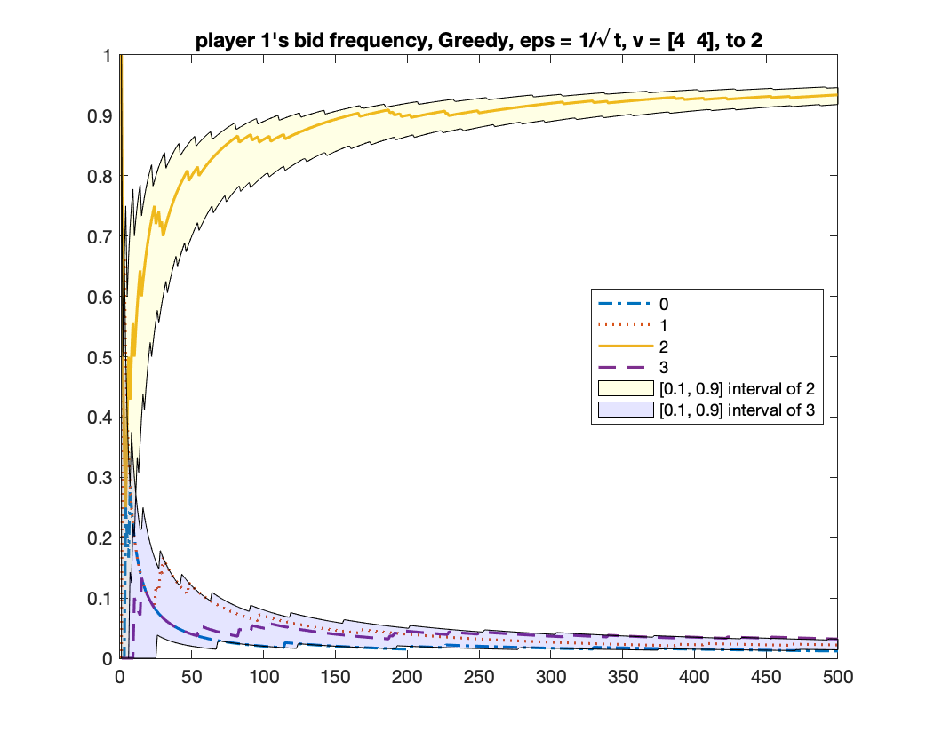
(a) Player 1’s bid frequency

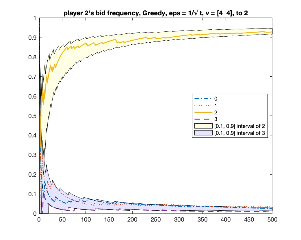
(b) Player 2’s bid frequency

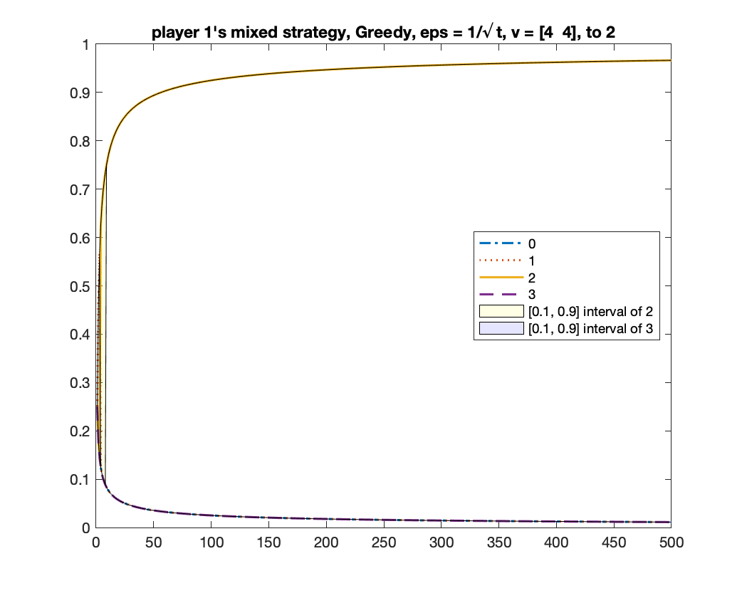
(c) Player 1’s mixed strategy

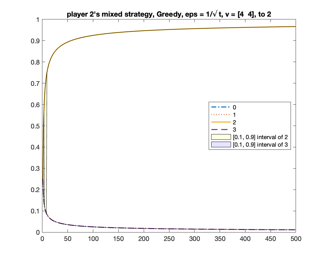
(d) Player 2’s mixed strategy

Figure 1: $|M^{1}|=2$, $\varepsilon_{t}$-Greedy, $v^{1}=v^{1}=4$, converging to $v^{1}-2=2$. The four curves in each plot show (a) (b) the changes of frequencies of bids $0,1,2,3$ and (c) (d) the changes of mixed strategies, in one simulation. The frequency of $2$ approaches $1$. The two regions show the $[10\%,90\%]$-confidence intervals of the corresponding curves (the upper is for bid $2$, the lower is for bid $3$), among all simulations that converge to $v^{1}-2$.

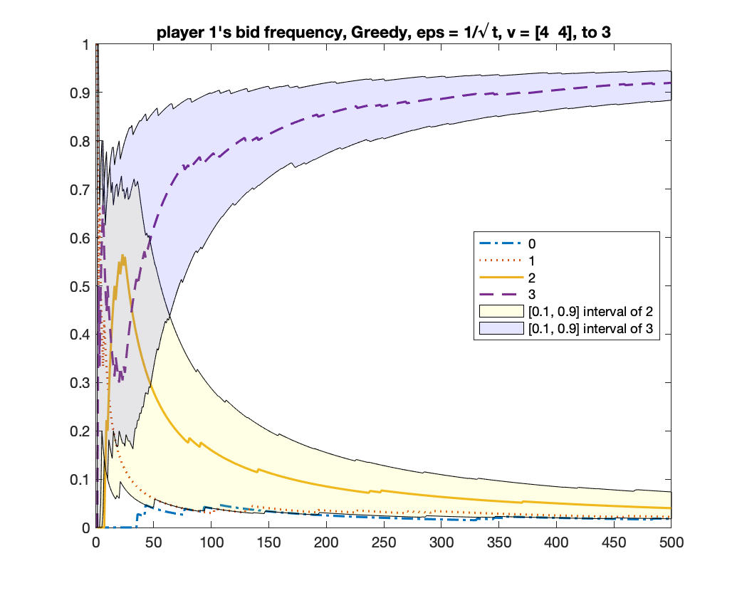
(a) Player 1’s bid frequency

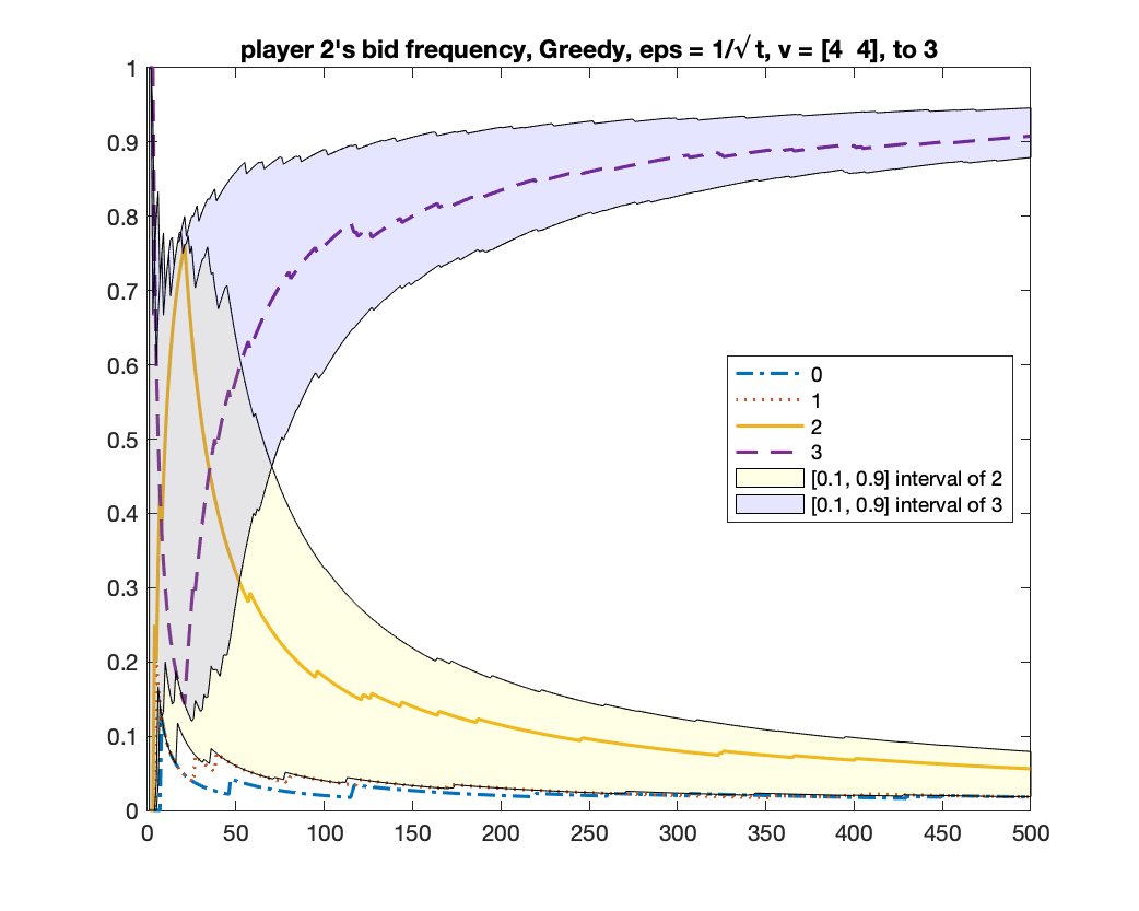
(b) Player 2’s bid frequency

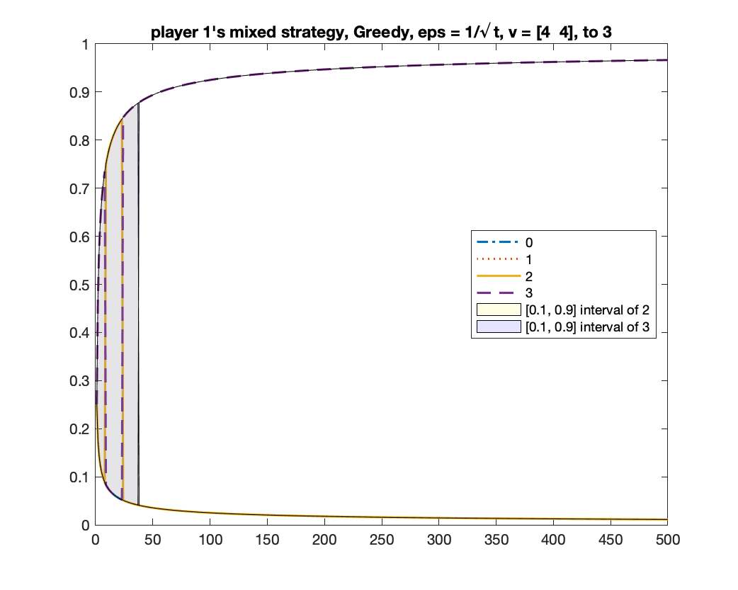
(c) Player 1’s mixed strategy

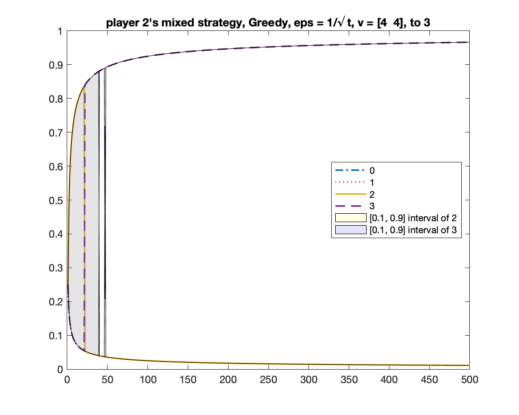
(d) Player 2’s mixed strategy

Figure 2: $|M^{1}|=2$, $\varepsilon_{t}$-Greedy, $v^{1}=v^{1}=4$, converging to $v^{1}-1=3$. The four curves in each plot show (a) (b) the changes of frequencies of bids $0,1,2,3$ and (c) (d) the changes of mixed strategies, in one simulation. The frequency of $3$ approaches $1$. The two regions show the $[10\%,90\%]$-confidence intervals of the corresponding curves (the upper is for bid $3$, the lower is for bid $2$), among all simulations that converge to $v^{1}-1$.

MWU always converges to $v^{1}-1$

We run MWU with $\varepsilon_{t}=\sqrt{1/t}$. Same as the previous experiment, we run the algorithm for $1000$ times and count how many times the algorithm converges to the equilibrium of $v^{1}-2$ and to $v^{1}-1$. We found that, in all $1000$ times, MWU converged to $v^{1}-1$. Figure 3 shows the changes of bid frequencies and mixed strategies of both players.

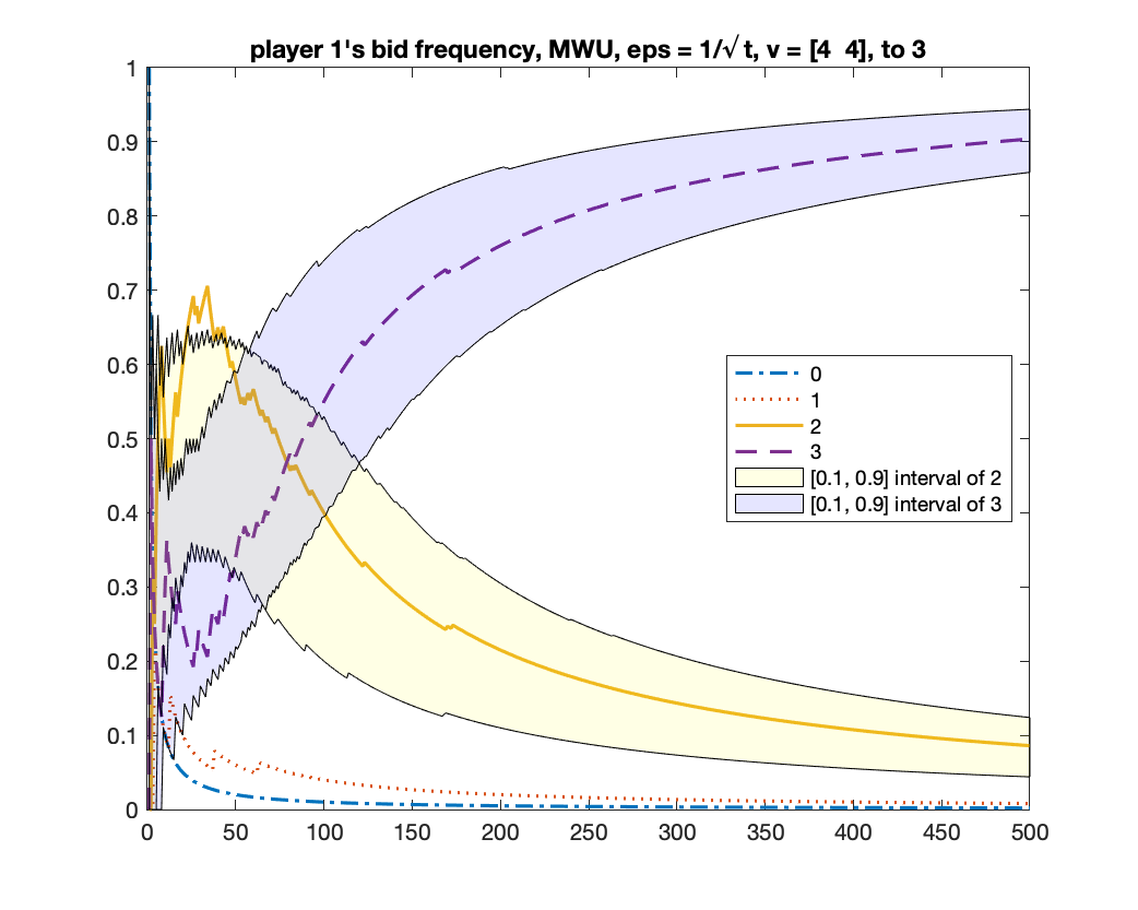
(a) Player 1’s bid frequency

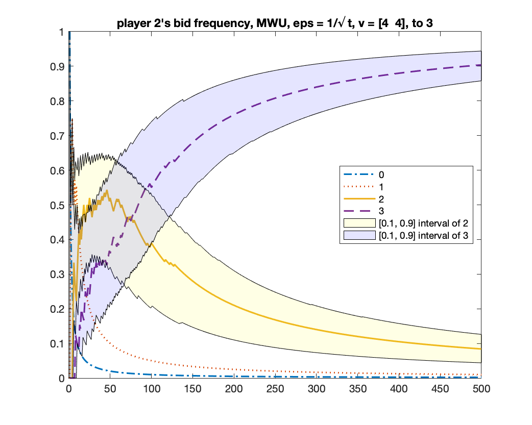
(b) Player 2’s bid frequency

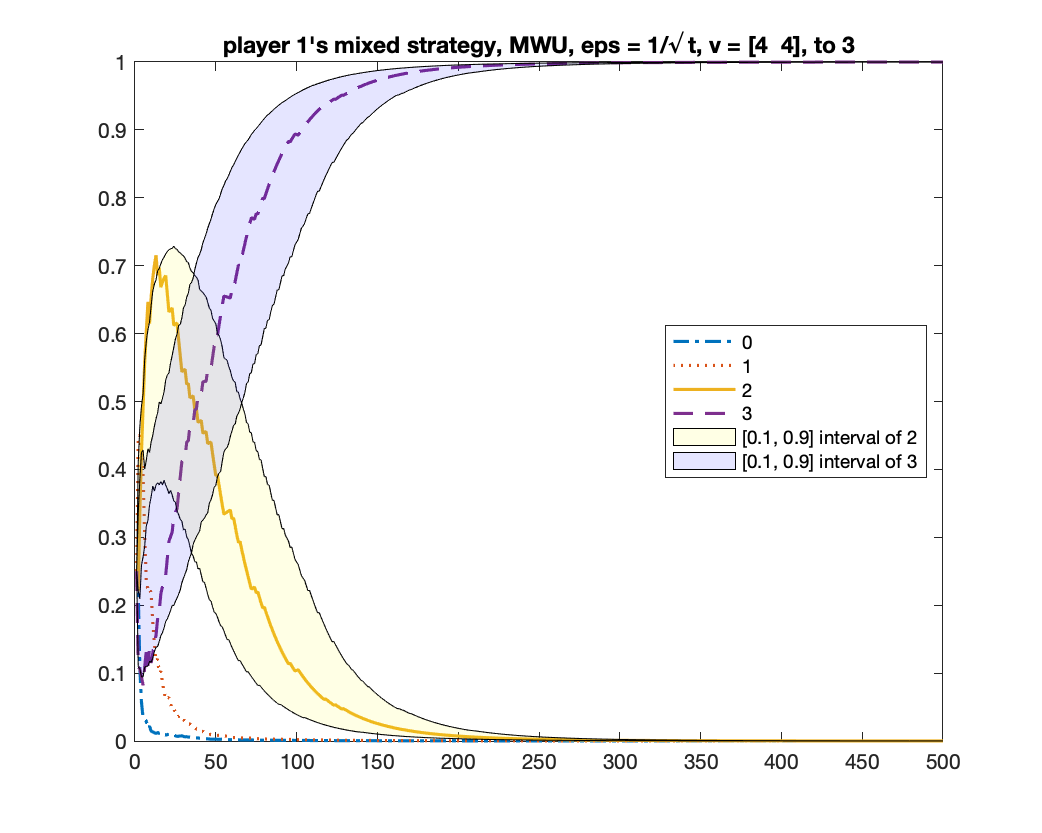
(c) Player 1’s mixed strategy

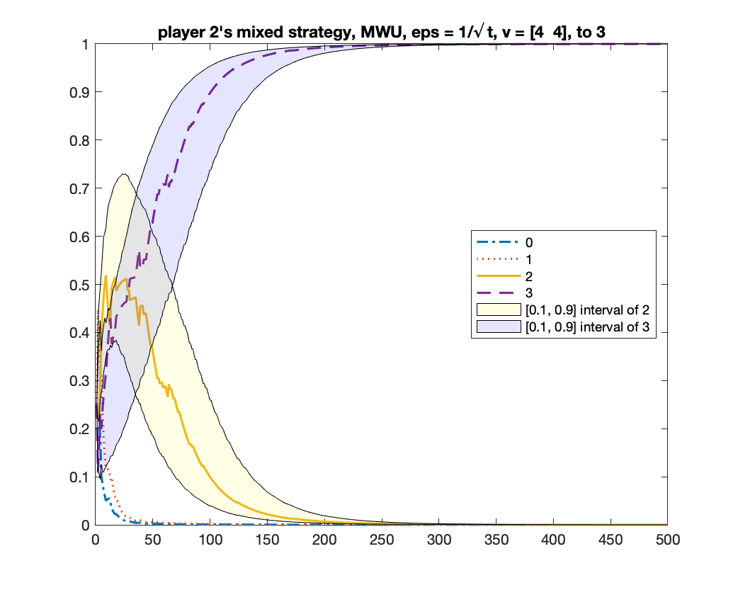
(d) Player 2’s mixed strategy

Figure 3: $|M^{1}|=2$, MWU, $v^{1}=v^{1}=4$, converging to $v^{1}-1=3$. The four curves in each plot show (a) (b) the changes of frequencies of bids $0,1,2,3$ and (c) (d) the changes of mixed strategies, in one simulation. The frequency of $3$ approaches $1$. The two regions show the $[10\%,90\%]$-confidence intervals of the corresponding curves (the upper is for bid $3$, the lower is for bid $2$), among 1000 simulations.

5.2 $|M^{1}|=1$: Non-Convergence

For the case of $|M^{1}|=1$ we showed that not all mean-based algorithms can converge to equilibrium, using the example of Follow the Leader (Example 7). Here we experimentally demonstrate that such non-convergence phenomena can also happen with more natural (and even no-regret) mean-based algorithms like $\varepsilon$-Greedy and MWU.

In the experiment we let $n=2$, $v^{1}=8,v^{2}=6$. We run $\varepsilon_{t}$-Greedy and MWU both with $\varepsilon_{t}=1/\sqrt{t}$ for $T=20000$ rounds.

For $\varepsilon_{t}$-Greedy, Figure 4 shows that the two bidders do not converge to a pure-strategy equilibrium, either in time-average or last-iterate. According to Proposition 3, a pure-strategy equilibrium must have bidder $1$ bidding $v^{2}=6$ and bidder $2$ bidding $v^{2}-1=5$. But figure (b) shows that bidder $2$’s frequency of bidding $5$ does not converge to $1$. The frequency oscillates and we do not know whether it will stabilize at some limit less than $1$. Looking closer, we see that bidder $2$ constantly switches between bids $5$ and $3$, and bidder $1$ switches between $5$ and $6$. Intuitively, this is because: in the $\varepsilon_{t}$-Greedy algorithm, when bidder $1$ bids $v^{2}=6$ with high probability, she also sometimes (with probability $\varepsilon_{t}$) chooses bids uniformly at random, in which case the best response for bidder $2$ is to bid $v^{2}/2=3$; but after bidder $2$ switches to $3$, bidder $1$ will find it beneficial to lower her bid from $6$ to $5$; then, bidder $2$ will switch to $5$ to compete with bidder $1$, winning the item with probability $1/2$; but then bidder $1$ will increase to $6$ to outbid bidder $2$; … In this way, they enter a cycle.

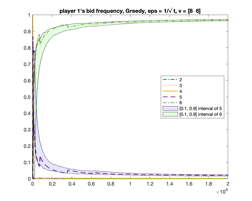
(a) Player 1’s bid frequency

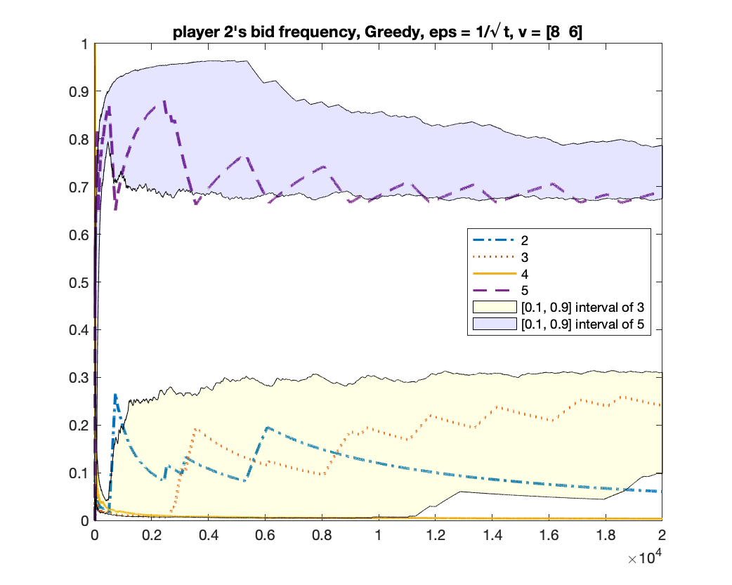
(b) Player 2’s bid frequency

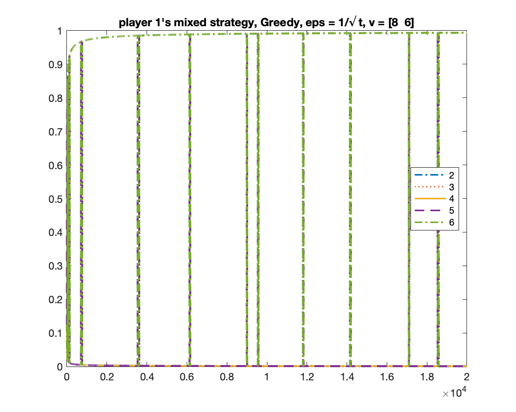
(c) Player 1’s mixed strategy

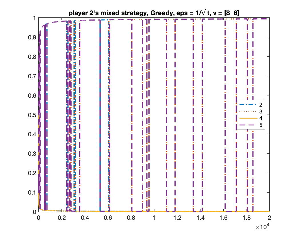
(d) Player 2’s mixed strategy

Figure 4: $|M^{1}|=1$, $\varepsilon_{t}$-Greedy, $v^{1}=8,v^{2}=6$. (a) Player 1’s frequency of bidding $v^{2}=6$ seems to converge to $1$. (b) Player 2’s bid frequency oscillates. (c) Player 1’s mixed strategy does not last-iterate converge; she switches between bids $5$ and $6$. (d) Player 2 switches between bids $3$ and $5$. The curves shown are results from one simulation. The region around the curves in (a) (b) are $[10\%,90\%]$-confidence intervals of the curves among 100 simulations.

For MWU, Figure 5 shows that: bidder 1’s bid frequency (a) and mixed strategy (c) seem to converge to bidding $v^{2}=6$; but bidder 2’s bid frequency (b) and mixed strategy (d) do not seem to converge.

(a) Player 1’s bid frequency

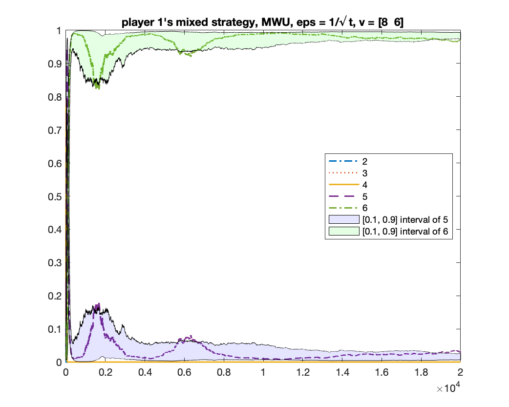
(b) Player 2’s bid frequency

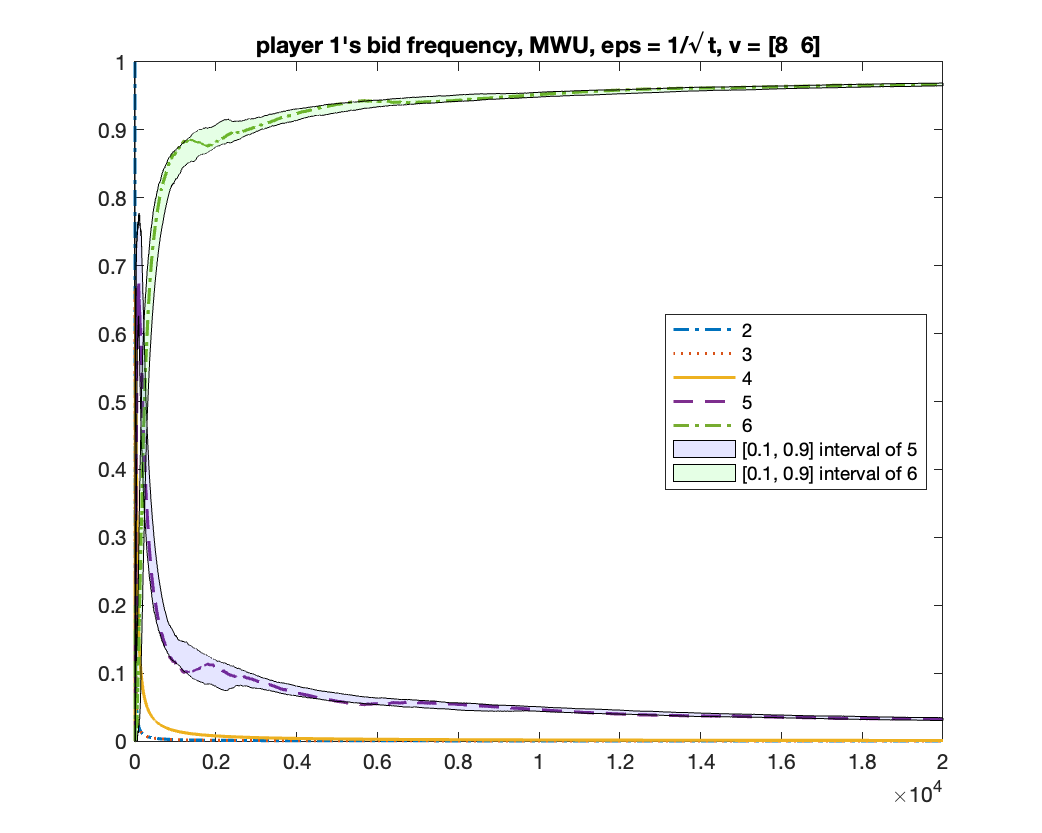
(c) Player 1’s mixed strategy

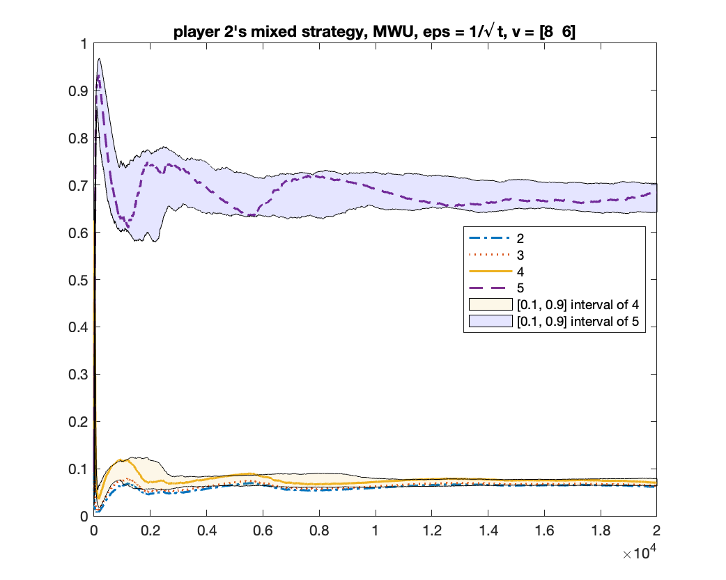
(d) Player 2’s mixed strategy

Figure 5: $|M^{1}|=1$, MWU, $v^{1}=8,v^{2}=6$. Player 1’s bid frequency (a) and mixed strategy (c) seem to converge to bidding $v^{2}=6$. But player 2’s bid frequency (b) and mixed strategy (d) do not seem to converge. The curves shown are results from one simulation. The region around the curves are $[10\%,90\%]$-confidence intervals of the curves among 100 simulations.

6 Conclusions and Future Directions

In this work we show that, in repeated fixed-value first price auctions, mean-based learning bidders converge to a Nash equilibrium in the presence of competition, in the sense that at least two bidders share the highest value. Without competition, we give non-convergence examples using mean-based algorithms that are not necessarily no-regret. Understanding the convergence property of no-regret algorithms in the absence of competition is a natural and interesting future direction. In fact, Kolumbus and Nisan, (2022) show that some non-mean-based no-regret algorithms do not converge. It is hence open to prove (non-)convergence for mean-based no-regret algorithms.

The convergence result we give is in the limit sense. As observed by Wu et al., (2022), many no-regret algorithms actually need an exponential time to converge to Nash equilibrium in some iterative-dominance-solvable game. Our theoretical analysis for the first price auction demonstrates a $T=O(c^{O(v^{1})})$ upper bound on the convergence time for the case of $|M^{1}|=3$. But the convergence time in our experiments is significantly shorter. The exact convergence rate remains open.

Analyzing repeated first price auctions where bidders have time-varying values is also a natural, yet possibly challenging, future direction.

Appendix A Missing Proofs from Section 3

A.1 Proof of Theorem 5

Suppose $|M^{1}|=2$. We will prove that, for any sufficiently large integer $T_{b}$, with probability at least $1-\exp\big{(}-\frac{T_{b}}{24NV}\big{)}-2\exp\big{(}-\frac{T_{b}}{1152N^{2}V^{2}}\big{)}-\frac{6}{e-2}\big{(}\frac{48NV}{T_{b}}\big{)}^{3e/4}$, one of following two events must happen:

• $\lim_{t\to\infty}\frac{1}{t}\sum_{s=1}^{t}\mathbb{I}[\forall i\in M^{1},b_{s}^{i}=v^{1}-2]=1$;

• $\lim_{t\to\infty}\frac{1}{t}\sum_{s=1}^{t}\mathbb{I}[\forall i\in M^{1},b_{s}^{i}=v^{1}-1]=1$ and $\lim_{t\to\infty}\Pr[b_{t}^{i}=v^{1}-1]=1$.

And if $n\geq 3$ and $v^{3}=v^{1}-1$, only the second event happens. Letting $T_{b}\to\infty$ proves Theorem 5.

We reuse the argument in Section 4.2. Assume $v^{1}\geq 3$. Recall that we defined $c=1+\frac{1}{12NV}$, $d=\lceil\log_{c}(8NV)\rceil$; $T_{b}$ is any integer such that $\gamma_{T_{b}}<\frac{1}{12N^{2}V^{2}}$ and $\exp\left(-\frac{(c-1)T_{b}}{1152N^{2}V^{2}}\right)\leq\frac{1}{2}$; $T_{0}=12NVT_{b}$; $T_{v^{1}-3}=c^{(v^{1}-3)d}T_{0}$. We defined $A_{v^{1}-3}$ to be the event $\frac{1}{T_{v^{1}-3}}\sum_{t=1}^{T_{v^{1}-3}}\mathbb{I}[\exists i\in M^{1},b_{t}^{i}\leq v^{1}-3]\leq\frac{1}{4NV}$. According to Corollary 13, $A_{v^{1}-3}$ holds with probability at least $1-\exp\left(-\frac{T_{b}}{24NV}\right)-2\exp\left(-\frac{T_{b}}{1152N^{2}V^{2}}\right)$. Suppose $A_{v^{1}-3}$ holds.

Now we partition the time horizon after $T_{v^{1}-3}$ as follows: let $T_{a}^{0}=T_{v^{1}-3},T_{a}^{k}=C(k+24NV)^{2}$, $\forall k\geq 0$, where $C=\frac{T_{v^{1}-3}}{(24NV)^{2}}$, so that $T_{a}^{0}=C(0+24NV)^{2}$. Denote $\Gamma_{a}^{k+1}=[T_{a}^{k}+1,T_{a}^{k+1}]$, with $|\Gamma_{a}^{k+1}|=T_{a}^{k+1}-T_{a}^{k}$. (We note that the notations here have different meanings than those in Section 4.3.) We define $\delta_{t}=(\frac{1}{t})^{1/8},t\geq 0$. For each $k\geq 0$, we define

$$F_{T_{a}^{k}}=\frac{T_{a}^{0}}{T_{a}^{k}}\frac{1}{4NV}+\sum_{s=0}^{k-1}\frac{T_{a}^{s+1}-T_{a}^{s}}{T_{a}^{k}}\delta_{T_{a}^{s}}+\sum_{s=0}^{k-1}\frac{T_{a}^{s+1}-T_{a}^{s}}{T_{a}^{k}}|M^{1}|V\gamma_{T_{a}^{s}}.$$

Let $A_{a}^{k}$ be event

$$A_{a}^{k}=\left[\frac{1}{T_{a}^{k}}\sum_{t=1}^{T_{a}^{k}}\mathbb{I}[\exists i\in M^{1},b_{t}^{i}\leq v^{1}-3]\leq F_{T_{a}^{k}}\right].$$

We note that $A_{a}^{0}=A_{v^{1}-3}$ because $F_{T_{a}^{0}}=\frac{1}{4NV}$.

In the proof we will always let $T_{b}$ to be sufficiently large. This implies that all the times $T_{0},T_{v^{1}-3},T_{a}^{0},T_{a}^{k}$, etc., are sufficiently large.

A.1.1 Additional Notations, Claims, and Lemmas

Claim 16.

When $T_{b}$ is sufficiently large,

• $F_{T_{a}^{k+1}}\leq F_{T_{a}^{k}}\leq\frac{1}{4NV}$ for every $k\geq 0$.

• $\lim_{k\to\infty}F_{T_{a}^{k}}=0$.

Proof.

Since $\delta_{T_{a}^{0}}\to 0$ and $\gamma_{T_{a}^{0}}\to 0$ as $T_{b}\to\infty$, when $T_{b}$ is sufficiently large we have

$$F_{T_{a}^{1}}=\frac{T_{a}^{0}}{T_{a}^{1}}\frac{1}{4NV}+\frac{T_{a}^{1}-T_{a}^{0}}{T_{a}^{1}}\left(\delta_{T_{a}^{0}}+|M^{1}|V\gamma_{T_{a}^{0}}\right)\leq\frac{T_{a}^{0}}{T_{a}^{1}}\frac{1}{4NV}+\frac{T_{a}^{1}-T_{a}^{0}}{T_{a}^{1}}\frac{1}{4NV}=\frac{1}{4NV}=F_{T_{a}^{0}}.$$

Since $\delta_{T_{a}^{s}}$ and $\gamma_{T_{a}^{s}}$ are both decreasing, we have

$$F_{T_{a}^{k}} >\sum_{s=0}^{k-1}\frac{T_{a}^{s+1}-T_{a}^{s}}{T_{a}^{k}}\delta_{T_{a}^{s}}+\sum_{s=0}^{k-1}\frac{T_{a}^{s+1}-T_{a}^{s}}{T_{a}^{k}}|M^{1}|V\gamma_{T_{a}^{s}}$$

$$\geq\sum_{s=0}^{k-1}\frac{T_{a}^{s+1}-T_{a}^{s}}{T_{a}^{k}}\delta_{T_{a}^{k}}+\sum_{s=0}^{k-1}\frac{T_{a}^{s+1}-T_{a}^{s}}{T_{a}^{k}}|M^{1}|V\gamma_{T_{a}^{k}}~{}=~{}\delta_{T_{a}^{k}}+|M^{1}|V\gamma_{T_{a}^{k}}.$$

Thus,

$$F_{T_{a}^{k+1}} \stackrel{{\scriptstyle\text{by definition}}}{{=}}\frac{T_{a}^{k}}{T_{a}^{k+1}}F_{T_{a}^{k}}+\frac{T_{a}^{k+1}-T_{a}^{k}}{T_{a}^{k+1}}\left(\delta_{T_{a}^{k}}+|M^{1}|V\gamma_{T_{a}^{k}}\right)<\frac{T_{a}^{k}}{T_{a}^{k+1}}F_{T_{a}^{k}}+\frac{T_{a}^{k+1}-T_{a}^{k}}{T_{a}^{k+1}}F_{T_{a}^{k}}=F_{T_{a}^{k}}.$$

Then we prove $\lim_{k\to\infty}F_{T_{a}^{k}}=0$. For every $0<\varepsilon<\frac{1}{4NV}$, we can find $k$ sufficiently large such that $\delta_{T_{a}^{k}}\leq\frac{\varepsilon}{6}$, and $\gamma_{T_{a}^{k}}\leq\frac{\varepsilon}{6|M^{1}|V}$. For any $l\geq\lceil k/\varepsilon\rceil$, we have $\frac{T_{a}^{0}}{T_{a}^{l}}\leq\frac{T_{a}^{k}}{T_{a}^{l}}\leq\frac{\varepsilon}{6}$. Then

$$F_{T_{a}^{l}} =\frac{T_{a}^{0}}{T_{a}^{l}}\frac{1}{4NV}+\sum_{s=0}^{l-1}\frac{T_{a}^{s+1}-T_{a}^{s}}{T_{a}^{l}}(\delta_{T_{a}^{s}}+|M^{1}|V\gamma_{T_{a}^{s}})$$

$$\leq\frac{\varepsilon}{3}+2\sum_{s=0}^{k-1}\frac{T_{a}^{s+1}-T_{a}^{s}}{T_{a}^{l}}+\sum_{s=k}^{l-1}\frac{T_{a}^{s+1}-T_{a}^{s}}{T_{a}^{l}}(\delta_{T_{a}^{k}}+|M^{1}|V\gamma_{T_{a}^{k}})$$

$$\leq\frac{\varepsilon}{3}+2\frac{T_{a}^{k}}{T_{a}^{l}}+\delta_{T_{a}^{k}}+|M^{1}|V\gamma_{T_{a}^{k}}$$

$$\leq\frac{\varepsilon}{3}+\frac{\varepsilon}{3}+\frac{\varepsilon}{3}=\varepsilon.$$

Since $F_{T_{a}^{k}}$ is non-negative, we have $\lim_{k\to\infty}F_{T_{a}^{k}}=0$. ∎

Claim 17.

$\sum_{s=0}^{\infty}\exp\left(-\frac{1}{2}|\Gamma_{a}^{s+1}|\delta_{T_{a}^{s}}^{2}\right)\leq\frac{2}{e-2}\frac{1}{C^{3e/4}}\leq\frac{2}{e-2}\big{(}\frac{48NV}{T_{b}}\big{)}^{3e/4}$.

Proof.

Recall that $|\Gamma_{a}^{s+1}|=T_{a}^{s+1}-T_{a}^{s}$, $\delta_{T_{a}^{s}}^{2}=(\frac{1}{T_{a}^{s}})^{1/8}$, and $T_{a}^{s}=C(s+24NV)^{2}$. Hence,

$$\sum_{s=0}^{\infty}\exp\left(-\frac{1}{2}|\Gamma_{a}^{s+1}|\delta_{T_{a}^{s}}^{2}\right) =\sum_{s=0}^{\infty}\exp\left(-\frac{1}{2}\big{(}T_{a}^{s+1}-T_{a}^{s}\big{)}\big{(}\frac{1}{T_{a}^{s}}\big{)}^{1/4}\right)$$

$$=\sum_{s=0}^{\infty}\exp\left(-\frac{1}{2}C\big{(}2(s+24NV)+1\big{)}\big{(}\frac{1}{C(s+24NV)^{2}}\big{)}^{1/4}\right)$$

$$\leq\sum_{s=0}^{\infty}\exp\left(-C^{3/4}\big{(}s+24NV\big{)}\big{(}\frac{1}{s+24NV}\big{)}^{1/2}\right)$$

$$=\sum_{s=0}^{\infty}\exp\left(-C^{3/4}\sqrt{s+24NV}\right)$$

$$\leq\sum_{x=2}^{\infty}\exp\left(-C^{3/4}\sqrt{x}\right)$$

$$\leq\int_{x=1}^{\infty}\exp\left(-C^{3/4}\sqrt{x}\right)\mathrm{d}x$$

(using $$e^{x}\geq x^{e} x\geq 0 \leq\int_{x=1}^{\infty}\frac{1}{(C^{3/4}\sqrt{x})^{e}}\mathrm{d}x=\frac{1}{C^{3e/4}}\cdot\frac{2}{e-2}.$$ for )

Substituting $C=\frac{T_{v^{1}-3}}{(24NV)^{2}}=\frac{c^{(v^{1}-3)d}12NVT_{b}}{(24NV)^{2}}\geq\frac{12NVT_{b}}{(24NV)^{2}}=\frac{T_{b}}{48NV}$ proves the claim. ∎

Fact 18.

$\frac{T_{a}^{k}}{T_{a}^{k+1}}\geq 1-\frac{2}{k+24NV}$.

Proof.

By definition,

$$\frac{T_{a}^{k}}{T_{a}^{k+1}}=\frac{(k+24NV)^{2}}{(k+24NV+1)^{2}}=1-\frac{2(k+24NV)+1}{(k+24NV+1)^{2}}\geq 1-\frac{2}{k+24NV+1}\geq 1-\frac{2}{k+24NV}.$$

∎

Claim 19.

When $A_{a}^{k}$ holds, we have, for every $t\in\Gamma_{a}^{k+1}=[T_{a}^{k}+1,T_{a}^{k+1}]$,

$$\frac{1}{t-1}\sum_{s=1}^{t-1}\mathbb{I}[\exists i\in M^{1},b_{s}^{i}\leq v^{1}-3]\leq F_{T_{a}^{k}}+\frac{2}{k+24NV}\leq\frac{1}{2NV}-2\gamma_{t}.$$

Proof.

When $A_{a}^{k}$ holds, for every $t\in\Gamma_{a}^{k+1}$,

$$\frac{1}{t-1}\sum_{s=1}^{t-1}\mathbb{I}[\exists i\in M^{1},b_{s}^{i}\leq v^{1}-3] \leq\frac{1}{t-1}\left(T_{a}^{k}F_{T_{a}^{k}}+(t-1-T_{a}^{k})\right)$$

(since $$T_{a}^{k}\leq t-1\leq T_{a}^{k+1} \leq F_{T_{a}^{k}}+\frac{T_{a}^{k+1}-T_{a}^{k}}{T_{a}^{k+1}}$$)

(by Fact 18) $$\leq F_{T_{a}^{k}}+\frac{2}{k+24NV}.$$

Since $F_{T_{a}^{k}}\leq\frac{1}{4NV}$ by Claim 16 and $\gamma_{t}\leq\frac{1}{12N^{2}V^{2}}$ by assumption, the above expression is further bounded by $\frac{1}{4NV}+\frac{2}{k+24NV}\leq\frac{1}{4NV}+\frac{2}{24NV}=\frac{1}{3NV}\leq\frac{1}{2NV}-2\gamma_{t}$. ∎

Lemma 20.

For every $k\geq 0$, $\Pr[A_{a}^{k+1}\mid A_{a}^{k}]\geq 1-\exp\left(-\frac{1}{2}|\Gamma_{a}^{k+1}|\delta_{T_{a}^{k}}^{2}\right)$.

Proof.

Given $A_{a}^{k}$, according to Claim 19, it holds that for every $t\in\Gamma_{a}^{k+1}$, $\frac{1}{t-1}\sum_{s=1}^{t-1}\mathbb{I}[\exists i\in M^{1},b_{s}^{i}\leq v^{1}-3]\leq\frac{1}{2NV}-2\gamma_{t}$. Then according to Claim 8, for any history $H_{t-1}$,

$$\Pr[\exists i\in M^{1},b_{t}^{i}\leq v^{1}-3\mid H_{t-1},A_{a}^{k}]\leq|M^{1}|V\gamma_{t}.$$

Let $Z_{t}=\mathbb{I}[\exists i\in M^{1},b_{t}^{i}\leq v^{1}-3]-|M^{1}|V\gamma_{t}$ and let $X_{t}=\sum_{s=T_{a}^{k}+1}^{t}Z_{s}$. We have ${\mathbb{E}}{\mathchoice{\left[Z_{t}\mid H_{t-1},A_{a}^{k}\right]}{[Z_{t}\mid H_{t-1},A_{a}^{k}]}{[Z_{t}\mid H_{t-1},A_{a}^{k}]}{[Z_{t}\mid H_{t-1},A_{a}^{k}]}}\leq 0$. Therefore, the sequence $X_{T_{a}^{k}+1},X_{T_{a}^{k}+2},\ldots,X_{T_{a}^{k+1}}$ is a supermartingale (with respect to the sequence of history $H_{T_{a}^{k}},H_{T_{a}^{k}+1},\ldots,H_{T_{a}^{k+1}-1}$). By Azuma’s inequality, for any $\Delta>0$, we have

$$\Pr\Bigg{[}\sum_{t\in\Gamma_{a}^{k+1}}Z_{t}\geq\Delta\;\bigg{|}\;A_{a}^{k}\Bigg{]}\leq\exp\left(-\frac{\Delta^{2}}{2|\Gamma_{a}^{k+1}|}\right).$$

Let $\Delta=|\Gamma_{a}^{k+1}|\delta_{T_{a}^{k}}$. Then with probability at least $1-\exp\big{(}-\frac{1}{2}|\Gamma_{a}^{k+1}|\delta_{T_{a}^{k}}^{2}\big{)}$, we get $\sum_{t\in\Gamma_{a}^{k+1}}\mathbb{I}[\exists i\in M^{1},b_{t}^{i}\leq v^{1}-3]\;<\;\Delta+|M^{1}|V\sum_{t\in\Gamma_{a}^{k+1}}\gamma_{t}\;\leq\;|\Gamma_{a}^{k+1}|\delta_{T_{a}^{k}}+|M^{1}|V|\Gamma_{a}^{k+1}|\gamma_{T_{a}^{k}}$, which implies

$$\frac{1}{T_{a}^{k+1}}\sum_{t=1}^{T_{a}^{k+1}}\mathbb{I}[\exists i\in M^{1},b_{t}^{i}\leq v^{1}-3]$$

$$=\frac{1}{T_{a}^{k+1}}\bigg{(}\sum_{t=1}^{T_{a}^{k}}\mathbb{I}[\exists i\in M^{1},b_{t}^{i}\leq v^{1}-3]+\sum_{t\in\Gamma_{a}^{k+1}}\mathbb{I}[\exists i\in M^{1},b_{t}^{i}\leq v^{1}-3]\bigg{)}$$

$$\leq\frac{1}{T_{a}^{k+1}}\left(T_{a}^{k}F_{T_{a}^{k}}+|\Gamma_{a}^{k+1}|\delta_{T_{a}^{k}}+|M^{1}|V|\Gamma_{a}^{k+1}|\gamma_{T_{a}^{k}}\right)$$

(by definition) $$=F_{T_{a}^{k+1}}$$

and thus $A_{a}^{k+1}$ holds. ∎

Denote by $f_{t}^{i}(b)$ the frequency of bid $b$ in the first $t$ rounds for bidder $i$:

$$f_{t}^{i}(b)=\frac{1}{t}\sum_{s=1}^{t}\mathbb{I}[b_{s}^{i}=b].$$

Let $f_{t}^{i}(0:v^{1}-3)=\frac{1}{t}\sum_{s=1}^{t}\mathbb{I}[b_{s}^{i}\leq v^{1}-3]$.

Claim 21.

If the history $H_{t-1}$ satisfies $f_{t-1}^{i}(v^{1}-1)>2(X+V\gamma_{t})$ and $\frac{1}{t-1}\sum_{s=1}^{t-1}\mathbb{I}[\exists i\in M^{1},b_{s}^{i}\leq v^{1}-3]\leq X$ for some $X\in[0,1]$, then we have $\Pr[b_{t}^{i^{\prime}}=v^{1}-2\mid H_{t-1}]\leq\gamma_{t}$ for the other $i^{\prime}\neq i\in M^{1}$.

Proof.

Consider $\alpha_{t-1}^{i^{\prime}}(v^{1}-1)$ and $\alpha_{t-1}^{i^{\prime}}(v^{1}-2)$. On the one hand,

$$\alpha_{t-1}^{i^{\prime}}(v^{1}-1)=1\times(1-f_{t-1}^{i}(v^{1}-1))+\frac{1}{2}\times f_{t-1}^{i}(v^{1}-1)=1-\frac{1}{2}f_{t-1}^{i}(v^{1}-1).$$ (7)

On the other hand, since having more bidders with bids no larger than $v^{1}-2$ only decreases the utility of a bidder who bids $v^{1}-2$, we can upper bound $\alpha_{t-1}^{i^{\prime}}(v^{1}-2)$ by

$$\alpha_{t-1}^{i^{\prime}}(v^{1}-2) \leq 2\times f_{t-1}^{i}(0:v^{1}-3)+1\times(1-f_{t-1}^{i}(v^{1}-1)-f_{t-1}^{i}(0:v^{1}-3))$$

$$=1-f_{t-1}^{i}(v^{1}-1)+f_{t-1}^{i}(0:v^{1}-3)$$

$$\leq 1-f_{t-1}^{i}(v^{1}-1)+X,$$ (8)

where the last inequality holds because $f_{t-1}^{i}(0:v^{1}-3)\leq\frac{1}{t-1}\sum_{s=1}^{t-1}\mathbb{I}[\exists i\in M^{1},b_{s}^{i}\leq v^{1}-3]\leq X$. Combining $(\ref{eq:v^1-1})$ and $(\ref{eq:v^1-2})$, we get

$$\alpha_{t-1}^{i^{\prime}}(v^{1}-1)-\alpha_{t-1}^{i^{\prime}}(v^{1}-2)\geq(1-\frac{1}{2}f_{t-1}^{i})-(1-f_{t-1}^{i}+X)=\frac{1}{2}f_{t-1}^{i}(v^{1}-1)-X>V\gamma_{t}.$$

This implies $\Pr[b_{t}^{i^{\prime}}=v^{1}-2\mid H_{t-1}]\leq\gamma_{t}$ according to the mean-based property. ∎

A.1.2 Proof of the General Case

We consider $k=0,1,\ldots$ to $\infty$. For each $k$, we suppose $A_{a}^{0},A_{a}^{1},\ldots,A_{a}^{k}$ hold, which happens with probability at least $1-\sum_{s=0}^{k-1}\exp\big{(}-\frac{1}{2}|\Gamma_{a}^{s+1}|\delta_{T_{a}^{s}}^{2}\big{)}$ according to Lemma 20, given that $A_{a}^{0}=A_{v^{1}-3}$ already held. The proof is divided into two cases based on $f_{T_{a}^{k}}^{i}(v^{1}-1)$.

Case 1:

For all $k\geq 0$, $f_{T_{a}^{k}}^{i}(v^{1}-1)\leq 16(F_{T_{a}^{k}}+\frac{2}{k+24NV}+V\gamma_{T_{a}^{k}})$ for both $i\in M^{1}$.

We argue that the two bidders in $M^{1}$ converge to playing $v^{1}-2$ in this case.

According to Lemma 20, all events $A_{a}^{0},A_{a}^{1},\ldots,A_{a}^{k},\ldots$ happen with probability at least $1-\sum_{k=0}^{\infty}\exp\left(-\frac{1}{2}|\Gamma_{a}^{k+1}|\delta_{T_{a}^{k}}^{2}\right)$. Claim 19 and Claim 16 then imply that, for both $i\in M^{1}$,

$$\lim_{t\to\infty}f_{t}^{i}(0:v^{1}-3)\leq\lim_{k\to\infty}\left(F_{T_{a}^{k}}+\frac{2}{k+24NV}\right)=0.$$

Because for every $t\in\Gamma_{a}^{k+1}=[T_{a}^{k}+1,T_{a}^{k+1}]$ we have $f_{t}^{i}(v^{1}-1)\leq\frac{T_{a}^{k+1}}{t}f_{T_{a}^{k}}^{i}(v^{1}-1)\leq\frac{T_{a}^{k+1}}{T_{a}^{k}}f_{T_{a}^{k}}^{i}(v^{1}-1)\leq 2f_{T_{a}^{k}}^{i}(v^{1}-1)$ and by condition $f_{T_{a}^{k}}^{i}(v^{1}-1)\to 0$ as $k\to\infty$, we have

$$\lim_{t\to\infty}f_{t}^{i}(v^{1}-1)=0.$$

Therefore,

$$\lim_{t\to\infty}f_{t}^{i}(v^{1}-2)=\lim_{t\to\infty}1-f_{t}^{i}(0:v^{1}-3)-f_{t}^{i}(v^{1}-1)=1,$$

which implies

$$\lim_{t\to\infty}\frac{1}{t}\sum_{s=1}^{t}\mathbb{I}[\forall i\in M^{1},b_{s}^{i}=v^{1}-2]=1.$$

Case 2:

There exists $k\geq 0$ such that $f_{T_{a}^{k}}^{i}(v^{1}-1)>16(F_{T_{a}^{k}}+\frac{2}{k+24NV}+V\gamma_{T_{a}^{k}})$ for some $i\in M^{1}$.

If this case happens, we argue that the two bidders in $M^{1}$ converge to playing $v^{1}-1$.

We first prove that, after $\ell=k+24NV$ periods (i.e., at time $T_{a}^{k+\ell}$), the frequency of $v^{1}-1$ for both bidders in $M^{1}$ is greater than $4(F_{T_{a}^{k+\ell}}+\frac{2}{(k+\ell)+24NV}+V\gamma_{T_{a}^{k+\ell}})$, with high probability.

Lemma 22.

Suppose that, at time $T_{a}^{k}$, $A_{a}^{k}$ holds and for some $i\in M^{1}$, $f_{T_{a}^{k}}^{i}(v^{1}-1)>16(F_{T_{a}^{k}}+\frac{2}{k+24NV}+V\gamma_{T_{a}^{k}})$ holds. Then, with probability at least $1-2\sum_{j=k}^{k+\ell-1}\exp\left(-\frac{1}{2}|\Gamma_{a}^{j+1}|\delta_{T_{a}^{j}}^{2}\right)$, the following events happen at time $T_{a}^{k+\ell}$, where $\ell=k+24NV$:

• $A_{a}^{k+\ell}$;

• For both $i\in M^{1}$, $f_{T_{a}^{k+\ell}}^{i}(v^{1}-1)>4(F_{T_{a}^{k+\ell}}+\frac{2}{(k+\ell)+24NV}+V\gamma_{T_{a}^{k+\ell}})$.

Proof.

We prove by an induction from $j=k$ to $k+\ell-1$. Given $A_{a}^{j}$, $A_{a}^{j+1}$ happens with probability at least $1-\exp\left(-\frac{1}{2}|\Gamma_{a}^{j+1}|\delta_{T_{a}^{j}}^{2}\right)$ according to Lemma 20. Hence, with probability at least $1-\sum_{j=k}^{k+\ell-1}\exp\left(-\frac{1}{2}|\Gamma_{a}^{j+1}|\delta_{T_{a}^{j}}^{2}\right)$, all events $A_{a}^{k},A_{a}^{k+1},\ldots,A_{a}^{k+\ell}$ happen.

Now we consider the second event. For all $t\in\Gamma_{a}^{j+1}$, noticing that $\frac{T_{a}^{k}}{t-1}\geq\frac{T_{a}^{k}}{T_{a}^{j+1}}\geq\frac{T_{a}^{k}}{T_{a}^{k+\ell}}=\frac{(k+24NV)^{2}}{(2(k+24NV))^{2}}=\frac{1}{4}$, we have

$$f_{t-1}^{i}(v^{1}-1)\geq\frac{T_{a}^{k}}{t-1}f_{T_{a}^{k}}^{i}(v^{1}-1) \geq\frac{1}{4}f_{T_{a}^{k}}^{i}(v^{1}-1)$$

(by condition) $$>4(F_{T_{a}^{k}}+\frac{2}{k+24NV}+V\gamma_{T_{a}^{k}})$$ (9)

($$F_{T_{a}^{k}} \gamma_{T_{a}^{k}} k \geq 4(F_{T_{a}^{j}}+\frac{2}{j+24NV}+V\gamma_{T_{a}^{j}}).$$ and are decreasing in )

According to Claim 19, given $A_{a}^{j}$ we have $\frac{1}{t-1}\sum_{s=1}^{t-1}\mathbb{I}[\exists i\in M^{1},b_{s}^{i}\leq v^{1}-3]\leq F_{T_{a}^{j}}+\frac{2}{j+24NV}\leq\frac{1}{2NV}-2\gamma_{t}$. Using Claim 21 with $X=F_{T_{a}^{j}}+\frac{2}{j+24NV}$, we have, for bidder $i^{\prime}\neq i,i^{\prime}\in M^{1}$, $\Pr[b_{t}^{i^{\prime}}=v^{1}-2\mid H_{t-1}]\leq\gamma_{t}$. By Claim 8, $\Pr[b_{t}^{i^{\prime}}\leq v^{1}-3\mid H_{t-1}]\leq(V-1)\gamma_{t}$. Combining the two, we get

$$\Pr[b_{t}^{i^{\prime}}=v^{1}-1\mid H_{t-1}]\geq 1-V\gamma_{t}.$$

Let $\Delta=|\Gamma_{a}^{k+1}|\delta_{T_{a}^{k}}$. Similar to the proof of Lemma 20, we can use Azuma’s inequality to argue that, with probability at least $1-\exp(-\frac{1}{2}|\Gamma_{a}^{k+1}|\delta_{T_{a}^{k}}^{2})$, it holds that

$$\sum_{t\in\Gamma_{a}^{j+1}}\mathbb{I}[b_{t}^{i^{\prime}}=v^{1}-1]\geq\sum_{t\in\Gamma_{a}^{j+1}}(1-V\gamma_{t}-\delta_{T_{a}^{j}})\geq|\Gamma_{a}^{j+1}|(1-V\gamma_{T_{a}^{j}}-\delta_{T_{a}^{j}}).$$

An induction shows that, with probability at least $1-\sum_{j=k}^{k+\ell-1}\exp\left(-\frac{1}{2}|\Gamma_{a}^{j+1}|\delta_{T_{a}^{j}}^{2}\right)$, $\sum_{t\in\Gamma_{a}^{j+1}}\mathbb{I}[b_{t}^{i^{\prime}}=v^{1}-1]\geq|\Gamma_{a}^{j+1}|(1-V\gamma_{T_{a}^{j}}-\delta_{T_{a}^{j}})$ holds for all $j\in\{k,\ldots,k+\ell-1\}$. Therefore,

$$f_{T_{a}^{k+\ell}}^{i^{\prime}}(v^{1}-1) \geq\frac{1}{T_{a}^{k+\ell}}\left(0+\sum_{t\in\Gamma_{a}^{k+1}\cup\cdots\cup\Gamma_{a}^{k+\ell}}\mathbb{I}[b_{t}^{i^{\prime}}=v^{1}-1]\right)$$

$$\geq\frac{1}{T_{a}^{k+\ell}}\left(|\Gamma_{a}^{k+1}|(1-V\gamma_{T_{a}^{k}}-\delta_{T_{a}^{k}})+\cdots+|\Gamma_{a}^{k+\ell}|(1-V\gamma_{T_{a}^{k+\ell-1}}-\delta_{T_{a}^{k+\ell-1}})\right)$$

$$\geq\frac{1}{T_{a}^{k+\ell}}\left((|\Gamma_{a}^{k+1}|+\cdots+|\Gamma_{a}^{k+\ell}|)\cdot(1-V\gamma_{T_{a}^{k}}-\delta_{T_{a}^{k}})\right)$$

$$=\frac{T_{a}^{k+\ell}-T_{a}^{k}}{T_{a}^{k+\ell}}(1-V\gamma_{T_{a}^{k}}-\delta_{T_{a}^{k}})$$

$$=\frac{4(k+24NV)^{2}-(k+24NV)^{2}}{4(k+24NV)^{2}}(1-V\gamma_{T_{a}^{k}}-\delta_{T_{a}^{k}})$$

$$=\frac{3}{4}(1-V\gamma_{T_{a}^{k}}-\delta_{T_{a}^{k}})$$

$$\stackrel{{\scriptstyle\text{(assuming $T_{b}$ is large enough) }}}{{>}}4\left(F_{T_{a}^{k+\ell}}+\frac{2}{(k+\ell)+24NV}+V\gamma_{T_{a}^{k+\ell}}\right).$$

This proves the claim for $i^{\prime}\in M^{1}$. The claim for $i\in M^{1}$ follows from (9) and the fact that $F_{T_{a}^{k}}$ and $\gamma_{T_{a}^{k}}$ are decreasing in $k$. ∎

We denote by $k_{0}=k+\ell$ the time period at which $f_{T_{a}^{k_{0}}}^{i}(v^{1}-1)>4(F_{T_{a}^{k_{0}}}+\frac{2}{k_{0}+24NV}+V\gamma_{T_{a}^{k_{0}}})$ for both $i\in M^{1}$. We continuing the analysis for each period $k\geq k_{0}$. Define sequence $(G_{T_{a}^{k}})$:

$$G_{T_{a}^{k}}=\frac{T_{a}^{k_{0}}}{T_{a}^{k}}\cdot 4\left(F_{T_{a}^{k_{0}}}+\frac{2}{k_{0}+24NV}+V\gamma_{T_{a}^{k_{0}}}\right)+\sum_{s=k_{0}}^{k-1}\frac{T_{a}^{s+1}-T_{a}^{s}}{T_{a}^{k}}(1-V\gamma_{T_{a}^{s}}-\delta_{T_{a}^{s}}),~{}\text{ for }k\geq k_{0},$$

where we recall that $\delta_{t}=(\frac{1}{t})^{1/8}$. We note that $f_{T_{a}^{k_{0}}}^{i}(v^{1}-1)>G_{T_{a}^{k_{0}}}=4\big{(}F_{T_{a}^{k_{0}}}+\frac{2}{k_{0}+24NV}+V\gamma_{T_{a}^{k_{0}}}\big{)}$.

Claim 23.

When $T_{b}$ is sufficiently large,

• $G_{T_{a}^{k}}\geq 4\big{(}F_{T_{a}^{k_{0}}}+\frac{2}{k_{0}+24NV}+V\gamma_{T_{a}^{k_{0}}}\big{)}$ for every $k\geq k_{0}$.

• $\lim_{k\to\infty}G_{T_{a}^{k}}=1$.

Proof.

Since $1-V\gamma_{T_{a}^{s}}-\delta_{T_{a}^{s}}\to 1$ as $T_{b}\to\infty$, for sufficiently large $T_{b}$ we have $1-V\gamma_{T_{a}^{s}}-\delta_{T_{a}^{s}}\geq 4\big{(}F_{T_{a}^{k_{0}}}+\frac{2}{k_{0}+24NV}+V\gamma_{T_{a}^{k_{0}}}\big{)}$ and hence $G_{T_{a}^{k}}\geq 4\big{(}F_{T_{a}^{k_{0}}}+\frac{2}{k_{0}+24NV}+V\gamma_{T_{a}^{k_{0}}}\big{)}$.

Now we prove $\lim_{k\to\infty}G_{T_{a}^{k}}=1$. Consider the second term in $G_{T_{a}^{k}}$, $\sum_{s=k_{0}}^{k-1}\frac{T_{a}^{s+1}-T_{a}^{s}}{T_{a}^{k}}(1-V\gamma_{T_{a}^{s}}-\delta_{T_{a}^{s}})$. Since

$$\sum_{s=\sqrt{k}}^{k-1}\frac{T_{a}^{s+1}-T_{a}^{s}}{T_{a}^{k}}=\sum_{s=\sqrt{k}}^{k-1}\frac{2(s+24NV)+1}{(k+24NV)^{2}}=\frac{(k+\sqrt{k}+48NV)(k-\sqrt{k})}{(k+24NV)^{2}}\to 1$$

and $1-V\gamma_{T_{a}^{k}}-\delta_{T_{a}^{k}}\to 1$ as $k\to\infty$, for any $\varepsilon>0$ we can always find $K\geq k_{0}$ such that $\sum_{s=\sqrt{k}}^{k-1}\frac{T_{a}^{s+1}-T_{a}^{s}}{T_{a}^{k}}\geq 1-\varepsilon/2$ for every $k\geq K$ and $1-V\gamma_{T_{a}^{s}}-\delta_{T_{a}^{s}}\geq 1-\varepsilon/2$ for every $s\geq\sqrt{k}$. Hence,

$$G_{T_{a}^{k}} \geq\sum_{s=\sqrt{k}}^{k-1}\frac{T_{a}^{s+1}-T_{a}^{s}}{T_{a}^{k}}(1-V\gamma_{T_{a}^{s}}-\delta_{T_{a}^{s}})\geq(1-\varepsilon/2)(1-\varepsilon/2)\geq 1-\varepsilon,$$

In addition, $G_{T_{a}^{k}}\leq 1$ when $T_{b}$ is sufficiently large. Therefore $\lim_{k\to\infty}G_{T_{a}^{k}}=1$. ∎

Lemma 24.

Fix any $k$. Suppose $A_{a}^{k}$ holds and $f_{T_{a}^{k}}(v^{1}-1)>G_{T_{a}^{k}}$ holds for both $i\in M^{1}$. Then, the following four events happen with probability at least $1-3\exp\left(-\frac{1}{2}|\Gamma_{a}^{k+1}|\delta_{T_{a}^{k}}^{2}\right)$:

• $A_{a}^{k+1}$;

• $f_{T_{a}^{k+1}}^{i}(v^{1}-1)>G_{T_{a}^{k+1}}$ holds for both $i\in M^{1}$;

• $f_{t}^{i}(v^{1}-1)>(1-\frac{2}{k+24NV})G_{T_{a}^{k}}$ holds for both $i\in M^{1}$, for any $t\in\Gamma_{a}^{t+1}$.

• $\bm{x}_{t}^{i}(v^{1}-1)=\Pr[b_{t}^{i}=v^{1}-1\mid H_{t-1}]\geq 1-V\gamma_{t}$ for both $i\in M^{1}$, for any $t\in\Gamma_{a}^{k+1}$.

Proof.

By Lemma 20, $A_{a}^{k+1}$ holds with probability at least $1-\exp\left(-\frac{1}{2}|\Gamma_{a}^{k+1}|\delta_{T_{a}^{k}}^{2}\right)$. Now we consider the second event. For every $t\in\Gamma_{a}^{k+1}$, we have

$$f_{t-1}^{i}(v^{i}-1) \geq\frac{T_{a}^{k}}{T_{a}^{k+1}}f_{T_{a}^{k}}(v^{i}-1)$$

(by condition) $$>\frac{T_{a}^{k}}{T_{a}^{k+1}}G_{T_{a}^{k}}$$

(by Fact 18) $$\geq\left(1-\frac{2}{k+24NV}\right)G_{T_{a}^{k}}$$ (10)

$$\geq\frac{1}{2}G_{T_{a}^{k}}$$

(by Claim 23) $$\geq 2\left(F_{T_{a}^{k}}+\frac{2}{k+24NV}+V\gamma_{T_{a}^{k}}\right).$$

In addition, according to Claim 19 $A_{a}^{k}$ implies

$$\frac{1}{t-1}\sum_{s=1}^{t-1}\mathbb{I}[\exists i\in M^{1},b_{s}^{i}\leq v^{1}-3]\leq F_{T_{a}^{k}}+\frac{2}{k+24NV}\leq\frac{1}{2NV}-2\gamma_{t}.$$

Using Claim 21 with $X=F_{T_{a}^{k}}+\frac{2}{k+24NV}$, we get $\Pr[b_{t}^{i}=v^{1}-2\mid H_{t-1}]\leq\gamma_{t}$. Additionally, by Claim 8 we have $\Pr[b_{t}^{i}\leq v^{1}-3\mid H_{t-1}]\leq(V-1)\gamma_{t}$. Therefore,

$$\Pr[b_{t}^{i}=v^{1}-1\mid H_{t-1}]\geq 1-V\gamma_{t}.$$ (11)

Using Azuma’s inequality with $\Delta=|\Gamma_{a}^{k+1}|\delta_{T_{a}^{k}}$, we have with probability at least $1-\exp(-\frac{1}{2}|\Gamma_{a}^{k+1}|\delta_{T_{a}^{k}}^{2})$,

$$\sum_{t\in\Gamma_{a}^{k+1}}\mathbb{I}[b_{t}^{i}=v^{1}-1]>\sum_{t\in\Gamma_{a}^{k+1}}(1-V\gamma_{t}-\delta_{T_{a}^{k}})\geq|\Gamma_{a}^{k+1}|(1-V\gamma_{T_{a}^{k}}-\delta_{T_{a}^{k}}).$$

It follows that

$$f_{T_{a}^{k+1}}^{i}(v^{1}-1)>\frac{1}{T_{a}^{k+1}}\left(T_{a}^{k}G_{T_{a}^{k}}+|\Gamma_{a}^{k+1}|(1-V\gamma_{T_{a}^{k}}-\delta_{T_{a}^{k}})\right)=G_{T_{a}^{k+1}}$$

by definition.

Using a union bound, the first event $A_{a}^{k+1}$ and the second event that $f_{T_{a}^{k+1}}^{i}(v^{1}-1)>G_{T_{a}^{k+1}}$ holds for both $i\in M^{1}$ happen with probability at least $1-3\exp(-\frac{1}{2}|\Gamma_{a}^{k+1}|\delta_{T_{a}^{k}}^{2})$. The third event is given by (10) and the forth event is given by (11). ∎

We use Lemma 24 from $k$ to $\infty$; from its third and fourth events, combined with Claim 23, we get

$$\lim_{t\to\infty}f_{t}^{i}(v^{1}-1)\geq\lim_{k\to\infty}\left(1-\frac{2}{k+24NV}\right)G_{T_{a}^{k}}=1~{}~{}~{}~{}\text{and}~{}~{}~{}\lim_{t\to\infty}\bm{x}_{t}^{i}=\bm{1}_{v^{1}-1},$$

which happens with probability at least $1-3\sum_{k=0}^{\infty}\exp(-\frac{1}{2}|\Gamma_{a}^{k+1}|\delta_{T_{a}^{k}}^{2})$. This concludes the analysis for Case 2.

Combining Case 1 and Case 2, we have that either $\lim_{t\to\infty}\frac{1}{t}\sum_{s=1}^{t}\mathbb{I}[\forall i\in M^{1},b_{s}^{i}=v^{1}-2]=1$ happens or $\lim_{t\to\infty}\frac{1}{t}\sum_{s=1}^{t}\mathbb{I}[\forall i\in M^{1},b_{s}^{i}=v^{1}-1]=1$ happens (in which case we also have $\lim_{t\to\infty}\bm{x}_{t}^{i}=\bm{1}_{v^{1}-1}$) with overall probability at least $1-\exp\big{(}-\frac{T_{b}}{24NV}\big{)}-2\exp\big{(}-\frac{T_{b}}{1152N^{2}V^{2}}\big{)}-3\sum_{k=0}^{\infty}\exp(-\frac{1}{2}|\Gamma_{a}^{k+1}|\delta_{T_{a}^{k}}^{2})$. Using Claim 17 concludes the proof.

A.1.3 The special case of $v^{3}=v^{1}-1$

Claim 25.

Given $f_{t}^{i}(v^{1}-2)\geq 1-\frac{1}{4+2NV}$ for all $i\in M^{1}$, we have $\Pr[b_{t}^{3}=v^{1}-2\mid H_{t-1}]\geq 1-V\gamma_{t}$.

Proof.

If $f_{t}^{i}(v^{1}-2)\geq 1-\varepsilon$, $\varepsilon=\frac{1}{4+2NV}$, for all $i\in M^{1}$ then the frequency of the maximum bid to be $v^{1}-2$ is at least $1-2\varepsilon$, which implies

$$\alpha_{t-1}^{3}(v^{1}-2)\geq 2\frac{1}{N}(1-2\varepsilon).$$

For any $b\leq v^{1}-3$,

$$\alpha_{t-1}^{3}(b)\leq V2\varepsilon.$$

Since $\gamma_{t}<\frac{1}{12N^{2}V^{2}}<\frac{1}{NV}$, we have $\alpha_{t-1}^{3}(v^{1}-2)-\alpha_{t-1}^{3}(b)\geq 2\frac{1}{N}(1-2\varepsilon)-2V\varepsilon>V\gamma_{t}$, which implies, according to mean-based property,

$$\Pr[b_{t}^{3}=v^{1}-2]\geq 1-V\gamma_{t}.\qed$$

Claim 26.

If history $H_{t-1}$ satisfies $f_{t-1}^{i}(v^{1}-2)\geq\frac{9}{10}$ for $i\in M^{1}$ and $f_{t-1}^{3}(v^{1}-2)\geq\frac{9}{10}$, then $\Pr[b_{t-1}^{i^{\prime}}=v^{1}-2\mid H_{t-1}]\leq\gamma_{t}$.

Proof.

If $f_{t-1}^{i}(v^{1}-2)\geq\frac{9}{10}$ for $i\in M^{1}$ and $f_{t-1}^{3}(v^{1}-2)\geq\frac{9}{10}$, then we have

$$\frac{1}{t-1}\sum_{s=1}^{t-1}\mathbb{I}[|\{i\notin M^{1}:b_{s}^{i}=v^{1}-2\}|\geq 2]\geq 1-2\times\frac{1}{10}=\frac{4}{5},$$

$$P_{t-1}^{i^{\prime}}(0:v^{1}-3)\leq 1-f_{t-1}^{3}(v^{1}-2)\leq\frac{1}{10}.$$

Recall that $P_{t}^{i}(k)=\frac{1}{t}\sum_{s=1}^{t}\mathbb{I}[\max_{j\neq i}b_{s}^{j}=k]$. By $P_{t}^{i}(0:k)$ we mean $\sum_{\ell=0}^{k}P_{t}^{i}(\ell)$. And we can calculate

$$\alpha_{t-1}^{i^{\prime}}(v^{1}-1)-\alpha_{t-1}^{i^{\prime}}(v^{1}-2)$$

$$\geq P_{t-1}^{i^{\prime}}(v^{1}-1)\times(\frac{1}{2}-0)+\frac{1}{t-1}\sum_{s=1}^{t-1}\mathbb{I}[|\{i\notin M^{1}:b_{s}^{i}=v^{1}-2\}|\geq 2]\times(1-\frac{2}{3})$$

$$\quad+P_{t-1}^{i^{\prime}}(0:v^{1}-3)\times(1-2)$$

$$\geq 0+\frac{1}{3}\times\frac{4}{5}-\frac{1}{10}=\frac{1}{6}$$

$$>V\gamma_{t},$$

which implies $\Pr[b_{t-1}^{i^{\prime}}=v^{1}-2\mid H_{t-1}]\leq\gamma_{t}$ according to mean-based property. ∎

We only provide a proof sketch here; the formal proof is complicated but similar to the above proof for Case 2 and hence omitted. We prove by contradiction. Suppose Case 1 happens, that is, at each time step $T_{a}^{k}$ the frequency of $v^{1}-1$ for both bidders $i\in M^{1}$, $f_{T_{a}^{k}}^{i}(v^{1}-1)$, is upper bounded by the threshold $16(F_{T_{a}^{k}}+\frac{2}{k+24NV}+V\gamma_{T_{a}^{k}})$, which approaches $0$ as $k\to\infty$. Assuming $A_{a}^{0},\ldots,A_{a}^{k}$ happen (which happens with high probability), the frequency of $0:v^{1}-3$ is also low. Thus, $f_{t}^{i}(v^{1}-2)$ must be close to $1$. Then, according to Claim 25, bidder $3$ will bid $v^{1}-2$ with high probability. Using Azuma’s inequality, with high probability, the frequency of bidder $3$ bidding $v^{1}-2$ in all future periods will be approximately $1$, which increases $f_{t}^{3}(v^{1}-2)$ to be close to $1$ after several periods. Then, according Claim 26, bidder $i\in M^{1}$ will switch to bid $v^{1}-1$. After several periods, the frequency $f_{T_{a}^{k}}^{i}(v^{1}-1)$ will exceed $16(F_{T_{a}^{k}}+\frac{2}{k+24NV}+V\gamma_{T_{a}^{k}})$ and thus satisfy Case 2. This leads to a contradiction.

A.2 Proof of Proposition 6

We consider a simple case where there are only two bidders with the same type $v^{1}=v^{2}=3$. Let $V=3$. The set of possible bids is $\mathcal{B}^{1}=\mathcal{B}^{2}=\{0,1,2\}.$ Denote $f_{t}^{i}(b)=\frac{1}{t}\sum_{s=1}^{t}\mathbb{I}[b_{s}^{i}=b]$ the frequency of bidder $i$’s bid in the first $t$ rounds.

Claim 27.

For $i\in\{1,2\}$, $\alpha_{t}^{i}(1)-\alpha_{t}^{i}(2)=f_{t}^{3-i}(0)-\frac{f_{t}^{3-i}(2)}{2}$ and $\alpha_{t}^{i}(1)-\alpha_{t}^{i}(0)=f_{t}^{3-i}(1)+\frac{f_{t}^{3-i}(0)}{2}$.

Proof.

We can express $\alpha_{t}^{i}(b)$ using the frequencies as the following.

$$\alpha_{t}^{i}(0)=\frac{3f_{t}^{3-i}(0)}{2};$$

$$\alpha_{t}^{i}(1)=f_{t}^{3-i}(1)+2f_{t}^{3-i}(0)=1+f_{t}^{3-i}(0)-f_{t}^{3-i}(2);$$

$$\alpha_{t}^{i}(2)=\frac{f_{t}^{3-i}(2)}{2}+1-f_{t}^{3-i}(2).$$

Then the claim follows from direct calculation. ∎

We construct a $\gamma_{t}$-mean-based algorithm Alg (Algorithm 1) with $\gamma_{t}=O(\frac{1}{t^{1/4}})$ such that, with constant probability, $\lim_{t\to\infty}f^{i}_{t}(1)=1$ but in infinitely many rounds the mixed strategy $\bm{x}_{t}^{i}=\bm{1}_{2}$. The key idea is that, when $\alpha_{t}^{i}(1)-\alpha_{t}^{i}(2)$ is positive but lower than $V\gamma_{t}$ in some round $t$ (which happens infinitely often), we let the algorithm bid $2$ with certainty in round $t+1$. This does not violate the mean-based property.

Algorithm 1 A mean-based bidding algorithm

0:  $T_{0}>640$ such that $\exp\Big{(}-\frac{T_{0}^{1/3}}{900}\Big{)}\leq\frac{1}{16}$.

1:  for $t=1,2,\ldots$ do

2:     if $t\leq T_{0}-T_{0}^{2/3}$ then

3:        Bid $b_{t}=1$.

4:     else if $T_{0}-T_{0}^{2/3}+1\leq t\leq T_{0}$ then

5:        Bid $b_{t}=0$.

6:     else

7:        Find $k$ such that $32^{k}T_{0}+1\leq t\leq 32^{k+1}T_{0}$.

8:        if $t=32^{k}T_{0}+1$, $\operatorname*{argmax}_{b}{\alpha_{t-1}}(b)=1$, and $\alpha_{t-1}^{i}(1)-\alpha_{t-1}^{i}(2)<V\gamma_{t}$ then

9:           Bid $b_{t}=2$.

10:        else

11:           Bid $b_{t}=\operatorname*{argmax}_{b\in\{0,1,2\}}{\alpha_{t-1}}(b)$ (break ties arbitrarily) with probability $1-T_{k+1}^{-1/3}$ and $0$ with probability $T_{k+1}^{-1/3}$.

12:        end if

13:     end if

14:  end for

We note that this algorithm has no randomness in the first $T_{0}$ rounds. It bids $1$ in the first $T_{0}-T_{0}^{2/3}$ rounds and bid $0$ in the remaining $T_{0}^{2/3}$ rounds. Define round $T_{k}=32^{k}T_{0}$ for $k\geq 0$. Let $\gamma_{t}=1$ for $1\leq t\leq T_{0}$ and $\gamma_{t}=T_{k}^{-1/4}=O(t^{-1/4})$ for $t\in[T_{k}+1,T_{k+1}]$ and all $k\geq 0$.

Claim 28.

Algorithm 1 is a $\gamma_{t}$-mean-based algorithm with $\gamma_{t}=O(t^{-1/4})$.

Proof.

We only need to verify the mean-based property in round $t\geq T_{0}+1$ since $\gamma_{t}=1$ for $t\leq T_{0}$. The proof follows by the definition and is straightforward: If the condition in Line 8 holds, where $\operatorname*{argmax}_{b}\alpha_{t-1}(b)=1$ and $\alpha_{t-1}^{i}(1)-\alpha_{t-1}^{i}(2)\leq V\gamma_{t}$, then the mean-based property does not apply to bids $1$ and $2$ and the algorithm bids $0$ with probability $0\leq\gamma_{t}$. Otherwise, according to Line 11, the algorithm bids $b^{\prime}\notin\operatorname*{argmax}_{b}\alpha_{t-1}(b)$ with probability at most $T_{k+1}^{-1/3}\leq\gamma_{t}$. ∎

For $k\geq 0$, denote $A_{k}$ the event that for both $i\in\{1,2\}$, it holds that $T_{k}^{-\frac{1}{3}}\leq f_{T_{k}}^{i}(0)\leq 2T_{k}^{-\frac{1}{3}}$ and $f_{T_{k}}^{i}(2)=\frac{k}{T_{k}}$. Since both bidders submit deterministic bids in the first $T_{0}$ rounds, it is easy to check that $A_{0}$ holds probability 1.

The following two claims show that if $A_{0},A_{1},\ldots$ all happen, then the dynamics time-average converges to $1$ while in the meantime, both of the bidders bid 2 at round $T_{k}+1$ for all $k\geq 0$.

Claim 29.

If $A_{k}$ happens, then both of the bidders bid 2 in round $T_{k}+1$.

Proof.

According to Claim 27, we know that for any $i\in\{1,2\}$ and any $t>T_{0}$,

$$\alpha_{t-1}^{i}(1)-\alpha_{t-1}^{i}(0)=f_{t-1}^{3-i}(1)+\frac{f_{t-1}^{3-i}(0)}{2}>0.$$

Thus $\operatorname*{argmax}_{b}\{\alpha_{t-1}^{i}(b)\}\neq 0$ for any history $H_{t-1}$. Again by Claim 27, we have for any $i\in\{1,2\}$.

$$0<T_{k}^{-\frac{1}{3}}-\frac{k}{T_{k}}\leq\alpha_{T_{k}}^{i}(1)-\alpha_{T_{k}}^{i}(2)=f_{T_{k}}^{3-i}(0)-\frac{f_{T_{k}}^{3-i}(2)}{2}\leq f_{T_{k}}^{3-i}(0)\leq 2T_{k+1}^{-\frac{1}{3}}<3T_{k+1}^{-\frac{1}{4}}=3\gamma_{T_{k}+1}.$$

It follows by the definition of Algorithm 1 that both bidders bid 2 in round $T_{k}+1$. ∎

Claim 30.

For any $k\geq 0$ and $i\in\{1,2\}$, if $A_{k+1}$ holds, then $f_{t}^{i}(1)\geq 1-64T_{k+1}^{-\frac{1}{3}}-\frac{32k}{T_{k+1}}$ holds for any $t\in[T_{k},T_{k+1}]$.

Proof.

Let $A_{k+1}$ holds. Then

$$2T_{k+1}^{-\frac{1}{3}}\geq f_{T_{k+1}}^{i}(0)\geq\frac{tf_{t}^{i}(0)}{T_{k+1}}\geq\frac{f_{t}^{i}(0)}{32},$$

which implies that $f_{T_{k}}^{i}(0)\leq 64T_{k+1}^{-\frac{1}{3}}$. Similarly, we have $f_{t}^{i}(2)\leq\frac{32k}{T_{k+1}}$. The claim follows by $f_{t}^{i}(1)=1-f_{t}^{i}(0)-f_{t}^{i}(2)$. ∎

We now bound the probability of $A_{k+1}$ given the fact that $A_{k}$ happens, which is used later to derive a constant lower bound on the probability that $A_{k}$ happens for all $k\geq 0$.

Claim 31.

For any $k\geq 0$,

$$\Pr[A_{k+1}\mid A_{k}]\geq 1-4\exp\left(\frac{T_{k+1}^{\frac{1}{3}}}{900}\right).$$

Proof.

Suppose that $A_{k}$ happens. We know from Claim 29 that both bidders bid 2 in round $T_{k}+1$. The following claim shows the behaviour of the algorithm in rounds $[T_{k}+2,T_{k+1}].$

Claim 32.

For any $i\in\{1,2\}$ and any $t\in[T_{k}+2,T_{k+1}]$,

$$\Pr[b_{t}^{i}=1\mid A_{k}]=1-T_{k+1}^{-\frac{1}{3}}$$

$$\Pr[b_{t}^{i}=0\mid A_{k}]=T_{k+1}^{-\frac{1}{3}}.$$

Proof.

According to the definition of Algorithm 1, it suffices to prove that for any $t\in[T_{k}+2,T_{k+1}]$ and $i\in\{1,2\}$, $\operatorname*{argmax}_{b}\{\alpha_{t-1}^{i}(b)\}=1$ holds.

We prove it by induction. For the base case, it is easy to verify that $\alpha_{T_{k}+1}^{i}(1)-\alpha_{T_{k}+1}^{i}(2)=f_{T_{k}+1}^{3-i}(0)-\frac{f_{T_{k}+1}^{3-i}(2)}{2}>0,\forall i\in\{1,2\}$. Suppose the claim holds for all of the rounds $[T_{k}+2,t]$. Then none of the bidders bids 2 in rounds $[T_{k}+2,t]$. It follows that for any $i\in\{1,2\}$,

$$\alpha_{t}^{i}(1)-\alpha_{t}^{i}(2) =f_{t}^{3-i}(0)-\frac{f_{t}^{3-i}(2)}{2}$$

$$\geq\frac{f_{T_{k}}^{3-i}(0)}{32}-\frac{k+1}{2T_{k}}$$

$$\geq\frac{1}{32T_{k}^{\frac{1}{3}}}-\frac{k+1}{T_{k}}$$

$$>0\text{ (since $T_{0}>64^{\frac{3}{2}}$)}.$$

Therefore $\operatorname*{argmax}_{b}\{\alpha_{t-1}^{i}(b)\}=1$. This completes the induction step. ∎

From the above proof we can also conclude that for $i\in\{1,2\}$, $f_{T_{k+1}}^{i}(2)=\frac{k+1}{T_{k+1}}$.

Note that the bidding strategies of a bidder at different rounds in $[T_{k}+2,T_{k+1}]$ are independent. According to Chernoff bound, we have for $i\in\{1,2\}$,

$$\Pr\Bigg{[}\frac{29}{30}\frac{T_{k+1}-T_{k}-1}{T_{k+1}^{\frac{1}{3}}}\leq\sum_{s=T_{k}+2}^{T_{k+1}}\bm{1}[b_{s}^{i}=0]\leq\frac{31}{30}\frac{T_{k+1}-T_{k}-1}{T_{k+1}^{\frac{1}{3}}}\;\bigg{|}\;A_{k}\Bigg{]} \geq 1-2\exp\left(\frac{T_{k+1}-T_{k}-1}{450T_{k+1}^{\frac{2}{3}}}\right)$$

$$\geq 1-2\exp\left(-\frac{T_{k+1}^{\frac{1}{3}}}{900}\right).$$

Therefore, with probability at least $1-4\exp\left(-\frac{T_{k+1}^{\frac{1}{3}}}{900}\right)$, both of the above event happens. It implies that for $i\in\{1,2\}$

$$f_{T_{k+1}}^{i}(0) \geq\frac{1}{T_{k+1}}\left(T_{k}f_{T_{k}}^{i}(0)+\frac{29}{30}\frac{T_{k+1}-T_{k}-1}{T_{k+1}^{\frac{1}{3}}}\right)$$

$$\geq\frac{1}{T_{k+1}}\left(\frac{T_{k}}{T_{k}^{\frac{1}{3}}}+\frac{29}{30}\frac{T_{k+1}-T_{k}-1}{T_{k+1}^{\frac{1}{3}}}\right)$$

$$\geq\frac{32^{\frac{1}{3}}}{32T_{k+1}^{\frac{1}{3}}}+\frac{29}{32T_{k+1}^{\frac{1}{3}}}$$

$$\geq\frac{1}{T_{k+1}^{\frac{1}{3}}},$$

and

$$f_{T_{k+1}}^{i}(0) \leq\frac{1}{T_{k+1}}\left(T_{k}f_{T_{k}}^{i}(0)+\frac{31}{30}\frac{T_{k+1}-T_{k}-1}{T_{k+1}^{\frac{1}{3}}}\right)$$

$$\leq\frac{1}{T_{k+1}}\left(\frac{2T_{k}}{T_{k}^{\frac{1}{3}}}+\frac{31}{30}\frac{T_{k+1}-T_{k}-1}{T_{k+1}^{\frac{1}{3}}}\right)$$

$$\leq\frac{2\times 32^{\frac{1}{3}}}{32T_{k+1}^{\frac{1}{3}}}+\frac{31}{30T_{k+1}^{\frac{1}{3}}}$$

$$\leq\frac{2}{T_{k+1}^{\frac{1}{3}}}.$$

Therefore, $A_{k+1}$ holds. This completes the proof. ∎

Using a union bound, we have

$$\Pr[\forall k\geq 0,A_{k}\text{ holds}] \geq\Pr[A_{0}]\prod_{k=0}^{\infty}\Pr[A_{k+1}\mid A_{k}]$$

$$\geq 1-4\sum_{j=1}^{\infty}\exp\left(-\frac{T_{j}^{\frac{1}{3}}}{900}\right)$$

$$\geq 1-4\sum_{j=1}^{\infty}\exp\left(-\frac{T_{0}^{\frac{1}{3}}3^{j}}{900}\right)$$

$$=1-4\exp\left(-\frac{T_{0}^{\frac{1}{3}}}{300}\right)\left(1+\sum_{j=2}^{\infty}\exp\left(-\frac{T_{0}^{\frac{1}{3}}(3^{j}-3)}{900}\right)\right)$$

$$\geq 1-8\exp\left(-\frac{T_{0}^{\frac{1}{3}}}{300}\right)$$

$$\geq\frac{1}{2}.$$

Therefore, with probability at least $\frac{1}{2}$, the dynamics time-average converges to the equilibrium of $1$, while both bidders’ mixed strategies do not converge in the last-iterate sense. This completes the proof.

A.3 Proof of Example 7

We only need to verify that the $0$-mean-based property is satisfied for player $1$ because players $2$ and $3$ always get zero utility no matter what they bid. Let $q_{t}$ denote the fraction of the first $t$ rounds where one of players $2$ and $3$ bids $6$ (in the other $1-q_{t}$ fraction of rounds both players $2$ and $3$ bid $1$); clearly, $q_{t}\geq\frac{2}{3}$ for any $t\geq 1$. For player $1$, at each round $t$ her average utility by bidding $7$ is $\alpha_{t-1}^{1}(7)=10-7=3$; by bidding $6$, $\alpha^{1}_{t-1}(6)=(10-6)(\frac{1}{2}q_{t-1}+(1-q_{t-1}))=4(1-\frac{q_{t-1}}{2})\leq\frac{8}{3}<3$; by bidding $2$, $\alpha^{1}_{t-1}(2)=(10-2)(1-q_{t-1})\leq\frac{8}{3}<3$; and clearly $\alpha^{1}_{t-1}(b)<3$ for any other bid. Hence, $7=\operatorname*{argmax}_{b\in\mathcal{B}^{1}}\{\alpha_{t-1}^{1}(b)\}$.

Appendix B Missing Proofs from Section 4

B.1 Proof of Claim 9

Let $\Gamma=\{s\leq t-1|\exists i\in M^{1},b^{i}_{s}\leq v^{1}-3\}$. It follows that the premise of the claim becomes $\frac{|\Gamma|}{t-1}\leq\frac{1}{3NV}$. First, note that

$$P_{t-1}^{i}(0:v^{1}-3) =\frac{1}{t-1}\sum_{s=1}^{t-1}\mathbb{I}[\max_{i^{\prime}\neq i}b_{s}^{i^{\prime}}\leq v^{1}-3]$$

$$\leq\frac{1}{t-1}\sum_{s=1}^{t-1}\mathbb{I}[\exists i\in M^{1},b_{s}^{i}\leq v^{1}-3]=\frac{|\Gamma|}{t-1}\leq\frac{1}{3NV}.$$ (12)

Then, according to (4),

$$\alpha_{t-1}^{i}(v^{1}-1)-\alpha_{t-1}^{i}(v^{1}-2)$$

$$=Q_{t-1}^{i}(v^{1}-1)+P_{t-1}^{i}(v^{1}-2)-2Q_{t-1}^{i}(v^{1}-2)-P_{t-1}^{i}(0:v^{1}-3).$$ (13)

Using $Q_{t-1}^{i}(v^{1}-1)\geq\frac{1}{N}P_{t-1}^{i}(v^{1}-1)$ and $Q_{t-1}^{i}(v^{1}-2)\leq\frac{1}{2}P_{t-1}^{i}(v^{1}-2)$ from (3), we can lower bound (B.1) by

$$\frac{1}{N}P_{t-1}^{i}(v^{1}-1)-P_{t-1}^{i}(0:v^{1}-3).$$

With (B.1), we get

$$\alpha_{t-1}^{i}(v^{1}-1)-\alpha_{t-1}^{i}(v^{1}-2)\geq\frac{1}{N}P_{t-1}^{i}(v^{1}-1)-\frac{1}{3NV}.$$

If $\frac{1}{N}P_{t-1}^{i}(v^{1}-1)-\frac{1}{3NV}>V\gamma_{t}$, then $\alpha_{t-1}^{i}(v^{1}-1)-\alpha_{t-1}^{i}(v^{1}-2)>V\gamma_{t}$. Therefore, $\Pr[b_{t}^{i}=v^{1}-2\mid H_{t-1}]\leq\gamma_{t}$.

Suppose $\frac{1}{N}P_{t-1}^{i}(v^{1}-1)-\frac{1}{3NV}\leq V\gamma_{t}$, which is equivalent to

$$P_{t-1}^{i}(v^{1}-1)\leq\frac{1}{3V}+NV\gamma_{t}.$$

Consider $Q_{t-1}^{i}(v^{1}-2)$. By the definition of $\Gamma$, in all rounds $s\notin\Gamma$ and $s\leq t-1$, we have that all bidders in $M^{1}$ bid $v^{1}-2$ or $v^{1}-1$. If bidder $i$ wins with bid $v^{1}-2$ in round $s\notin\Gamma$, she must be tied with at least two other bidders in $M^{1}$ since $|M^{1}|\geq 3$; if bidder $i$ wins with bid $v^{1}-2$ (tied with at least one other bidder) in round $s\in\Gamma$, that round contributes at most $\frac{1}{2}$ to the summation in $Q_{t-1}^{i}(v^{1}-2)$. Therefore,

$$Q_{t-1}^{i}(v^{1}-2)\leq\frac{1}{t-1}\left(\frac{(t-1)-|\Gamma|}{3}+\frac{|\Gamma|}{2}\right)=\frac{1}{3}+\frac{1}{6}\frac{|\Gamma|}{t-1}\leq\frac{1}{3}+\frac{1}{18NV}.$$ (14)

We then consider $P_{t-1}^{i}(v^{1}-2)$. Since $P_{t-1}^{i}(0:v^{1}-3)+P_{t-1}^{i}(v^{1}-2)+P_{t-1}^{i}(v^{1}-1)=1$, and recalling that $P_{t-1}^{i}(0:v^{1}-3)\leq\frac{1}{3NV}$ and $P_{t-1}^{i}(v^{1}-1)\leq\frac{1}{3V}+NV\gamma_{t}$, we get

$$P_{t-1}^{i}(v^{1}-2)=1-P_{t-1}^{i}(0:v^{1}-3)-P_{t-1}^{i}(v^{1}-1)\geq 1-\frac{1}{3NV}-\frac{1}{3V}-NV\gamma_{t}.$$ (15)

Combining (B.1) with (B.1), (14), and (15), we get

$$\alpha_{t-1}^{i}(v^{1}-1)-\alpha_{t-1}^{i}(v^{1}-2)$$

$$\geq 0+\left(1-\frac{1}{3NV}-\frac{1}{3V}-NV\gamma_{t}\right)-2\left(\frac{1}{3}+\frac{1}{18NV}\right)-\frac{1}{3NV}$$

$$=\frac{1}{3}-\frac{3N+7}{9NV}-NV\gamma_{t}$$

$$\geq\frac{1}{3}-\frac{13}{18V}-\frac{1}{12NV}~{}~{}{\small\text{ (since $N\geq 2$ and $\gamma_{t}\leq\frac{1}{12N^{2}V^{2}}$)}}$$

$$\geq\frac{5}{54}-\frac{1}{12NV}\stackrel{{\scriptstyle\text{(since $V\geq 3$)}}}{{\geq}}\frac{1}{12NV}>V\gamma_{t}.$$

Therefore, by the mean-based property, $\Pr[b_{t}^{i}=v^{1}-2\mid H_{t-1}]\leq\gamma_{t}$.

B.2 Proof of Corollary 13

Using Lemma 10 and Lemma 11 from $k=0$ to $v_{1}-4$, we get

$$\Pr{\mathchoice{\left[A_{v^{1}-3}\right]}{[A_{v^{1}-3}]}{[A_{v^{1}-3}]}{[A_{v^{1}-3}]}}\geq\Pr{\mathchoice{\left[A_{0},A_{1},\ldots,A_{v^{1}-3}\right]}{[A_{0},A_{1},\ldots,A_{v^{1}-3}]}{[A_{0},A_{1},\ldots,A_{v^{1}-3}]}{[A_{0},A_{1},\ldots,A_{v^{1}-3}]}}\geq 1-\exp\left(-\frac{T_{b}}{24NV}\right)-\sum_{k=0}^{v^{1}-4}\sum_{j=1}^{d}\exp\left(-\frac{|\Gamma_{k}^{j}|}{1152N^{2}V^{2}}\right).$$

Note that $|\Gamma_{k}^{j}|=T_{k}^{j}-T_{k}^{j-1}=cT_{k}^{j-1}-cT_{k}^{j-2}=c|\Gamma_{k}^{j-1}|$, for any $k\in\{0,1,2,\ldots,v^{1}-4\}$ and $j\in\{2,\ldots,d\}$, and that $|\Gamma_{k}^{1}|=c|\Gamma_{k-1}^{d}|$ for any $k\in\{1,2,\ldots,v^{1}-4\}$. We also note that $|\Gamma_{0}^{1}|=(c-1)T_{0}=T_{b}$. Thus,

$$\sum_{k=0}^{v^{1}-4}\sum_{j=1}^{d}\exp\left(-\frac{|\Gamma_{k}^{j}|}{1152N^{2}V^{2}}\right)=\sum_{s=0}^{(v^{1}-3)d-1}\exp\left(-\frac{c^{s}T_{b}}{1152N^{2}V^{2}}\right).$$

We then upper bound the above equation by

$$\leq\sum_{s=0}^{\infty}\exp\left(-\frac{c^{s}T_{b}}{1152N^{2}V^{2}}\right)$$

$$=\exp\left(-\frac{T_{b}}{1152N^{2}V^{2}}\right)\left(1+\sum_{s=1}^{\infty}\exp\left(-\frac{(c^{s}-1)T_{b}}{1152N^{2}V^{2}}\right)\right).$$

It suffices to prove that $\sum_{s=1}^{\infty}\exp\left(-\frac{(c^{s}-1)T_{b}}{1152N^{2}V^{2}}\right)\leq 1$. Since $c^{s}-1\geq c-1+(s-1)(c^{2}-c),\forall s\geq 1$, we have

$$\sum_{s=1}^{\infty}\exp\left(-\frac{(c^{s}-1)T_{b}}{1152N^{2}V^{2}}\right)$$

$$\leq\sum_{s=1}^{\infty}\exp\left(-\frac{(c-1)T_{b}}{1152N^{2}V^{2}}\right)\left(\exp\left(-\frac{(c^{2}-c)T_{b}}{1152N^{2}V^{2}}\right)\right)^{s-1}$$

$$\leq\sum_{s=1}^{\infty}\left(\frac{1}{2}\right)^{s}=1,$$

where the second inequality holds because $\exp\left(-\frac{(c^{2}-c)T_{b}}{1152N^{2}V^{2}}\right)\leq\exp\left(-\frac{(c-1)T_{b}}{1152N^{2}V^{2}}\right)\leq\frac{1}{2}$ by the assumption on $T_{b}$. ∎

B.3 Proof of Claim 14

Since $\delta_{T_{a}^{0}}\to 0$ and $\gamma_{T_{a}^{0}}\to 0$ as $T_{b}\to\infty$, when $T_{b}$ is sufficiently large we have

$$F_{T_{a}^{1}}=\frac{1}{c}\frac{1}{4NV}+\frac{c-1}{c}\left(\delta_{T_{a}^{0}}+|M^{1}|V\gamma_{T_{a}^{0}}\right)\leq\frac{1}{c}\frac{1}{4NV}+\frac{c-1}{c}\frac{1}{4NV}\leq\frac{1}{4NV}=F_{T_{a}^{0}}.$$

By definition, for every $k\geq 1$

$$F_{T_{a}^{k+1}}=\frac{1}{c}F_{T_{a}^{k}}+\frac{c-1}{c}\left(\delta_{T_{a}^{k}}+|M^{1}|V\gamma_{T_{a}^{k}}\right),\quad F_{T_{a}^{k}}=\frac{1}{c}F_{T_{a}^{k-1}}+\frac{c-1}{c}\left(\delta_{T_{a}^{k-1}}+|M^{1}|V\gamma_{T_{a}^{k-1}}\right).$$

Using the fact that $F_{T_{a}^{k}}\leq F_{T_{a}^{k-1}}$ and that $\delta_{T_{a}^{k}}+|M^{1}|V\gamma_{T_{a}^{k}}$ is decreasing in $k$, we have $F_{T_{a}^{k+1}}\leq F_{T_{a}^{k}}\leq\frac{1}{4NV}$. Similarly, we have $\widetilde{F}_{T_{a}^{k+1}}\leq\widetilde{F}_{T_{a}^{k}}$ for any $k\geq 0$.

Note that $\delta_{T_{a}^{k}}\to 0$ and $\gamma_{T_{a}^{0}}\to 0$ as $k\to+\infty$. Therefore, for any $0<\varepsilon\leq\frac{1}{4NV}$, we can find $k$ sufficiently large such that $\frac{1}{c^{k/2}}\leq\frac{\varepsilon}{6}$, $\delta_{T_{a}^{s}}\leq\frac{\varepsilon}{6}$, and $\gamma_{T_{a}^{s}}\leq\frac{\varepsilon}{6|M^{1}|V}$. Then we have

$$F_{T_{a}^{k}}\leq\widetilde{F}_{T_{a}^{k}} =\frac{1}{c^{k}}+\sum_{s=0}^{k-1}\frac{c-1}{c^{k-s}}\delta_{T_{a}^{s}}+\sum_{s=0}^{k-1}|M^{1}|V\frac{c-1}{c^{k-s}}\gamma_{T_{a}^{s}}$$

$$\leq\frac{\varepsilon}{3}+2\sum_{s=0}^{k/2-1}\frac{c-1}{c^{k-s}}+\sum_{s=k/2}^{k-1}\frac{c-1}{c^{k-s}}(\delta_{T_{a}^{k/2}}+|M^{1}|V\frac{c-1}{c^{k-s}}\gamma_{T_{a}^{k/2}})$$

$$\leq\frac{\varepsilon}{3}+2\frac{1}{c^{k/2}}+\frac{\varepsilon}{3}\sum_{s=k/2}^{k-1}\frac{c-1}{c^{k-s}}$$

$$\leq\frac{\varepsilon}{3}+\frac{\varepsilon}{3}+\frac{\varepsilon}{3}=\varepsilon.$$

Thus for any $l\geq k$, we have $F_{T_{a}^{l}}\leq\widetilde{F}_{T_{a}^{l}}\leq\varepsilon$. Since $F_{T_{a}^{k}}$ and $\widetilde{F}_{T_{a}^{k}}$ are both positive, we have $\lim_{k\to\infty}F_{T_{a}^{k}}=\lim_{k\to\infty}\widetilde{F}_{T_{a}^{k}}=0$.∎

B.4 Proof of Lemma 15

We use an induction to prove the following:

$$\Pr[A_{a}^{k+1}]\geq 1-\exp\left(-\frac{T_{b}}{24NV}\right)-2\exp\left(-\frac{T_{b}}{1152N^{2}V^{2}}\right)-\sum_{s=0}^{k}\exp\left(-\frac{1}{2}|\Gamma_{a}^{s+1}|\delta_{T_{a}^{s}}^{2}\right).$$

We do not assume $|M^{1}|\geq 3$ for the moment. The base case follows from Corollary 11 because $A_{a}^{0}$ is the same as $A_{v^{1}-3}$. Suppose $A_{a}^{k}$ happens. Consider $A_{a}^{k+1}$. For any round $t\in\Gamma_{a}^{k+1}$,

$$P_{t-1}^{i}(0:v^{1}-3) \leq\frac{1}{t-1}\sum_{s=1}^{t-1}\mathbb{I}[\exists i\in M^{1},b_{s}^{i}\leq v^{1}-3]$$

$$=\frac{1}{t-1}\bigg{(}\sum_{s=1}^{T_{a}^{k}}\mathbb{I}[\exists i\in M^{1},b_{s}^{i}\leq v^{1}-3]+\sum_{s=T_{a}^{k}+1}^{t-1}\mathbb{I}[\exists i\in M^{1},b_{s}^{i}\leq v^{1}-3]\bigg{)}$$

($$F_{T_{a}^{k}}\leq\frac{1}{4NV} \leq\frac{1}{t-1}\left(\frac{T_{a}^{k}}{4NV}+(t-1-T_{a}^{k})\right)$$)

($$T_{a}^{k}\leq t-1\leq T_{a}^{k+1} \leq\frac{1}{T_{a}^{k}}\left(\frac{T_{a}^{k}}{4NV}+T_{a}^{k+1}-T_{a}^{k}\right)$$)

($$T_{a}^{k+1}=cT_{a}^{k} =\frac{1}{3NV}\stackrel{{\scriptstyle\text{($\gamma_{t}<\frac{1}{12NV}$)}}}{{<}}\frac{1}{2NV}-2\gamma_{t}.$$)

By Claim 8 and a similar analysis to Claim 12, for any history $H_{t-1}$ that satisfies $A_{a}^{k}$,

$$\Pr[\exists i\in M^{1},b_{t}^{i}\leq v^{1}-3\;\mid\;H_{t-1},A_{a}^{k}]\leq|M^{1}|V\gamma_{t}.$$ (16)

Let $Z_{t}=\mathbb{I}[\exists i\in M^{1},b_{t}^{i}\leq v^{1}-3]-|M^{1}|V\gamma_{t}$ and let $X_{t}=\sum_{s=T_{a}^{k}+1}^{t}Z_{s}$. We have ${\mathbb{E}}{\mathchoice{\left[Z_{t}\mid A_{a}^{k},H_{t-1}\right]}{[Z_{t}\mid A_{a}^{k},H_{t-1}]}{[Z_{t}\mid A_{a}^{k},H_{t-1}]}{[Z_{t}\mid A_{a}^{k},H_{t-1}]}}\leq 0$. Therefore, the sequence $X_{T_{a}^{k}+1},X_{T_{a}^{k}+2},\ldots,X_{T_{a}^{k+1}}$ is a supermartingale (with respect to the sequence of history $H_{T_{a}^{k}},H_{T_{a}^{k}+1},\ldots,H_{T_{a}^{k+1}-1}$). By Azuma’s inequality, for any $\Delta>0$, we have

$$\Pr{\mathchoice{\left[\sum_{t\in\Gamma_{a}^{k+1}}Z_{t}\geq\Delta\;\Big{|}\;A_{a}^{k}\right]}{[\sum_{t\in\Gamma_{a}^{k+1}}Z_{t}\geq\Delta\;\Big{|}\;A_{a}^{k}]}{[\sum_{t\in\Gamma_{a}^{k+1}}Z_{t}\geq\Delta\;\Big{|}\;A_{a}^{k}]}{[\sum_{t\in\Gamma_{a}^{k+1}}Z_{t}\geq\Delta\;\Big{|}\;A_{a}^{k}]}}\leq\exp\left(-\frac{\Delta^{2}}{2|\Gamma_{a}^{k+1}|}\right).$$

Let $\Delta=|\Gamma_{a}^{k+1}|\delta_{T_{a}^{k}}$. Then with probability at least $1-\exp\big{(}-\frac{1}{2}|\Gamma_{a}^{k+1}|\delta_{T_{a}^{k}}^{2}\big{)}$, we have

$$\sum_{t\in\Gamma_{a}^{k+1}} \mathbb{I}[\exists i\in M^{1},b_{t}^{i}\leq v^{1}-3]\;<\;\Delta+|M^{1}|V\sum_{t\in\Gamma_{a}^{k+1}}\gamma_{t}\;\leq\;|\Gamma_{a}^{k+1}|\delta_{T_{a}^{k}}+|M^{1}|V|\Gamma_{a}^{k+1}|\gamma_{T_{a}^{k}},$$ (17)

which implies

$$\frac{1}{T_{a}^{k+1}} \sum_{t=1}^{T_{a}^{k+1}}\mathbb{I}[\exists i\in M^{1},b_{t}^{i}\leq v^{1}-3]$$

$$=\frac{1}{T_{a}^{k+1}}\bigg{(}\sum_{t=1}^{T_{a}^{k}}\mathbb{I}[\exists i\in M^{1},b_{t}^{i}\leq v^{1}-3]+\sum_{t\in\Gamma_{a}^{k+1}}\mathbb{I}[\exists i\in M^{1},b_{t}^{i}\leq v^{1}-3]\bigg{)}$$

$$\leq\frac{1}{T_{a}^{k+1}}\left(T_{a}^{k}F_{T_{a}^{k}}+|\Gamma_{a}^{k+1}|\delta_{T_{a}^{k}}+|M^{1}|V|\Gamma_{a}^{k+1}|\gamma_{T_{a}^{k}}\right)$$

(since $$T_{a}^{k+1}=cT_{a}^{k} =\frac{1}{c}F_{T_{a}^{k}}+\frac{c-1}{c}\delta_{T_{a}^{k}}+|M^{1}|V\frac{c-1}{c}\gamma_{T_{a}^{k}}$$)

(by definition) $$=F_{T_{a}^{k+1}}$$

and thus $A_{a}^{k+1}$ holds.

Now we suppose $|M^{1}|\geq 3$, then we can change (16) to

$$\Pr[\exists i\in M^{1},b_{t}^{i}\leq v^{1}-2\;\mid\;H_{t-1},A_{a}^{k}]\leq|M^{1}|V\gamma_{t}$$

because of Claim 9 and the fact that $\frac{1}{t-1}\sum_{s=1}^{t-1}\mathbb{I}[\exists i\in M^{1},b_{s}^{i}\leq v^{1}-3]\leq\frac{1}{3NV}$. The definition of $Z_{t}$ is changed accordingly, and (17) becomes

$$\sum_{t\in\Gamma_{a}^{k+1}}\mathbb{I}[\exists i\in M^{1},b_{t}^{i}\leq v^{1}-2]<|\Gamma_{a}^{k+1}|\delta_{T_{a}^{k}}+|M^{1}|V|\Gamma_{a}^{k+1}|\gamma_{T_{a}^{k}},$$

which implies

$$\frac{1}{T_{a}^{k+1}}\sum_{t=1}^{T_{a}^{k+1}}\mathbb{I}[\exists i\in M^{1},b_{t}^{i}\leq v^{1}-2]\leq\frac{1}{T_{a}^{k+1}}\left(T_{a}^{k}\widetilde{F}_{k}+|\Gamma_{a}^{k+1}|\delta_{T_{a}^{k}}+|M^{1}|V|\Gamma_{a}^{k+1}|\gamma_{T_{a}^{k}}\right)=\widetilde{F}_{T_{a}^{k+1}}.$$

To conclude, by induction,

$$\Pr[A_{a}^{k+1}] =\Pr[A_{a}^{k}]\Pr[A_{a}^{k+1}|A_{a}^{k}]\geq\Pr[A_{a}^{k}]-\exp\left(-\frac{1}{2}|\Gamma_{a}^{k+1}|\delta_{T_{a}^{k}}^{2}\right)$$

$$\geq 1-\exp\left(-\frac{T_{b}}{24NV}\right)-2\exp\left(-\frac{T_{b}}{1152N^{2}V^{2}}\right)-\sum_{s=0}^{k}\exp\left(-\frac{1}{2}|\Gamma_{a}^{s+1}|\delta_{T_{a}^{s}}^{2}\right).$$

As $\delta_{t}=(\frac{1}{t})^{\frac{1}{3}}$ and $|\Gamma_{a}^{s}|=c^{s+d(v^{1}-3)-1}(c-1)T_{0}$, $T_{a}^{s}=c^{s+d(v^{1}-3)}T_{0}$ (we abuse the notation and let $v^{1}-3=0$ if $v^{1}<3$), we have

$$\sum_{s=0}^{k}\exp\left(-\frac{1}{2}|\Gamma_{a}^{s+1}|\delta_{T_{a}^{s}}^{2}\right)$$

$$=\sum_{s=0}^{k}\exp\left(-\frac{1}{2}c^{\frac{1}{3}(s+d(v^{1}-3))}(c-1)(T_{0})^{\frac{1}{3}}\right)$$

$$=\exp\left(-\frac{1}{2}c^{\frac{1}{3}d(v^{1}-3)}(c-1)(T_{0})^{\frac{1}{3}}\right)\left(1+\sum_{s=1}^{k}\exp\left(-\frac{1}{2}c^{\frac{1}{3}d(v^{1}-3)}(c-1)(T_{0})^{\frac{1}{3}}(c^{\frac{s}{3}}-1)\right)\right)$$

$$\leq\exp\left(-\frac{1}{2}c^{\frac{1}{3}d(v^{1}-3)}(c-1)(T_{0})^{\frac{1}{3}}\right)\left(1+\sum_{s=1}^{k}\exp\left(-\frac{1}{2}c^{\frac{1}{3}d(v^{1}-3)}(c-1)(T_{0})^{\frac{1}{3}}s(c^{\frac{1}{3}}-1)\right)\right)$$

$$\leq\exp\left(-\frac{1}{2}c^{\frac{1}{3}d(v^{1}-3)}(c-1)(T_{0})^{\frac{1}{3}}\right)\left(1+\sum_{s=1}^{k}(\frac{1}{2})^{s}\right)$$

$$\leq 2\exp\left(-\frac{1}{2}c^{\frac{1}{3}d(v^{1}-3)}(c-1)(T_{0})^{\frac{1}{3}}\right),$$

where in the last but one inequality we suppose that $T_{0}$ is large enough so that $\exp\big{(}-\frac{1}{2}c^{\frac{1}{3}d(v^{1}-3)}(c-1)(T_{0})^{\frac{1}{3}}s(c^{\frac{1}{3}}-1)\big{)}\leq\frac{1}{2}$. Substituting $T_{0}=12NVT_{b}=\frac{1}{c-1}T_{b}$, $c=1+\frac{1}{12NV}$, and $c^{d}=8NV$ gives

$$\sum_{s=0}^{k}\exp\left(-\frac{1}{2}|\Gamma_{a}^{s+1}|\delta_{T_{a}^{s}}^{2}\right) \leq 2\exp\left(-\left(\frac{(8NV)^{(v^{1}-3)}T_{b}}{1152N^{2}V^{2}}\right)^{\frac{1}{3}}\right)$$

$$\leq 2\exp\left(-\left(\frac{T_{b}}{1152N^{2}V^{2}}\right)^{\frac{1}{3}}\right),$$

concluding the proof. ∎

References

- Abernethy et al., (2019) Abernethy, J. D., Cummings, R., Kumar, B., Taggart, S., and Morgenstern, J. H. (2019). Learning Auctions with Robust Incentive Guarantees. In Proceedings of the 33rd International Conference on Neural Information Processing Systems, NIPS’19, pages 11587–11597.
- Amin et al., (2013) Amin, K., Rostamizadeh, A., and Syed, U. (2013). Learning Prices for Repeated Auctions with Strategic Buyers. In Proceedings of the 26th International Conference on Neural Information Processing Systems, NIPS’13, pages 1169–1177.
- Badanidiyuru et al., (2021) Badanidiyuru, A., Feng, Z., and Guruganesh, G. (2021). Learning to bid in contextual first price auctions. arXiv preprint arXiv:2109.03173.
- Balseiro et al., (2019) Balseiro, S., Golrezaei, N., Mahdian, M., Mirrokni, V., and Schneider, J. (2019). Contextual Bandits with Cross-Learning. In Advances in Neural Information Processing Systems, volume 32.
- Banchio and Skrzypacz, (2022) Banchio, M. and Skrzypacz, A. (2022). Artificial Intelligence and Auction Design. In Proceedings of the 23rd ACM Conference on Economics and Computation, pages 30–31, Boulder CO USA. ACM.
- Bichler et al., (2021) Bichler, M., Fichtl, M., Heidekrüger, S., Kohring, N., and Sutterer, P. (2021). Learning equilibria in symmetric auction games using artificial neural networks. Nature Machine Intelligence, 3(8):687–695.
- Blum and Hartline, (2005) Blum, A. and Hartline, J. D. (2005). Near-Optimal Online Auctions. In Proceedings of the Sixteenth Annual ACM-SIAM Symposium on Discrete Algorithms, SODA ’05, pages 1156–1163. Society for Industrial and Applied Mathematics.
- Braverman et al., (2018) Braverman, M., Mao, J., Schneider, J., and Weinberg, M. (2018). Selling to a No-Regret Buyer. In Proceedings of the 2018 ACM Conference on Economics and Computation, pages 523–538, Ithaca NY USA. ACM.
- Cai et al., (2022) Cai, Y., Oikonomou, A., and Zheng, W. (2022). Tight last-iterate convergence of the extragradient and the optimistic gradient descent-ascent algorithm for constrained monotone variational inequalities. arXiv preprint arXiv:2204.09228.
- Cesa-Bianchi et al., (2015) Cesa-Bianchi, N., Gentile, C., and Mansour, Y. (2015). Regret Minimization for Reserve Prices in Second-Price Auctions. IEEE Transactions on Information Theory, 61(1):549–564.
- Cesa-Bianchi and Lugosi, (2006) Cesa-Bianchi, N. and Lugosi, G. (2006). Prediction, Learning, and Games. Cambridge University Press, Cambridge.
- Daskalakis et al., (2010) Daskalakis, C., Frongillo, R., Papadimitriou, C. H., Pierrakos, G., and Valiant, G. (2010). On Learning Algorithms for Nash Equilibria. In Algorithmic Game Theory, pages 114–125. Springer Berlin Heidelberg.
- Daskalakis and Panageas, (2018) Daskalakis, C. and Panageas, I. (2018). Last-Iterate Convergence: Zero-Sum Games and Constrained Min-Max Optimization.
- Deng et al., (2020) Deng, X., Lavi, R., Lin, T., Qi, Q., WANG, W., and Yan, X. (2020). A Game-Theoretic Analysis of the Empirical Revenue Maximization Algorithm with Endogenous Sampling. In Advances in Neural Information Processing Systems, volume 33, pages 5215–5226.
- Devanur et al., (2015) Devanur, N. R., Peres, Y., and Sivan, B. (2015). Perfect Bayesian Equilibria in Repeated Sales. In Proceedings of the Twenty-Sixth Annual ACM-SIAM Symposium on Discrete Algorithms, SODA ’15, pages 983–1002, USA. Society for Industrial and Applied Mathematics.
- Escamocher et al., (2009) Escamocher, G., Miltersen, P. B., and Rocio, S.-R. (2009). Existence and Computation of Equilibria of First-Price Auctions with Integral Valuations and Bids. In Proceedings of The 8th International Conference on Autonomous Agents and Multiagent Systems - Volume 2, AAMAS ’09, pages 1227–1228.
- Feng et al., (2022) Feng, S., Yu, F.-Y., and Chen, Y. (2022). Peer prediction for learning agents. In Advances in Neural Information Processing Systems.
- Feng et al., (2021) Feng, Z., Guruganesh, G., Liaw, C., Mehta, A., and Sethi, A. (2021). Convergence Analysis of No-Regret Bidding Algorithms in Repeated Auctions. In Proceedings of the Thirty-Fifth AAAI Conference on Artificial Intelligence (AAAI-21).
- Feng et al., (2018) Feng, Z., Podimata, C., and Syrgkanis, V. (2018). Learning to Bid Without Knowing your Value. In Proceedings of the 2018 ACM Conference on Economics and Computation, pages 505–522, Ithaca NY USA. ACM.
- Fibich and Gavious, (2003) Fibich, G. and Gavious, A. (2003). Asymmetric First-Price Auctions: A Perturbation Approach. Mathematics of Operations Research, 28(4):836–852.
- Filos-Ratsikas et al., (2021) Filos-Ratsikas, A., Giannakopoulos, Y., Hollender, A., Lazos, P., and Poças, D. (2021). On the Complexity of Equilibrium Computation in First-Price Auctions. In Proceedings of the 22nd ACM Conference on Economics and Computation, pages 454–476, Budapest Hungary. ACM.
- Foster and Vohra, (1997) Foster, D. P. and Vohra, R. V. (1997). Calibrated Learning and Correlated Equilibrium. Games and Economic Behavior, 21(1-2):40–55.
- Fu and Lin, (2020) Fu, H. and Lin, T. (2020). Learning Utilities and Equilibria in Non-Truthful Auctions. In Advances in Neural Information Processing Systems, pages 14231–14242.
- Fudenberg and Levine, (1998) Fudenberg, D. and Levine, D. K. (1998). The theory of learning in games. Number 2 in MIT Press series on economic learning and social evolution. MIT Press, Cambridge, Mass.
- Goke et al., (2022) Goke, S., Weintraub, G. Y., Mastromonaco, R. A., and Seljan, S. S. (2022). Bidders’ Responses to Auction Format Change in Internet Display Advertising Auctions. In Proceedings of the 23rd ACM Conference on Economics and Computation, pages 295–295, Boulder CO USA. ACM.
- Golrezaei et al., (2021) Golrezaei, N., Javanmard, A., and Mirrokni, V. (2021). Dynamic Incentive-Aware Learning: Robust Pricing in Contextual Auctions. Operations Research, 69(1):297–314.
- Han et al., (2020) Han, Y., Zhou, Z., Flores, A., Ordentlich, E., and Weissman, T. (2020). Learning to bid optimally and efficiently in adversarial first-price auctions. arXiv preprint arXiv:2007.04568.
- Hart and Mas-Colell, (2000) Hart, S. and Mas-Colell, A. (2000). A Simple Adaptive Procedure Leading to Correlated Equilibrium. Econometrica, 68(5):1127–1150.
- Hon-Snir et al., (1998) Hon-Snir, S., Monderer, D., and Sela, A. (1998). A Learning Approach to Auctions. Journal of Economic Theory, 82(1):65–88.
- Huang et al., (2018) Huang, Z., Liu, J., and Wang, X. (2018). Learning Optimal Reserve Price against Non-Myopic Bidders. In Proceedings of the 32nd International Conference on Neural Information Processing Systems, NIPS’18, pages 2042–2052.
- Immorlica et al., (2017) Immorlica, N., Lucier, B., Pountourakis, E., and Taggart, S. (2017). Repeated Sales with Multiple Strategic Buyers. In Proceedings of the 2017 ACM Conference on Economics and Computation, pages 167–168. ACM.
- Iyer et al., (2014) Iyer, K., Johari, R., and Sundararajan, M. (2014). Mean Field Equilibria of Dynamic Auctions with Learning. Management Science, 60(12):2949–2970.
- Kanoria and Nazerzadeh, (2019) Kanoria, Y. and Nazerzadeh, H. (2019). Incentive-Compatible Learning of Reserve Prices for Repeated Auctions. In Companion The 2019 World Wide Web Conference.
- Karaca et al., (2020) Karaca, O., Sessa, P. G., Leidi, A., and Kamgarpour, M. (2020). No-regret learning from partially observed data in repeated auctions. IFAC-PapersOnLine, 53(2):14–19.
- Kolumbus and Nisan, (2022) Kolumbus, Y. and Nisan, N. (2022). Auctions between Regret-Minimizing Agents. In Proceedings of the ACM Web Conference 2022, pages 100–111, Virtual Event, Lyon France. ACM.
- Lebrun, (1996) Lebrun, B. (1996). Existence of an Equilibrium in First Price Auctions. Economic Theory, 7(3):421–443. Publisher: Springer.
- Lebrun, (1999) Lebrun, B. (1999). First Price Auctions in the Asymmetric N Bidder Case. International Economic Review, 40(1):125–142.
- Maskin and Riley, (2000) Maskin, E. and Riley, J. (2000). Equilibrium in Sealed High Bid Auctions. Review of Economic Studies, 67(3):439–454.
- Mertikopoulos et al., (2017) Mertikopoulos, P., Papadimitriou, C., and Piliouras, G. (2017). Cycles in adversarial regularized learning.
- Mohri and Medina, (2014) Mohri, M. and Medina, A. M. (2014). Optimal Regret Minimization in Posted-Price Auctions with Strategic Buyers. In Proceedings of the 27th International Conference on Neural Information Processing Systems, NIPS’14.
- Nekipelov et al., (2015) Nekipelov, D., Syrgkanis, V., and Tardos, E. (2015). Econometrics for Learning Agents. In Proceedings of the Sixteenth ACM Conference on Economics and Computation - EC ’15, pages 1–18, Portland, Oregon, USA. ACM Press.
- Nisan et al., (2007) Nisan, N., Roughgarden, T., Tardos, E., and Vazirani, V. V., editors (2007). Algorithmic Game Theory. Cambridge University Press, Cambridge.
- Paes Leme et al., (2020) Paes Leme, R., Sivan, B., and Teng, Y. (2020). Why Do Competitive Markets Converge to First-Price Auctions? In Proceedings of The Web Conference 2020, pages 596–605, Taipei Taiwan. ACM.
- Roughgarden, (2016) Roughgarden, T. (2016). Lecture #17: No-Regret Dynamics. In Twenty lectures on algorithmic game theory. Cambridge University Press, Cambridge ; New York, NY.
- Wang et al., (2020) Wang, Z., Shen, W., and Zuo, S. (2020). Bayesian Nash Equilibrium in First-Price Auction with Discrete Value Distributions. In Proceedings of the 19th International Conference on Autonomous Agents and MultiAgent Systems, AAMAS ’20, pages 1458–1466.
- Weed et al., (2016) Weed, J., Perchet, V., and Rigollet, P. (2016). Online learning in repeated auctions. In Conference on Learning Theory, pages 1562–1583. PMLR.
- Wei et al., (2021) Wei, C.-Y., Lee, C.-W., Zhang, M., and Luo, H. (2021). Linear Last-iterate Convergence in Constrained Saddle-point Optimization.
- Wu et al., (2022) Wu, J., Xu, H., and Yao, F. (2022). Multi-Agent Learning for Iterative Dominance Elimination: Formal Barriers and New Algorithms. In Proceedings of Thirty Fifth Conference on Learning Theory, volume 178 of Proceedings of Machine Learning Research, pages 543–543. PMLR.