Does Momentum Change the Implicit Regularization on Separable Data?
Abstract
The momentum acceleration technique is widely adopted in many optimization algorithms. However, there is no theoretical answer on how the momentum affects the generalization performance of the optimization algorithms. This paper studies this problem by analyzing the implicit regularization of momentum-based optimization. We prove that on the linear classification problem with separable data and exponential-tailed loss, gradient descent with momentum (GDM) converges to the max-margin solution, which is the same as vanilla gradient descent. That means gradient descent with momentum acceleration still converges to a low-complexity model, which guarantees their generalization. We then analyze the stochastic and adaptive variants of GDM (i.e., SGDM and deterministic Adam) and show they also converge to the max-margin solution. Technically, to overcome the difficulty of the error accumulation in analyzing the momentum, we construct new potential functions to analyze the gap between the model parameter and the max-margin solution. Numerical experiments are conducted and support our theoretical results.
1 Introduction
It is widely believed that the optimizers have the implicit regularization in terms of selecting output parameters among all the minima on the landscape [23, 14, 40]. Parallel to the analysis of coordinate descent ([28, 36]), [30] shows that gradient descent would converge to the max-margin solution for the linear classification task with exponential-tailed loss, which mirrors its good generalization property in practice. Since then, many efforts have been taken on analyzing the implicit regularization of various local-search optimizers, including stochastic gradient descent [21], steepest descent [6], AdaGrad [26] and optimizers for homogeneous neural networks [18, 11, 38].
However, though the momentum acceleration technique is widely adopted in the optimization algorithms in both convex and non-convex learning tasks [33, 37, 34], the understanding of how the momentum would affect the generalization performance of the optimization algorithms is still unclear, as the historical gradients in the momentum may significantly change the searching direction of the optimization dynamics. A natural question is:
Can we theoretically analyze the implicit regularization of momentum-based optimizers?
In this paper, we take the first step to analyze the convergence of momentum-based optimizers and unveil their implicit regularization. Our study starts from the classification problem with the linear model and exponential-tailed loss using Gradient Descent with Momentum (GDM) optimizer. Then the variants of GDM such as Stochastic Gradient Descent with Momentum (SGDM) and deterministic Adam are also analyzed. We consider the optimizers with constant learning rate and constant momentum hyper-parameters, which are widely adopted in practice, e.g., the default setting in popular machine learning frameworks [24] and in experiments [41]. Our main results are summarized in Theorem 1.
Theorem 1 (informal).
With linearly separable dataset , linear model and exponential-tailed loss:
-
•
For GDM with a constant learning rate, the parameter norm diverges to infinity, with its direction converging to the max-margin solution. The same conclusion holds for SGDM with a constant learning rate.
-
•
For deterministic Adam with a constant learning rate and stochastic RMSProp (i.e., Adam without momentum) with a decaying learning rate, the same conclusion holds.
| Method | With Random Sampling | Learning Rate | Corresponding Literature |
|---|---|---|---|
| GD | Constant | [30] | |
| ✓ | Constant | [21] | |
| GDM | Constant | This Work | |
| ✓ | Constant | This Work | |
| Adam | Constant | This Work | |
| ✓ | Decaying | in this Work |
Theorem 1 states that GDM and its variants converge to the max-margin solution, which is the same as their without-momentum versions, indicating that momentum does not affect the convergent direction. Therefore, the good generalization behavior of the output parameters of these optimizers is well validated as the margin of a classifier is positively correlated with its generalization error [13] and is supported by existing experimental observations (e.g., [30, 20, 38]).
Our contributions are significant in terms of the following aspects:
-
•
We establish the implicit regularization of the momentum-based optimizers, an open problem since the initial work [30]. The momentum-based optimizers are widely used in practice, and our theoretical characterization deepens the understanding of their generalization property, which is important on its own.
-
•
Technically, we design a two-stage framework to analyze the momentum-based optimizers, which generalizes the proof techniques in [30] and [21]. The first stage shows the convergence of the loss. New potential functions for SGDM and Adam are proposed and can be of independent interest for convergence analysis of momentum-based optimizers. The second stage shows the convergence of the parameter. We propose an easy-to-check condition of whether the difference between learned parameters and the scaled max-margin solution is bounded. This condition can be generalized to implicit regularization analyses of other momentum-based optimizers.
-
•
We further verify our theory through numerical experiments.
Organization of This Paper. Section 2 collects further related works on the implicit regularization of the first order optimizers and the convergence of momentum-based optimizers. Section 3 shows basic settings and assumptions which will be used throughout this paper. Section 4 studies the implicit regularization of GDM, while Section 5 and Section 6 explore respectively the implicit regularization of SGDM and Adam. Discussions of these results are put in Section 7. Detailed proofs and experiments can be found in the appendix.
2 Further related works
Implicit Regularization of First-order Optimization Methods. [30] prove that gradient descent on linear classification problem with exponential-tailed loss converges to the direction of the max margin solution of the corresponding hard-margin Support Vector Machine. [21] extend the results in [30] to the stochastic case, proving that the convergent direction of SGD is the same as GD almost surely. [26] go beyond the vanilla gradient descent methods and consider the AdaGrad optimizer instead. They prove that the convergent direction of AdaGrad has a dependency on the optimizing trajectory, which varies according to the initialization. [12] propose a primal-dual analysis framework for the linear classification models and prove a faster convergent rate of the margin by increasing the learning rate according to the loss. Based on [12], [9] design another algorithm with an even faster convergent rate of margin by applying the Nesterov’s Acceleration Method on the dual space. However, the corresponding form of the algorithm on the primal space is no longer a Nesterov’s Acceleration Method nor GDM, which is significantly different from our settings.
On the other hand, another line of work is trying to extend the linear case result to deep neural networks. [10, 7] study the deep linear network and [30] study the two-layer neural network with ReLU activation. [18] propose a framework to analyze the asymptotic direction of GD on homogeneous neural networks, proving that given there exists a time the network achieves training accuracy, GD will converge to some KKT point of the max-margin problem. [38] extend the framework of [18] to adaptive optimizers and prove RMSProp and Adam without momentum have the same convergent direction as GD, while AdaGrad does not. The results [18, 38] indicate that results in the linear model can be extended to deep homogeneous neural networks and suggest that the linear model is an appropriate starting point to study the implicit bias.
Except for the exponential-tailed loss, there are also works on the implicit bias with squared loss. Interesting readers can refer to [27, 16, 1] etc. for details.
Convergence of Momentum-Based Optimization Methods. For convex optimization problems, the convergence rate of Nesterov’s Acceleration Method [22] has been proved in various approaches (e.g., [22, 31, 39]). In contrast, although GDM (Polyak’s Heavy-Ball Method) was proposed in [25] before the Nesterov’s Acceleration Method, the convergence of GDM on convex loss with Lipschitz gradient was not solved until [5] provides an ergodic convergent result for GDM, i.e., the convergent result for the running average of the iterates. [32] provide a non-ergodic analysis when the training loss is coercive (the training loss goes to infinity whenever parameter norm goes to infinity), convex, and globally smooth. However, all existing results cannot be directly applied to exponential-tailed loss, which is non-coercive.
There are also works on the convergence of SGDM under various settings. [42] prove SGDM converges to a bounded region assuming both bounded gradient norm and bounded gradient variance. The bounded gradient norm assumption is further removed by [43, 17]. Nevertheless, a converging-to-stationary-point analysis is required in the implicit regularization analysis. Thus their results can not be directly applied. [35] analyze a particular case when the momentum parameter increases over iterations, which, however, does not agree with the practice where the momentum parameter is fixed.
3 Preliminaries
This paper focuses on the linear model with the exponential-tailed loss. We mainly investigate binary classification. However, the methodology can be easily extended to the multi-class classification problem (please refer to Appendix E.3 for details).
Problem setting. The dataset used for training is denoted as , where is the -th input feature, and is the -th label (). We will use the linear model to fit the label: for any feature and parameter , the prediction is given by .
For binary classification, given any data , the individual loss for parameter is given as . As only is used in the loss, we then ensemble the feature and label together and assume () without the loss of generality. We then drop for brevity and redefine . The spectral norm of the data matrix is defined as . We use for brevity.
The optimization target is defined as the averaged loss:
Optimizer. Here we will introduce the update rules of GDM, SGDM and deterministic Adam. GDM’s update rule is
| (1) |
SGDM can be viewed as a stochastic version of GDM by randomly choosing a subset of the dataset to update. Specifically, SGDM changes the update of into
| (2) |
where is a subset of with size which can be sampled either with replacement (abbreviated as "w/. r") or without replacement (i.e., with random shuffling, abbreviated as "w/o. r"), and is defined as . We also define as the sub-sigma algebra over the mini-batch sampling, such that , is adapted with respect to the sigma algebra flow .
The Adam optimizer can be viewed as a variant of SGDM in which the preconditioner is adopted, whose form is characterized as follows:
| (3) |
where is called the preconditioner.
Assumptions: The analysis of this paper are based on three common assumptions in existing literature (first proposed by [30]). They are respectively on the separability of the dataset, the individual loss behavior at the tail, and the smoothness of the individual loss. We list them as follows:
Assumption 1 (Linearly Separable Dataset).
There exists one parameter , such that
Assumption 2 (Exponential-tailed Loss).
The individual loss is exponential-tailed, i.e.,
-
•
Differentiable and monotonically decreasing to zero, with its derivative converging to zero at positive infinity and to non-zero at negative infinity, i.e., , , and , ;
-
•
Close to exponential loss when is large enough, i.e., there exist positive constants , and , such that,
(4) (5)
Assumption 3 (Smooth Loss).
Either of the following assumptions holds regarding the case:
(D): (Without Stochasticity) The individual loss is locally smooth, i.e., for any , there exists a positive real , such that , .
(S): (With Stochasticity) The individual loss is globally smooth, i.e., there exists a positive real , such that , .
We provide explanations of these three assumptions, respectively. Based on Assumption 1, we can formally define the margin and the maximum margin solution of an optimization problem:
Definition 1.
Let the margin of parameter defined as the lowest score of the prediction of over the dataset , i.e., . We then define the maximum margin solution and the max margin of the dataset S as follows:
Since is strongly convex and set is convex, is uniquely defined.
Assumption 2 constraints the loss to be exponential-tailed, which is satisfied by many popular choices of , including the exponential loss () and the logistic loss (). Also, as and can be respectively absorbed by resetting the learning rate and data as and , without loss of generality, in this paper we only analyze the case that .
4 The implicit regularization of GDM
In this section, we analyze the implicit regularization of GDM with a two-stage framework 111It should be noticed that the proof sketches in Sections 4, 5, and 6 only hold for almost every dataset (means except a zero-measure set in ), as we want the presentation more simple and straightforward. However, the proof can be extended to every dataset with a more careful analysis (please refer to Appendix E.1 for details). . Later, we will use this framework to investigate SGDM further and deterministic Adam. The formal theorem of the implicit regularization of GDM is as follows:
Theorem 2.
Theorem 2 shows that the implicit regularization of GDM agrees with GD in linear classification with exponential-tailed loss (c.f. [30] for results on GD). This consistency can be verified by existing and our experiments (c.f. Section 7 for detailed discussions).
Remark 1 (On the hyperparameter setting).
Firstly, the learning rate upper bound agrees with that of GD exactly [30], indicating our analysis is tight. Secondly, Theorem 2 adopts a constant momentum hyper-parameter, which agrees with the practical use (e.g., is fixed to be [41]). Also, Theorem 2 puts no restriction on the range of , which allows wider choices of hyper-parameter tuning.
We then present a proof sketch of Theorem 2, which is divided into two parts: we first prove that the sum of squared gradients is bounded, which indicates both the loss and the norm of gradient converge to and the parameter diverges to infinity; these properties will then be applied to show the difference between and is bounded, and therefore, the direction of dominates as .
Stage I: Loss Dynamics. The goal of this stage is to characterize the dynamics of the loss and prove the convergence of GDM. The core of this stage is to select a proper potential function , which is required to correlate with the training loss and be non-increasing along the optimization trajectory. For GD, since is non-increasing with a properly chosen learning rate, we can pick . However, as the update of GDM does not align with the direction of the negative gradient, training loss in GDM is no longer monotonously decreasing, and the potential function requires special construction. Inspired by [32], we choose the following :
Lemma 1.
Let all conditions in Theorem 2 hold. Define Define as a positive real with . We then have
| (6) |
Remark 2.
Although this potential function is obtained by [32] by directly examining Taylor’s expansion at , the proof here is non-trivial as we only require the loss to be locally smooth instead of globally smooth in [32]. We need to prove that the smoothness parameter along the trajectory is upper bounded. We defer the detailed proof to Appendix B.1.1.
By Lemma 1, we have that is monotonously decreasing by gap . As is a finite number, we have . By that , it immediately follows that .
Stage II. Parameter Dynamics. The goal of this stage is to characterize the dynamics of the parameter and show that GDM asymptotically converges (in direction) to the max-margin solution . To see this, we define a residual term with some constant vector (specified in Appendix B.1.2). If we can show the norm of is bounded over the iterations, we complete the proof as will then dominates the dynamics of .
For simplicity, we use the continuous dynamics approximation of GDM [32] to demonstrate why is bounded:
| (7) |
We start by directly examining the evolution of , i.e.,
which by integration by part leads to
We then check the terms one by one:
-
•
: This term also occurs in the analysis of GD [30], and has been proved to be bounded;
-
•
: as shown in Stage I, (i.e., in the discrete case) as . Thus, this term is ;
-
•
: finite due to and is finite (i.e., in the discrete case) by Stage I.
Putting them together, we show that is upper bounded over the iterations, which immediately leads to that is bounded. Applying similar methodology to the discrete update rule, we have the following lemma (the proof can be found in Appendix B.1.2).
Lemma 2.
Define potential function as
is upper bounded, which further indicates is upper bounded.
Remark 3.
Our technique for analyzing GDM here is essentially more complex and elaborate than that for GD in [30] due to the historical information of gradients GDM. The approach in [30] cannot be directly applied. It is worth mentioning that we provide a more easy-to-check condition for whether is bounded, i.e., "is upper-bounded?". This condition can be generalized for other momentum-based implicit regularization analyses. E.g., SGDM and Adam later in this paper.
5 Tackle the difficulty brought by random sampling
In this section, we analyze the implicit regularization of SGDM. Parallel to GDM, we establish the following implicit regularization result for SGDM:
Theorem 3.
Similar to the GDM case, Theorem 3 shows that the implicit regularization of SGDM under this setting is consistent with SGD (c.f. [21] for the implicit regularization of SGD). This matches the observations in practice (c.f. Section 7 for details), and is later supported by our experiments (e.g., Figure 1). We add two remarks on the learning rate upper bound and extension to SGDM (w/. r).
Remark 4 (On the learning rate).
Firstly, our learning rate upper bound exactly matches that of SGD [21] when , and matches that of SGD in terms of the order of , , and when . This indicates our analysis is tight. Secondly, as the bound is monotonously increasing with respect to batch size , Theorem 3 also sheds light on the learning rate tuning, i.e., the larger the batch size is, the larger the learning rate is.
Remark 5.
Next, we show the proof sketch for Theorem 3. The proof also contains two stages, where Stage II is similar to that for GDM. However, we highlight that Stage I for SGDM is not a trivial extension of that for GDM and has its merit for other optimization analyses for SGDM. Specifically, the methodology used to construct GDM’s potential function fails for SGDM due to the random sampling. We defer a detailed discussion to Appendix B.2.3. We then need to find a proper potential function for SGDM. Inspired by SGD’s simple update rule, we rearrange the update rule of SGDM such that only the gradient information of the current step is contained, i.e.,
By defining , we have that is close to (differs by order of one-step update ), and the update rule of only contains the current-step-gradient information . We then select potential function as , and a simple Taylor’s expansion directly leads to:
i.e., is a proper potential function. We formalize the above discussion into the following lemma.
Lemma 3.
Let all conditions in Theorem 3 hold. Then, there exists a positive constant , such that
By letting in the second claim of Lemma 3, we have , which is indeed what we need in Stage I.
6 Analyze the effect of preconditioners
6.1 Implicit regularization of deterministic Adam
This section presents the implicit regularization of deterministic Adam, i.e., Adam without random sampling.
Theorem 4.
Remark 6 (On the and range).
Remark 7 ((Discussion on the results in [30])).
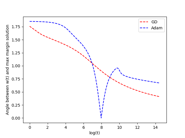
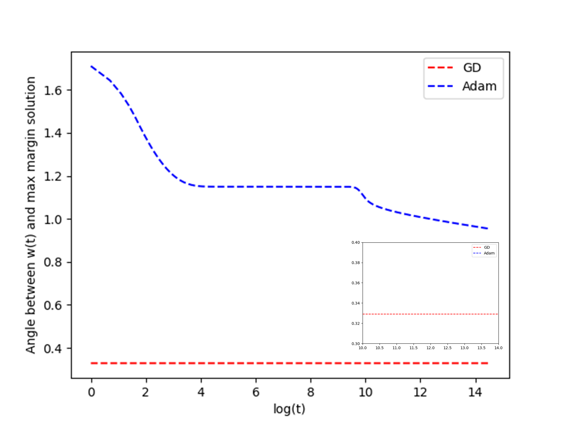
[30] observe that, on a synthetic dataset, the direction of the output parameter by Adam still does not converge to the max-margin direction after iterations (but is getting closer). At the same time, GD seems to converge to the max-margin direction. This seems to contradict with Theorem 4. We reconduct the experiments (please refer to Appendix F.1.2 for details) and found (1). such a phenomenon occurs because a large learning rate is selected, using which GD will also stick in a direction close to the max-margin direction (but not equal); (2). the constructed synthetic dataset is ill-posed, as the non-support data is larger than the support data by order of magnitude (which is also rare in practice). On a well-posed dataset, we observe that both Adam and GD will converge to the max-margin solution rapidly (Figure 1).
We simply introduce the proof idea here and put the full proof in Appendix C. The proof of deterministic Adam is very similar to that of GDM with minor changes in potential functions. Specifically, in Lemma 1 is changed to
and in Lemma 2 is changed to
The rest of the proof then flows similarly to the GDM case.
6.2 What if random sampling is added?
We have obtained the implicit regularization for GDM, SGDM, and deterministic Adam. One may wonder whether the implicit regularization of stochastic Adam can be obtained. Unfortunately, the gap can not be closed yet. This is because an implicit regularization analysis requires the knowledge of the loss dynamics, little of which, however, has been ever known even for stochastic RMSProp (i.e., Adam with in Eq. (3)) with constant learning rates. Specifically, the main difficulty lies in bounding the change of conditioner across iterations, which is required to make the drift term (derived by Taylor’s expansion of the epoch start from ) negative to ensure a non-increasing loss.
On the other hand, if we adopt decaying learning rates , [29] shows close enough to , the following equation holds for stochastic RMSProp (w/o. r) (recall that is the epoch size)
| (8) |
Based on this result, we have the following theorem for stochastic RMSProp (w/o. r):
Theorem 5.
Remark 8 (On the decaying learning rate).
The decaying learning rate is a "stronger" setting compared to the constant learning rate, both in the sense that GDM, SGDM, and deterministic Adam can be shown to converge to the max-margin solution following the same routine as Theorems 2, 3, and 4, and in the sense that we usually adopt constant learning rate in practice.
The proof is on the grounds of a novel characterization of the loss convergence rate derived from Eq. (8), and readers can find the details in Appendix D. Furthermore, the proof can be easily extended to the Stochastic Adaptive Heavy Ball (SAHB) algorithm (proposed by [35]), which can be viewed as a momentum version of RMSProp (but different from Adam) with the following update rule
The proof of Theorem 5 can be easily extended to SAHB, based on the fact that has a simple update, i.e.,
and can be used as a potential function just as the SGDM case.
7 Discussions
Consistency with the Experimental Results. We conduct experiments to verify our theoretical findings. Specifically, we (1). run GD, GDM, SGD, SGDM, and Adam on a synthetic dataset to observe their implicit regularization; (2). run GD and Adam on ill-posed dataset proposed in [30] to verify Theorem 4; (3). run SGD and SGDM on neural networks to classify the MNIST dataset and compare their implicit regularization. The experimental observations stand with our theoretical results. Furthermore, it is worth mentioning that experimental phenomenons that adding momentum will not change the implicit regularization have also been observed by existing literature [30, 20, 38].
Influence of hyperparameters on convergence rates. Our results can be further extended to provide a precise characterization of the influence of the hyperparameters and on the convergence rate of (S)GDM. Specifically, in Appendix E.4, we show that the asymptotic convergence rate of (S)GDM is , where is some constant independent of and . Therefore, increase can lead to a faster convergence rate (with learning rate requirements in Theorems 2 and 3 satisfied). However, changing does not affect the convergence rate, which is also observed in our experiments (e.g., Figure 1). While this seems weird, as replacing gradient with momentum in deep learning often accelerates the training, we hypothesize that such an acceleration appears as the landscape of neural networks is highly non-convex and thus can not be observed in the case considered by this paper.
Gap Between The Linear Model and Deep Neural Networks. While our results only hold for the linear classification problem, extending the results to the deep neural networks is possible. Specifically, existing literature [18, 38] provide a framework for deriving implicit regularization for deep homogeneous neural networks. However, the approach in [18, 38] can not be trivially applied to the momentum-based optimizers, as their proofs require the specific gradient-based updates to lower bound a smoothed margin (c.f., Theorem 4.1, [18]). It remains an exciting work to see how our results can be expanded to GDM and Adam for deep neural networks.
8 Conclusion
This paper studies the implicit regularization of momentum-based optimizers in linear classification with exponential-tailed loss. Our results indicate that for SGD and the deterministic version of Adam, adding momentum will not influence the implicit regularization, and the direction of the parameter converges to the max-margin solution. Our theoretical results stand with existing experimental observations, and developed techniques such as the potential functions may inspire the analyses on other momentum-based optimizers. Motivated by the results and techniques for linear cases in this paper, it has the potential to extend them to the homogeneous neural network in the future. Another topic left for future work is to derive the implicit regularization of constant learning rate stochastic Adam. As discussed in Section 6.2, this topic is non-trivial, and it requires new techniques and assumptions to be developed.
References
- [1] A. Ali, E. Dobriban, and R. Tibshirani. The implicit regularization of stochastic gradient flow for least squares. In International Conference on Machine Learning, pages 233–244. PMLR, 2020.
- [2] X. Chen, S. Liu, R. Sun, and M. Hong. On the convergence of a class of adam-type algorithms for non-convex optimization. In International Conference on Learning Representations, 2018.
- [3] S. De, A. Mukherjee, and E. Ullah. Convergence guarantees for rmsprop and adam in non-convex optimization and an empirical comparison to nesterov acceleration. arXiv preprint arXiv:1807.06766, 2018.
- [4] A. Défossez, L. Bottou, F. Bach, and N. Usunier. A simple convergence proof of adam and adagrad. arXiv preprint arXiv:2003.02395, 2020.
- [5] E. Ghadimi, H. R. Feyzmahdavian, and M. Johansson. Global convergence of the heavy-ball method for convex optimization. In 2015 European control conference (ECC), pages 310–315. IEEE, 2015.
- [6] S. Gunasekar, J. Lee, D. Soudry, and N. Srebro. Characterizing implicit bias in terms of optimization geometry. In International Conference on Machine Learning, pages 1832–1841. PMLR, 2018.
- [7] S. Gunasekar, J. D. Lee, D. Soudry, and N. Srebro. Implicit bias of gradient descent on linear convolutional networks. In Advances in Neural Information Processing Systems, pages 9461–9471, 2018.
- [8] Z. Guo, Y. Xu, W. Yin, R. Jin, and T. Yang. A novel convergence analysis for algorithms of the adam family. arXiv preprint arXiv:2112.03459, 2021.
- [9] Z. Ji, N. Srebro, and M. Telgarsky. Fast margin maximization via dual acceleration. In International Conference on Machine Learning, pages 4860–4869. PMLR, 2021.
- [10] Z. Ji and M. Telgarsky. Gradient descent aligns the layers of deep linear networks. arXiv preprint arXiv:1810.02032, 2018.
- [11] Z. Ji and M. Telgarsky. Directional convergence and alignment in deep learning. arXiv preprint arXiv:2006.06657, 2020.
- [12] Z. Ji and M. Telgarsky. Characterizing the implicit bias via a primal-dual analysis. In Algorithmic Learning Theory, pages 772–804. PMLR, 2021.
- [13] Y. Jiang, B. Neyshabur, H. Mobahi, D. Krishnan, and S. Bengio. Fantastic generalization measures and where to find them. arXiv preprint arXiv:1912.02178, 2019.
- [14] N. S. Keskar, D. Mudigere, J. Nocedal, M. Smelyanskiy, and P. T. P. Tang. On large-batch training for deep learning: Generalization gap and sharp minima. In International Conference on Learning Representations, 2017.
- [15] D. P. Kingma and J. Ba. Adam: A method for stochastic optimization. arXiv preprint arXiv:1412.6980, 2014.
- [16] J. Lin and L. Rosasco. Optimal rates for multi-pass stochastic gradient methods. The Journal of Machine Learning Research, 18(1):3375–3421, 2017.
- [17] Y. Liu, Y. Gao, and W. Yin. An improved analysis of stochastic gradient descent with momentum. Advances in Neural Information Processing Systems, 33, 2020.
- [18] K. Lyu and J. Li. Gradient descent maximizes the margin of homogeneous neural networks. arXiv preprint arXiv:1906.05890, 2019.
- [19] A. Madry, A. Makelov, L. Schmidt, D. Tsipras, and A. Vladu. Towards deep learning models resistant to adversarial attacks. In International Conference on Learning Representations, 2018.
- [20] M. S. Nacson, J. Lee, S. Gunasekar, P. H. P. Savarese, N. Srebro, and D. Soudry. Convergence of gradient descent on separable data. In The 22nd International Conference on Artificial Intelligence and Statistics, pages 3420–3428. PMLR, 2019.
- [21] M. S. Nacson, N. Srebro, and D. Soudry. Stochastic gradient descent on separable data: Exact convergence with a fixed learning rate. In The 22nd International Conference on Artificial Intelligence and Statistics, pages 3051–3059. PMLR, 2019.
- [22] Y. Nesterov. A method for solving a convex programming problem with convergence rate o (1/k2). In Soviet Mathematics. Doklady, volume 27, pages 367–372, 1983.
- [23] B. Neyshabur, R. Tomioka, and N. Srebro. In search of the real inductive bias: On the role of implicit regularization in deep learning. In ICLR, 2015.
- [24] A. Paszke, S. Gross, F. Massa, A. Lerer, J. Bradbury, G. Chanan, T. Killeen, Z. Lin, N. Gimelshein, L. Antiga, et al. Pytorch: An imperative style, high-performance deep learning library. Advances in neural information processing systems, 32:8026–8037, 2019.
- [25] B. T. Polyak. Some methods of speeding up the convergence of iteration methods. Ussr computational mathematics and mathematical physics, 4(5):1–17, 1964.
- [26] Q. Qian and X. Qian. The implicit bias of adagrad on separable data. In Advances in Neural Information Processing Systems, pages 7761–7769, 2019.
- [27] L. Rosasco and S. Villa. Learning with incremental iterative regularization. In Proceedings of the 28th International Conference on Neural Information Processing Systems-Volume 1, pages 1630–1638, 2015.
- [28] R. E. Schapire and Y. Freund. Boosting: Foundations and algorithms. Kybernetes, 2013.
- [29] N. Shi, D. Li, M. Hong, and R. Sun. Rmsprop converges with proper hyper-parameter. In International Conference on Learning Representations, 2021.
- [30] D. Soudry, E. Hoffer, M. S. Nacson, S. Gunasekar, and N. Srebro. The implicit bias of gradient descent on separable data. The Journal of Machine Learning Research, 19(1):2822–2878, 2018.
- [31] W. Su, S. Boyd, and E. Candes. A differential equation for modeling nesterov’s accelerated gradient method: theory and insights. Advances in neural information processing systems, 27, 2014.
- [32] T. Sun, P. Yin, D. Li, C. Huang, L. Guan, and H. Jiang. Non-ergodic convergence analysis of heavy-ball algorithms. In Proceedings of the AAAI Conference on Artificial Intelligence, volume 33, pages 5033–5040, 2019.
- [33] I. Sutskever, J. Martens, G. Dahl, and G. Hinton. On the importance of initialization and momentum in deep learning. In International conference on machine learning, pages 1139–1147. PMLR, 2013.
- [34] M. Tan and Q. Le. Efficientnet: Rethinking model scaling for convolutional neural networks. In International Conference on Machine Learning, pages 6105–6114. PMLR, 2019.
- [35] W. Tao, S. Long, G. Wu, and Q. Tao. The role of momentum parameters in the optimal convergence of adaptive polyak’s heavy-ball methods. arXiv preprint arXiv:2102.07314, 2021.
- [36] M. Telgarsky. Margins, shrinkage, and boosting. In International Conference on Machine Learning, pages 307–315. PMLR, 2013.
- [37] A. Vaswani, N. Shazeer, N. Parmar, J. Uszkoreit, L. Jones, A. N. Gomez, Ł. Kaiser, and I. Polosukhin. Attention is all you need. In Advances in neural information processing systems, pages 5998–6008, 2017.
- [38] B. Wang, Q. Meng, W. Chen, and T.-Y. Liu. The implicit bias for adaptive optimization algorithms on homogeneous neural networks. In International Conference on Machine Learning, pages 10849–10858. PMLR, 2021.
- [39] A. C. Wilson, B. Recht, and M. I. Jordan. A lyapunov analysis of accelerated methods in optimization. Journal of Machine Learning Research, 22(113):1–34, 2021.
- [40] A. C. Wilson, R. Roelofs, M. Stern, N. Srebro, and B. Recht. The marginal value of adaptive gradient methods in machine learning. In Advances in neural information processing systems, pages 4148–4158, 2017.
- [41] S. Xie, R. Girshick, P. Dollár, Z. Tu, and K. He. Aggregated residual transformations for deep neural networks. In Proceedings of the IEEE conference on computer vision and pattern recognition, pages 1492–1500, 2017.
- [42] Y. Yan, T. Yang, Z. Li, Q. Lin, and Y. Yang. A unified analysis of stochastic momentum methods for deep learning. In IJCAI International Joint Conference on Artificial Intelligence, 2018.
- [43] H. Yu, R. Jin, and S. Yang. On the linear speedup analysis of communication efficient momentum sgd for distributed non-convex optimization. In International Conference on Machine Learning, pages 7184–7193. PMLR, 2019.
Supplementary Materials for
“ Does Momentum Change the Implicit Regularization on Separable Data?”
Appendix A Preparations
This section collect definitions and lemmas which will be used throughout the proofs.
A.1 Characterization of the max-margin solution
This section collects several commonly-used characterization of the max-margin solution from [21] and [30].
To start with, we define support vectors and support set, which are two common terms in margin analysis. Recall that in the main text, we assume that without the loss of generality, , .
Definition 2 (Support vectors and support set).
For any , is called a support vector of the dataset , if
Correspondingly, is called a non-support vector if . The support set of is then defined as
The following lemma delivers as an linear combination of support vectors.
Lemma 4 (Lemma 12, [30]).
For almost every datasets , there exists a unique vector , such that can be represented as
| (9) |
where satisfies if , and if . Furthermore, the size of is at most .
By Lemma 4, we further have the following corollary:
Corollary 1.
For almost every datasets , the unique given by Lemma 4 further satisfies that for any positive constant , there exists a non-zero vector , such that, , we have
| (10) |
Proof.
For the stochastic case, we will also need the following lemma when we calculate the form of parameter at time .
Lemma 5 (Lemma 5, [21]).
Let be the random subset used in SGDM (w/. r). Almost surely, there exists a vector
where satisfies for any , and . As for SGDM (w/o. r), the a.s. condition can be removed.
A.2 Preparations of the optimization analysis
This section collects technical lemmas which will be used in latter proofs. We begin with a lemma bounding the smooth constants if the loss is bounded.
Lemma 6.
If loss satisfies (D) in Assumption 3, then for any , if , then we have is smooth at point , where . Furthermore, is globally smooth over the set .
Proof.
Since is positive, we have ,
which leads to , and is smooth at .
Furthermore, since , for any two parameters and close enough to ,
Now if and both belong to , we have for any , , and . Following the same routine as the locally smooth proof, we complete the second argument.
The proof is completed. ∎
Based on Assumption 2, we also have the following lemma characterizing the relationship between loss and its derivative when is large enough.
Lemma 7.
Let loss satisfy Assumption 2. Then, there exists an large enough and a positive real , such that, , we have
Proof.
By Assumption 2, there exists a large enough , such that , we have
| (11) |
The proof is completed. ∎
By Lemma 7, we immediately get the following corollary:
Corollary 2.
Let loss satisfy Assumption 2. Then, there exist positive reals and , such that, for any satisfying either or , we have
Proof.
We start with the case . By simple calculation, we have
| (12) |
and
| (13) |
By Assumption 2, we have there exists a constant , s.t., any with satisfies . Let . We then have if , then (), and thus . Combing Eqs. (12) and (13), we then have
Similarly, as for the case , we have there exists a constant , s.t., any with satisfies . Let and the rest of the proof follows the same routine as the first case.
The proof is completed. ∎
The following lemma bridges the second moment of with its squared first moment.
Lemma 8.
Let the dataset satisfies the separable assumption 1. Let be a random subset of with size sampled independently and uniformly without replacement. Then, at any point , we have
Proof.
To start with, notice that
Therefore, the first inequality can be directly obtained by Cauchy-Schwartz’s inequality. To prove the second inequality, we first calculate the explicit form of .
Therefore,
| (14) |
On the other hand,
where Eq. () is due to , and .
Therefore,
| (15) |
In the following lemma, we show the updates of GDM, Adam, and SGDM are all non-zero.
Lemma 9.
Regardless of GDM, Adam, or SGDM, the updates of all steps are non-zero, i.e.,
Proof.
We start with the alternative forms of the update rule of GDM, Adam, and SGDM using the gradients along the trajectory respectively. For GDM, by Eq. (1), the update rule can be written as
| (16) |
Similarly, the update rule of SGDM can be written as
| (17) |
while the update rule of Adam can be given as
| (18) |
On the other hand, by the definition of empirical risk , the gradient of at point can be given as
| (19) |
By Eq. (19) and Eq. (16), we further have for GDM,
| (20) |
By Assumption 1, there exists a non-zero parameter , such that, , . Therefore, by executing inner product between Eq. (20) and , we have
where Eq. is due to . This complete the proof for GDM.
Similarly, for SGDM, we have
which completes the proof of SGDM.
For Adam, we have
which completes the proof of Adam.
The proof is completed. ∎
Appendix B Implicit regularization of GD/SGD with momentum
This section collects the proof of the implicit regularization of gradient descent with momentum and stochastic gradient descent with momentum. The analyses of this section hold for almost every dataset, and the "almost every" constraint is further moved in Section E.1.
B.1 Implicit regularization of GD with Momentum
This section collects the proof of Theorem 2.
B.1.1 Proof of the sum of squared gradients converges
To begin with, we will prove the sum of squared norm of gradients along the trajectory is finite for gradient descent with momentum. To see this, we first define the continuous-time update rule as
We then prove a generalized case of Lemma 1 for any .
Lemma 10 (Lemma 1, extended).
Proof of Lemma 10.
We prove this lemma by reduction to absurdity.
Concretely, let be the smallest positive integer time such that there exists an , such that Eq. (21) doesn’t hold. Let . By continuity, Eq. (21) holds for .
We further divide the proof into two cases depending on the value of .
Case 1: : For any , we have Eq. (21) holds for . Specifically, we have
which further leads to
Since is non-negative, we have
By Lemma 6, we have is smooth at . Therefore, by Taylor’s expansion for at point , we have for small enough
| (22) |
where Eq. is due to a simple rearrangement of the update rule of gradient descent with momentum (Eq. (1)), i.e.,
| (23) |
Inequality is due to Cauchy Schwarz’s inequality and arithmetic-geometric average inequality, and Inequality is due to
Here the inequality is due to that tend to as tend to zero, which is a negative constant by Lemma 9, and is .
Case 2: : Same as Case 1, we have for any ,
which further leads to
| (24) |
On the other hand, by the definition of , we have for any , we have Eq. (21) holds for , which by continuity further leads to Eq. (21) holds for . Therefore, , otherwise, Eq. (21) holds for , which contradicts the definition of .
Combining Eq. (21) with and Eq. (24), we further have
Consequently, for any
and by Lemma 6, we then have is smooth at , which further by Taylor’s expansion leads to
where Eq. () follows the same routine as Case 1, Eq. () is due to the definition of and , and Eq. () is due to , and (given by Lemma 9).
By the continuity of , for any small enough , Eq. (21) holds for , which contradicts to the definition of .
The proof is completed. ∎
By Lemma 1, one can easily obtain the sum of the squared norms of the updates across the trajectory converges.
Proof.
Taking leads to
By triangle inequality, we further have
where Eq. () is due to Cauchy-Schwartz’s inequality.
The proof is completed. ∎
By the negative derivative of the loss and the separable data, we can finally prove the sum of squared gradient converges.
Corollary 4.
Let all conditions in Theorem 2 hold. We have, .
Proof.
By the exponential-tailed assumption of the loss (Assumption 2), we further have the following corollary.
Corollary 5.
Let all conditions in Theorem 2 hold. Then, , and
Consequently, there exists an large enough time , such that, , , we have , and
B.1.2 Parameter dynamics
To prove Theorem 2, we only need to show has bounded norm for any iteration . Letting in Corollary 1, we obtain an constant vector satisfying Eq. (10). Define
| (27) |
As is a constant vector, that has bounded norm is equivalent to has bounded norm. As discussed in the main body of the paper, we then propose an equivalent proposition of is bounded, and further prove this proposition is fulfilled. Specifically, we have
Lemma 11.
Let all conditions in Theorem 2 hold. Then, is bounded if and only if the function is upper bounded, where is defined as
| (28) |
Furthermore, for almost every dataset, we have is upper bounded.
As the proof is rather complex, we separate it into two sub-lemmas. We first prove is bounded if and only if function is upper bounded.
Lemma 12 (First argument in Lemma 11).
Let all conditions in Theorem 2 hold. Then, is bounded if and only if function is upper bounded.
Proof.
We start the proof by showing that has bounded absolute value.
By the definition of , we have
which further indicates
Therefore, the absolute value of can be bounded as
where Inequality is due to the Inequality of arithmetic and geometric means, and Inequality is due to Corollary 3 and .
Therefore, is upper bounded is then equivalent to is upper bounded. Now if is upper bounded, we will prove is bounded by reduction to absurdity.
Suppose that has unbounded norm. By Corollary 3, we have , and there exists a large enough time , such that for any . On the other hand, since is unbounded from above, there exists an increasing time sequence , , such that
Therefore, we have
which leads to contradictory, and completes the proof of necessity.
On the other hand, if is upper bounded, since is also upper bounded, we have is upper bounded, which completes the proof of sufficiency.
The proof is completed. ∎
Therefore, the last piece of this puzzle is to prove is upper bounded .
Lemma 13 (Second argument in Lemma 11).
Let all conditions in Theorem 2 hold. Then, for almost every dataset, we have that is upper bounded.
Proof.
We start the proof by calculating . For any , we have
On the other hand, by simply rearranging the update rule Eq. (1), we have
| (29) |
which further indicates
Denote , and . We then prove respectively and are upper bounded.
Then we only need to prove .
To begin with, by adding one additional term into , we have
On the other hand, by direct calculation of the gradient, we have
where Eq. () is due to the definition of (Eq. (10) with ).
Denote
and
We then analysis these two terms respectively. As for , due to , we have
By Corollary 5, we further have
which further indicates
where in Eq. is defined as
| (32) |
As , we have
| (33) |
For each term () in , we divide the analysis into two parts depending on the sign of .
Since , we further have
where Eq. () is due to , .
Specifically,
Therefore,
Case 2: . Similar to Case 1., in this case we have
Specifically, if ,
where Eq. () is due to if ,
If , we have
Therefore, when is large enough, , which by leads to
If ,
For large enough , , and
Therefore, in Case 2., for large enough , we have
Combining Case 1. and Case 2., we conclude that
which further yields
| (34) |
We are now ready to prove Theorem 2.
B.2 Implicit regularization of SGDM
This section collects the proof of Theorem 3. Following the same framework as Appendix B.1, we will first prove that the sum of the squared gradient norms along the trajectory is finite. One may expect is a Lyapunov function of SGDM. However, due to the randomness of the update rule of SGDM, may no longer decrease (we will show this in the end of Appendix B.2, please see Appendix B.2.3 for explanation).
B.2.1 Loss dynamics
Recall that in the main text, we define as
| (35) |
where the update of is given by . We then prove Lemma 3, which indicates is a proper choice of Lyapunov function.
Proof of Lemma 3.
We start the proof by applying the Taylor’s expansion of at the point to the point . Concretely, by Assumption 3. (S), we have
which by Eq. (35) leads to
| (36) |
Taking the expectation of Eq. (36) with respect to conditioning on (recall that is the sub-sigma algebra over the mini-batch sampling, such that , is adapted with respect to the sigma algebra flow ), we have
| (37) |
where Eq. is due to that is uniquely determined by given , Eq. is due to is uniquely determined by , and Inequality. is due to Lemma 8.
Therefore, we have
where is a positive constant that will be specified latter.
By Assumption 3. (S), is -smooth, which further leads to
| (38) |
where Inequality is due to by Eq. (35), Inequality is due to triangular inequality, and Inequality () is due to Cauchy-Schwartz Inequality.
Combining Eqs. (37) and (38), we have
which by taking expectation with respect to leads to
where the last inequality is due to Lemma 8. Lettting then leads to
By the learning rate upper bound , summing the above inequality over then leads to
where .
The proof is completed. ∎
As is upper bounded, we have the following corollary given by Lemma 3.
Corollary 6.
B.2.2 Parameter dynamics
Similar to the case of GDM, we define as the solution of Eq. (10) with . We also let be given by Lemma 5, and define in this case as
| (40) |
As is a constant vector, and as , we have has bounded norm if and only if is upper bounded. Similar to the GDM case, we have the following equivalent condition of that is bounded.
Lemma 14.
Let all conditions in Theorem 3 hold. Then, is bounded almost surely if and only if function is upper bounded almost surely, where is defined as
| (41) |
Proof.
To begin with, we prove that almost surely is upper bounded for any . By Corollary 6, we have almost surly
On the other hand, for any , we have
Therefore, we have almost surely,
which further leads to almost surely
Therefore, is upper bounded almost surely is equivalent to is upper bounded, which can be shown to be equivalent with is bounded following the same routine as Lemma 11.
The proof is completed. ∎
As the case of GDM, we only need to prove is upper bounded to complete the proof of Theorem 3.
Lemma 15.
Let all conditions in Theorem 3 hold. Then, for almost every dataset, we have is upper bounded.
Proof.
Combining the above two equations, we further have
which further indicates
Therefore, we only need to prove . By directly applying the form of , we have
Let , and . We will investigate these two terms respectively.
As , , a.s., we have a.s., there exists a large enough time , s.t., , ,
Therefore,
where Inequality. is due the definition of (Eq. (32)), Inequality. () is due to , and Eq. is due to . Thus,
On the other hand, can be rewritten as
If , we have for ,
where Eq. is due to , and Eq. () is due to .
On the other hand, if , we have
Specifically, if ,
where Eq. () is due to that as and as , there exists a large enough time , s.t., , under the circumstance , and .
If , then, for large enough , , , and
If , then for large enough time , , , and
Conclusively, if , for large enough , we have
which further indicates, for large enough , we have
which indicates
Therefore,
The proof is completed. ∎
B.2.3 Explanation for proper lyapunov function
Based on the success of applying Lyapunov function to analyze gradient descent with momentum, it is natural to try to extend this routine to analyze stochastic gradient descent with momentum. However, in this section, we will show such Lyapunov function is not proper to analyze SGDM as this will put constraints on the range of the momentum rate . Specifically, at any step , since the loss is smooth at , we can expand the loss in the same way as the GDM case:
By taking expectation with respect to conditioning on for both sides, we further obtain
where Eq. is becasue due to the definition of SGDM (Eq. (2)). Rearranging the above inequality and taking expectations of both sides with respect to leads to
| (42) |
On the other hand, we wish to obtain some positive constant from Eq. (42), such that (at least),
| (43) |
which requires to lower bound by . However, in general cases, is only upper bounded by (Holder’s Inequality), although in our case, can be bounded as
while by the separability of the dataset and that the loss is non-increasing, can be bounded as
| (44) |
By Eqs. (42) and (44), we have that to ensure Eq. (43), it is required that
which puts additional constraint on as
Specifically, the upper bound becomes close to when becomes large, and constrains in a small range.
Appendix C Implicit regularization of deterministic Adam
This section collects the proof of the convergent direction of Adam, i.e., Theorem 4. The methodology of this section bears great similarity with GDM, although the preconditioner of Adam requires specific treatment for analysis. The proof is still divided into two stages: (1). we first prove the sum of squared gradients along the trajectory is finite. Additionally, we prove the convergent rate of loss is ; (2). we prove has bounded norm. Before we present these two stages of proof, we will first give the required range of for which Theorem 3 holds. The analyses of this section hold for almost every dataset, and the "almost every" constraint is further moved in Section E.1.
C.1 Choice of learning rate
Let be the smooth parameter over given by Assumption 3. (D). Let (). The "sufficiently small learning rate" in Theorem 3 means
To ensure is well-defined, we need to prove
and we introduce the following technical lemma:
Lemma 16.
Define , . We have is decreasing with respect to . Furthermore, for any , we have
| (45) |
Proof.
The left side of the above inequality is no smaller than 1, while the right side is no larger than 1, which completes the proof. ∎
We are now ready to prove is well-defined. First of all, for every , we have
| (46) |
where Eq. () is by Lemma 16 and .
On the other hand, we have
| (47) |
C.2 Sum of gradients along the trajectory is bounded
We start with the following lemma, which indicates is a proper Lyapunov function for Adam.
Lemma 17.
Let all conditions in Theorem 4 hold. Then, for any ,
| (48) |
Proof.
We start with the case . To begin with, we have is smooth around . By definition is non-increasing with respect to , and since is also non-increasing, we have
which further indicates when is small enough,
where in Eq. () we denote , and the last inequality is due to , and is positive.
Now if there exists an , such that Eq. (48) fails, we denote . We have , and the equality in Eq. (48) holds for . Therefore, we have for any ,
which by Lemma 6 leads to is smooth (thus smooth) over the set , and
| (49) |
where the second-to-last inequality is due to (by Lemma 9) and , while the last inequality is due to
Eq. (49) contradicts the fact that the equality in Eq. (48) holds for , which completes the proof of .
If , following the similar routine as , we also prove Eq. (48) by reduction to absurdity. If there exist and such that Eq. (48) fails. Denote as the smallest time such that there exists an such that Eq. (48) fails for and . By Lemma 9, is positive, and strict inequality in Eq. (48) holds for and , which by continuity leads to
Then, for any , we have
On the other hand, for any time , we have
| (50) |
On the other hand, for , we have
| (52) |
Therefore, by Lemma 6, is smooth (thus smooth) over the set , which further leads to
where Eq. is due to an alternative form of the Adam’s update rule:
| (53) |
Inequality is due to
and , and Inequality is due to
, and .
This contradicts to that the equality in Eq. (48) holds for .
The proof is completed. ∎
As and , we have the following corollary based on Lemma 1.
Corollary 7.
Let all assumptions in Theorem 4 hold. Then, for large enough , we have
| (54) |
Consequently, we have
| (55) |
The proof of Corollary 7 relies on the following classical lemma on the equivalence between the convergence of two non-negative sequence. The proof is omitted here and can be found in [38].
Lemma 18 (c.f. Lemma 27, [38]).
Let be a series of non-negative reals, and be a positive real. Then, is equivalent to .
Proof of Corollary 7.
Based on Corollary 7, we can further prove Lemma 19, characterizing the convergent rate of loss directly.
Lemma 19.
Let all conditions in Theorem 4 hold. Then, , and .
Proof of Lemma 19.
To begin with, Eq. (53) indicates
| (57) |
On the other hand, by Corollary 7,
which following the same routine as Corollary 6 leads to
Therefore, by Lemma 7, there exists a large enough time , such that ,
which by the separable assumption further leads to
| (58) |
Combining Eq. (26) and the above inequality, we have
| (59) |
On the other hand, by Eq. (56), we have
Therefore, there exists large enough time , such that ,
and thus,
| (60) |
Rearranging Eq. (54) leads to
which further indicates
Denote as
We then have
which leads to
Due to Eq. (58), we further have , which indicates
Therefore, for any , we have , which by is exponential-tailed leads to , and thus . Also, since , we have , which further leads to , and thus .
Finally, we have
which leads to . Similarly, we have , component-wisely. As and , we have
The proof is completed. ∎
C.3 Parameter dynamics
By Lemma 4, there exists a solution as the solution of Eq. (10) with . Define as
| (61) |
and we only need to prove is bounded over time. We then prove has bounded norm. Specifically, we will prove the following lemma:
Lemma 20.
Let all conditions in Theorem 4 hold. Then, is bounded if and only if is upper bounded, where is defined as follows.
Furthermore, we have is upper bounded.
Similar to GDM, the proof of Lemma 20 is divided into two parts, each focus on one claim of it. We start with the first claim.
Lemma 21.
Let all conditions in Theorem 4 hold. Then, is bounded if and only if is upper bounded.
Proof.
The proof is completed. ∎
We conclude the proof of Theorem 4 by showing is upper bounded.
Lemma 22.
Let all conditions in Theorem 4 hold. Then, is upper bounded.
Proof.
is upper bounded is equivalent to . We then prove this lemma by calculating directly.
where Eq. is due to a simple rearranging of the update rule of Adam, i.e.,
On the one hand, as ,
On the other hand,
where Eq. () is due to .
Furthermore, following exactly the same routine as Lemma 13, we have
The proof is completed. ∎
Appendix D Implicit regularization of RMSProp (w/o. r) with decaying learning rate
This section collects the proof of Theorem 5. To begin with, we formally define RMSProp (w/o. r) as follows to facilitate latter analysis: for each , divide the sample set into subsets uniformly and i.i.d., and let
| (64) |
Here the is the individual loss average over , i.e., , where is the batch size. With Eq. (64), we restate the loss convergence result in [29] as the following proposition.
Proposition 1 (Corollary 4.1 in [29], restated).
Suppose is non-negative and -smooth. Furthermore, assume that there exists a constant , s.t., ,
| (65) |
and
Then, RMSProp (w/o. r) with decaying learning rate satisfies
Corollary 8.
Applying relationship between and of the exponentially-tailed loss, we can further obtain the loss convergent rate.
Lemma 23.
Let all the conditions in Theorem 5 hold. Then, we have
Proof.
To begin with, we show that there exists an increasing positive integer sequence , and by reduction to absurdity. Otherwise, suppose there exists a positive integer , such that , . Therefore, for , we have
Let be large enough, we have , which contradicts Corollary 8.
Denote . By the above discussion, contains an increasing positive integer sequence. We then prove that if and , where is defined as
( and is defined in Corollary 2), there exists , and . We slightly abuse the notation and let . If , this claim trivially holds. Otherwise, as , we have
which by Corollary 2 further leads to
Therefore, by Corollary 8, we have
which by further leads to
and thus . As , we have
which leads to
and thus . By the inductive method, we have for any ,
If , applying into the above equation leads to
and
which leads to , and contradicts the definition of . Therefore, we have .
As contains an increasing integer sequence, there exists an , s.t., and . Let be any positive integer larger than and let be the largest integer smaller than and belongs to . We have , and by the above discussion. Therefore, we have
The proof is completed. ∎
As a corollary, we can obtain an asymptotic estimation of .
Corollary 9.
Let all the conditions in Theorem 5 hold. Then, we have
Proof.
On the other hand, we have
As is smooth, we further have
Combining the above two equations, we have
The proof is completed. ∎
Proof of Theorem 5 (for almost every dataset).
To begin with, define , where is the solution of Eq. (10) with , and is given by Lemma 5. As in the case of GDM, SGDM, and Adam (w/s), has bounded norm if and only if has bounded norm. Also, it is a sufficient condition to ensure is bounded that both and .
As for , we have
where Inequality is due to
, and .
As for , we have
| (66) |
On the other hand, as
we have . Also, we have , and thus . Combining these estimations, we have
and
Therefore,
As for the last term in Eq. (66), we have
Then, following the same routine as Lemma 15, we have
The proof is completed. ∎
Appendix E Applications & Extensions
E.1 Deriving the conclusion for every dataset
In Sections 4, 5, and 6, we only derive the implicit regularization for almost every dataset, but not all the separable datasets. In this section, we show that the "almost every" condition can be removed as the following theorem.
Theorem 6.
We have the following conclusions:
-
•
For GDM, let all the conditions in Theorem 2 hold. Then, GDM converges to the max-margin solution;
-
•
For SGDM sampling with replacement, let all the conditions in Theorem 3 hold. Then, SGDM (w/. r) converges to the max-margin solution (the same for SGDM (w/o. r), except a different learning rate upper bound);
-
•
For deterministic Adam, let all the conditions in Theorem 4 hold. Then, Adam (w/s) converges to the max-margin solution;
-
•
For RMSProp (w/o. r), let all the conditions in Theorem 5 hold. Then, RMSProp (w/o. r) converges to the max-margin solution.
It can be easily observe that to prove Theorem 6, the analysis of Stage I of every optimizer still works. Therefore, we only need to change Stage II. As the analyses of Stage II are highly overlapped for different optimizers, we only provide a proof of GDM.
To begin with, we present some notations and results on the structure of the separable dataset from [30].
Let , and . We then recursively define the index sets , , , and :
where (we also denote ), and is defined as the max-margin solution of dataset (that is, the transferred data with index in projected through matrix ):
| (67) |
The existence of the is guaranteed by the KKT condition of Eq. (67). The above procedure will produce a sequence , , , and will stop at if is empty (if the sequence is infinite, we let ). For every , we have is non-zero, and is non-empty, which leads to , and .
The following lemma characterize the structure of the dataset.
Lemma 24 (Lemma 17, [30]).
, we can find a unique , such that
and .
We then have the following lemma:
Lemma 25 (Lemma 18, [30]).
, the equations
under the constraints and have the unique solution .
We then denote
where
Similar to Eq. 28, we define
We then have the following lemma parallel to Lemma 11:
Lemma 26.
Let all conditions in Theorem 2 hold. We have is finite. Furthermore, is finite if and only if is finite, and consequently is finite.
Proof.
The proof of the second argument follows the same routine as the proof of the first argument in Lemma 11, and we omit it here.
As for the first argument, we have
where the first term can be shown to be finite similar to Lemma 11, while the second term is finite by Lemma 14 in [30].
The proof is completed. ∎
E.2 Implicit regularization of SGDM (w/o. r)
This section provides formal description of the implicit regularization of SGDM (w/o. r) and its corresponding proof. To begin with, we would like to provide a formal definition of SGDM (w/o. r). SGDM (w/o. r) differs from SGDM by applying sampling without replacement to obtain in Eq. (2). Specifically, let . For any , we call time series the -th epoch, and during the -th epoch, the dataset is randomly uniformly divided into parts , with . The implicit regularization of SGDM (w/o. r) is then stated as the following theorem:
Theorem 7.
The without-replacement sampling method leads to the direction of every trajectory of mini-SGDM converge to the max-margin solution, compared to the same conclusion holds for SGDM a.s.. We prove the theorem following the same framework of GDM, by proceeding with two stages.
Stage I. The following lemma proves is an Lyapunov function for SGDM (w/o. r) and without the a.s. condition.
Lemma 27.
Let all conditions in Theorem 7 hold. Then, we have
Proof.
By the Taylor Expansion of at , we have
| (68) |
On the other hand, for any , we have
which by is small enough further indicates
Applying the same analysis to recursively, we finally obtain
| (69) |
Therefore,
| (70) |
Similarly, one can obtain
| (71) |
Summing the above inequality over and setting small enough leads to the conclusion.
The proof is completed. ∎
E.3 Extension to the multi-class classification problem
As mentioned in Section 3, despite all the previous analyses are aimed at the binary classification problem, they can be naturally extended to the analyses multi-class classification problem. Specifically, in the linear multi-class classification problem, for any in the sample set , the (individual) logistic loss with parameter is denoted as
Correspondingly, dataset is separable if there exists a parameter , such that , we have , . The multi-class max-margin problem is then defined as
where denotes the Frobenius norm. Denote as the max-margin solution, we have SGDM and Adam (w/s) still converges to the direction of .
Theorem 8.
For linear multi-class classification problem using logistic loss and almost every separable data, with a small enough learning rate, and (for Adam (w/s)), SGDM and Adam (w/s) converge to the multi-class max-margin solution (a.s. for SGDM SGDM (w/. r)).
Here we use several notations and lemmas from [30]. We define , , () satisfying , and , where is the identity matrix with dimension . We still consider the normalized data, i.e., , . Then, the individual loss of sample can be then represented as
Furthermore, the gradient of training error at has the form
and the Hessian matrix of can be represented as
one can then easily verify all absolute value of the eigenvalues of is no larger than , which indicates is -globally smooth.
On the other hand, the separable assumption leads to , , which further indicates
Let , following the similar routine as the binary case, we have for a random subset of sampled uniformly without replacement with size , we have
| (72) |
Similarly, we have for any positive real series ,
| (73) |
The proofs of Stage I can then be obtained with Lyapunov functions unchanged and by replacing the corresponding lemmas using Eq. (72) and Eq. (73).
As for the proofs of Stage II, the Lyapunov functions are still the same, while we only need to prove the sum of (for GDM, for SGDM, for Adam). For the multi-class case using GDM, We present the following lemma from [30], while the other two cases can be proved similarly:
Lemma 28 (Part of the proof of Lemma 20, [30]).
If as , and , we have the sum of is upper bounded.
The proof of Theorem 8 is then completed.
E.4 Precisely characterize the convergence rate
Theorem 2 and Theorem 3 can be further extended to precisely characterize the asymptotic convergence rate for (S)GDM as the following theorem.
Theorem 9.
The proof follows exactly the same routine as (Corollary 1, [20]) and we omit it here.
Appendix F Experiments
This section collects several experiments supporting our theoretical results.
F.1 Experiments on linear model
F.1.1 Comparing the training behavior of (S)GD, (S)GDM, deterministic Adam and RMSProp
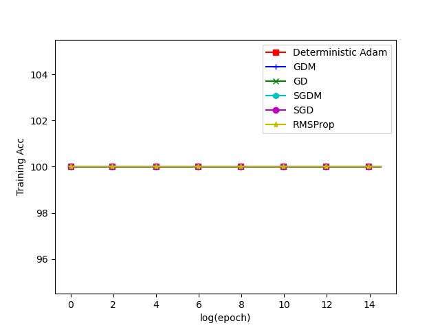
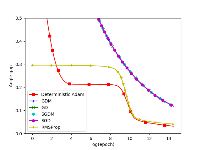
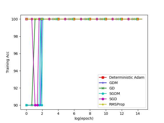
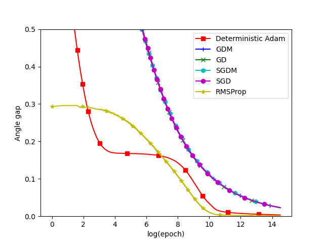
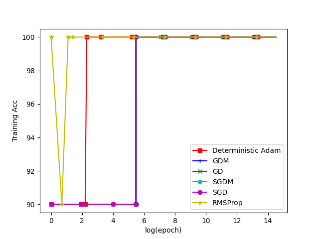
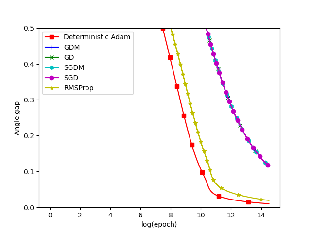
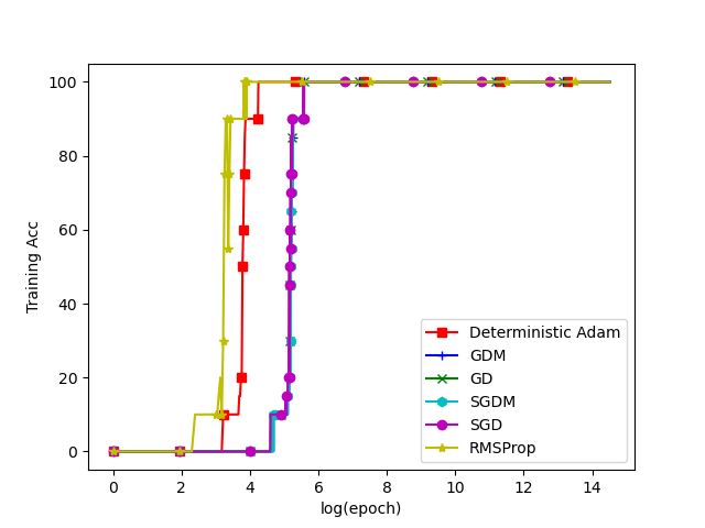
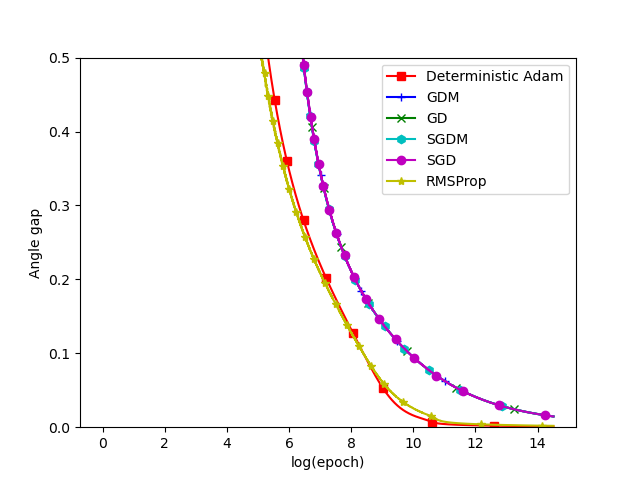
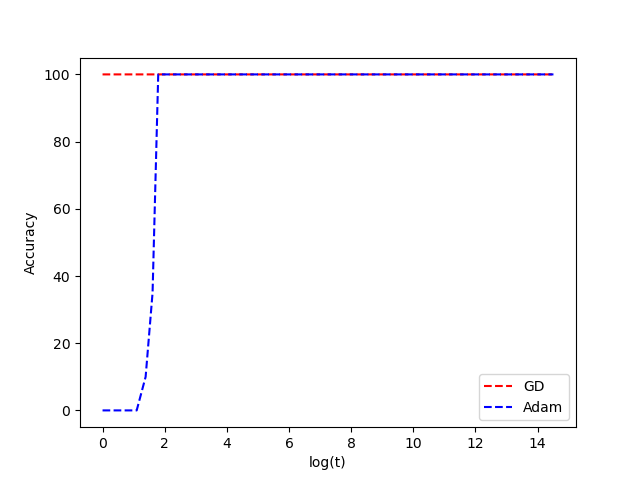
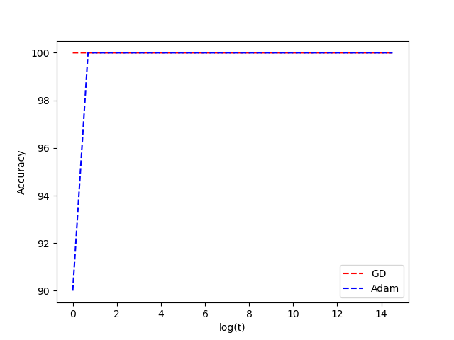
The experiments in this section is designed to verify our theoretical results, i.e., Theorems 2, 3, 4, and 5. We use the synthetic dataset in (Figure 1, [30]) and logistic loss, and run (S)GD, (S)GDM, deterministic Adam and stochastic RMSProp over it with different learning rates and different random seeds (for random initialization, random samples despite the support sets ), and random mini-batches. Both the angle between the output parameter and max-margin solution and the training accuracy are plotted in Figure 2. The observations can be summarized as follows:
-
•
With proper learning rates, all of (S)GD, (S)GDM, deterministic Adam and stochastic RMSProp converge to the max-margin solution, which supports our theoretical results;
-
•
(Similarity between (S)GD and (S)GDM). The asymptotic training behaviors of GD, SGD, GDM and SGDM are highly similar, which supports our Theorem 9.
-
•
(The acceleration effect of Adam). Deterministic Adam and stochastic RMSProp achieve smaller angle with the max-margin solution under the same number of iterations.
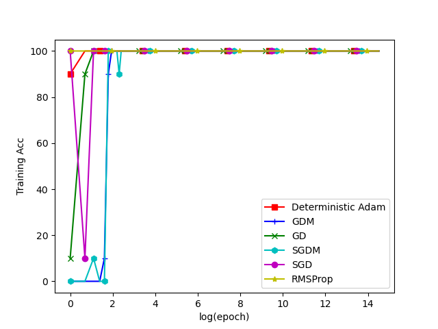
F.1.2 Adam on ill-posed dataset
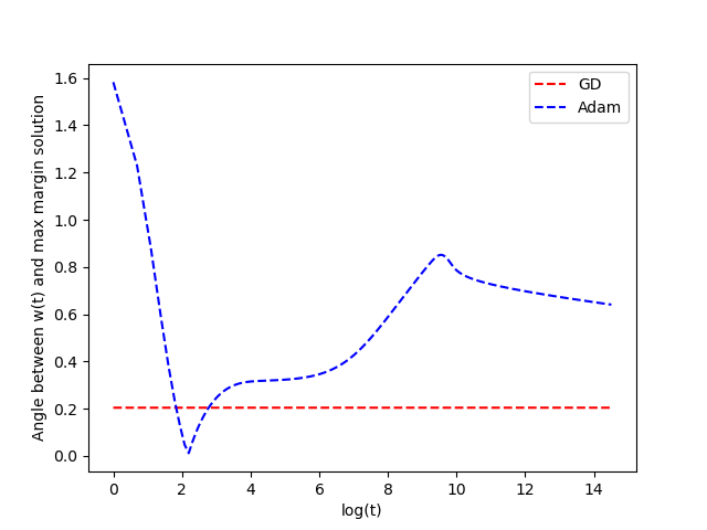
In Figure 3 of [30], an ill-posed synthetic dataset is proposed to support the argument "Adam does not converge to max-margin solution", which contradicts to the theoretical results of this paper. We re-conduct the experiment of Figure 3 in [30] with the same ill-posed synthetic dataset with different learning rates and different random seeds as Figure 3. Figure 3. (f) is similar to Figure 3 in [30], where with learning rate and random seed , the angle of GD to the max-margin solution is smaller than Adam all the time. However, it can be observed from the amplified figure that the angle of GD keeps still and above all the time, meaning that GD doesn’t converge to the max-margin solution under this setting. However, the angle of Adam to the max-margin solution still keeps decreasing and it’s unreasonable to claim "Adam doesn’t converge to the max-margin solution" in this case (the same issue exists in Figure 3 in [30]). Also, as we mentioned at the beginning of this section, this dataset is ill-posed, which is due to the imbalance between the two components of the data (for all data in the dataset, is always smaller than , while is larger than (and even larger than despite two data in the dataset)), which requires smaller learning rate. To tackle this problem, we need to tune down the learning rate. By Figure 3. (b) and (d), after scaling down the learning rate, both GD’s angle and Adam’s angle keep decreasing.
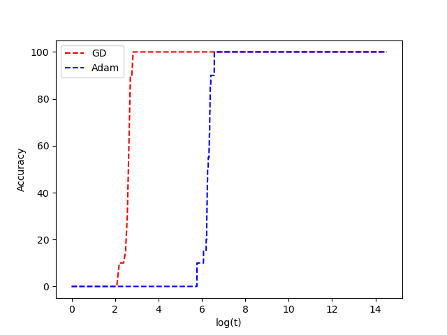

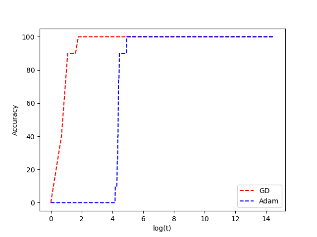
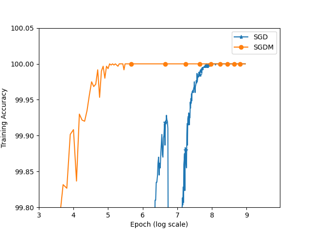
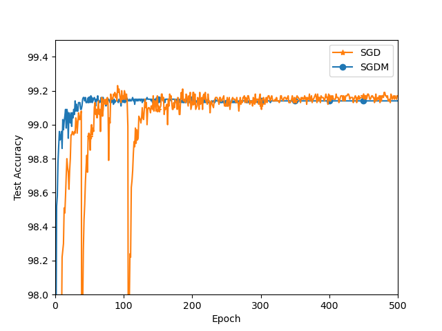
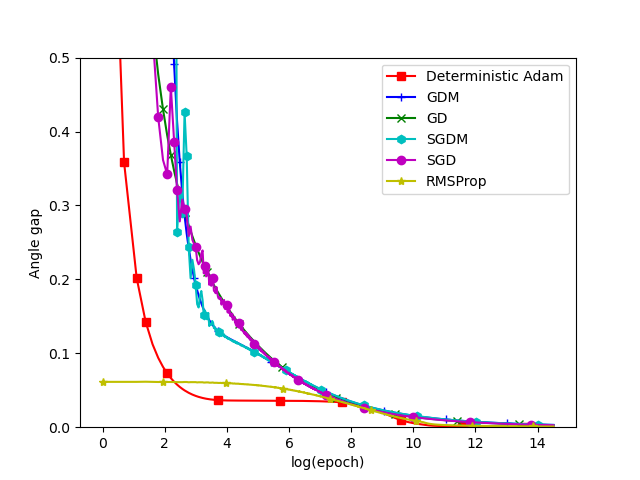
F.2 Evidence from deep neural networks
We conduct an experiment on the MNIST dataset using the four layer convolutional networks used in [18, 38] (first proposed by [19]) to verify whether SGD and SGDM still behave similarly in (homogeneous) deep neural networks. The learning rates of the optimizers are all set to be the default in Pytorch. The results can be seen in Figure 4. It can be observed that (1). SGDM achieves similar test accuracy compared to SGD while (2). SGDM converges faster than SGD.