ModeRNN: Harnessing Spatiotemporal Mode
Collapse in Unsupervised Predictive Learning

Abstract

Learning predictive models for unlabeled spatiotemporal data is challenging in part because visual dynamics can be highly entangled in real scenes, making existing approaches prone to overfit partial modes of physical processes while neglecting to reason about others. We name this phenomenon spatiotemporal mode collapse and explore it for the first time in predictive learning. The key is to provide the model with a strong inductive bias to discover the compositional structures of latent modes. To this end, we propose ModeRNN, which introduces a novel method to learn structured hidden representations between recurrent states. The core idea of this framework is to first extract various components of visual dynamics using a set of spatiotemporal slots with independent parameters. Considering that multiple space-time patterns may co-exist in a sequence, we leverage learnable importance weights to adaptively aggregate slot features into a unified hidden representation, which is then used to update the recurrent states. Across the entire dataset, different modes result in different responses on the mixtures of slots, which enhances the ability of ModeRNN to build structured representations and thus prevents the so-called mode collapse. Unlike existing models, ModeRNN is shown to prevent spatiotemporal mode collapse and further benefit from learning mixed visual dynamics.

1 Introduction

Predictive learning is an unsupervised learning method that has shown the ability to discover latent structures of unlabeled spatiotemporal data. However, in practice, the spatiotemporal data often contains a variety of visual dynamics, which are mainly reflected in the richness of spatial correlations and movement trends, as well as the diversity of interactions between multiple objects (see Figure 1). It remains a challenge for existing predictive models to fully capture these spatiotemporal modes in a completely unsupervised manner using regular forward modeling mechanisms, such as recurrent update (Shi et al., 2015), autoregression (Kalchbrenner et al., 2017), and 3D convolutions (Wang et al., 2019a), while ignoring the inherent differences in dynamics among data samples. For clarity, in the following discussion, spatiotemporal modes are considered to have the following properties:

1. Multiple spatiotemporal modes naturally exist in the dataset and are unknown before model training. They can be viewed as prototypes of space-time representations. For simplicity, each sequence corresponds to a single spatiotemporal mode.

2. Multiple modes share a set of hidden representation subspaces (referred to as “spatiotemporal slots”) and have different compositional structures over the spatiotemporal slots.

We observe that if the predictive model experiences multiple complex modes in spacetime during training, the learning processes of different modes may affect each other, resulting in ambiguous prediction results. Figure 1(a) provides an example that the predictive model responds effectively only to certain visual dynamics, from which it learns biased prior knowledge (e.g., collision-free), and generates future frames arbitrarily based on these priors while neglecting to reason about other possibilities of latent modes. We name this phenomenon spatiotemporal mode collapse.

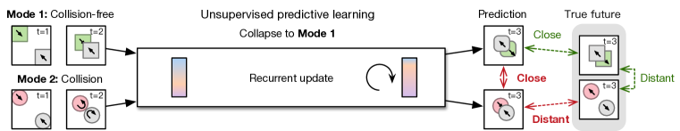
(a) Learning RNNs under highly mixed modes of visual dynamics (e.g., collision-free vs. collision) may lead to spatiotemporal mode collapse, i.e., the predictions of some modes are severely affected by the presence of others.

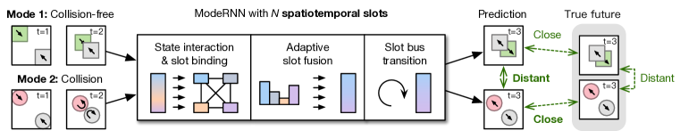
(b) ModeRNN tackles mode collapse by learning the compositional structures of visual dynamics through a set of spatiotemporal slots. The three modules in each recurrent unit of ModeRNN will be discussed later.

Figure 1: Illustration of spatiotemporal mode collapse and our approach.

Unlike the widely concerned mode collapse problem in generative adversarial networks, the above issue is previously considered to be less likely to occur in the generation of future frames conditioned on sequential observations, because the training process is often constrained by the image reconstruction loss. If, for some reason, the predictive model decided to concentrate on a single mode, fitting this mode with a large number of model parameters, then the training examples of other modes would have poor recovery. However, due to the limited number of parameters, it is possible when the model cannot effectively infer the latent structures of various spatiotemporal modes that are highly mixed across the dataset; As a result, its responses to different modes in the feature space tend to lose diversity and collapse to certain neighborhoods that may be close to the features of some modes (as shown in Figure 1(a)) or may be the average of feature ranges of multiple modes.

We explore this issue for the first time in predictive learning. The core idea is to provide a strong inductive bias for the predictive model to discover the compositional structures of latent modes. To this end, we propose ModeRNN, a new modular RNN architecture that learns structured hidden representations simply from unlabeled spatiotemporal data. Specifically, ModeRNN is built upon a set of spatiotemporal slots that respond to different components of mixed visual dynamics. As shown in Figure 1(b), they are processed in three stages in each ModeRNN unit, following a decoupling-aggregation framework based on slot features, which is completely different from the existing predictive networks with modular architectures (Goyal et al., 2021; Xu et al., 2019). The first stage is recurrent state interaction and slot binding. We use the multi-head attention mechanism to enable the memory state to interact with the input state and previous hidden state of RNNs. We name the memory state “slot bus”, because for each sequence, it is initialized from a multi-variate Gaussian distribution with learnable parameters, and thereafter refined using the slot features at each time step. By using the slot bus as the queries, multi-head attention can naturally decouple modular components from hidden representations and bind them to particular spatiotemporal slots. Features in each slot are then independently modeled using per-slot convolutional parameters. The second stage in each ModeRNN unit is slot fusion, motivated by the assumptions that, first, there can be multiple patterns of visual dynamics in a single sequence; Second, different spatiotemporal modes have different compositional structures over the spatiotemporal slots. Therefore, we assign slot features with learnable importance weights and aggregate them into a unified hidden representation, which is then used in the third stage to update the slot bus and generate the output state of the ModeRNN unit.

We show the existence of spatiotemporal mode collapse on three datasets that are commonly used by previous literature. The mixed Moving MNIST dataset contains diverse space-time deformations due to different numbers of flying digits. The KTH dataset naturally contains multiple modes of visual structures in six action categories. The radar echo dataset for precipitation forecasting contains various modes that are reflected in a seasonal climate. Through a series of quantitative and visualization results, we demonstrate the effectiveness of ModeRNN in learning from highly mixed visual dynamics.

2 Related Work

RNN-based predictive models.

Many deep learning models based on RNNs have been proposed for spatiotemporal prediction (Ranzato et al., 2014; Srivastava et al., 2015; Shi et al., 2015; Oh et al., 2015; De Brabandere et al., 2016; Villegas et al., 2018; Oliu et al., 2018; Wang et al., 2019b; a; Castrejon et al., 2019; Yao et al., 2020; Guen & Thome, 2020; Yu et al., 2019). Shi et al. (2015) integrated 2D convolutions into the recurrent state transitions of standard LSTM and proposed the convolutional LSTM network, which can model the spatial correlations and temporal dynamics in a unified recurrent unit. Wang et al. (2017) extended convolutional LSTMs with pairwise memory cells to capture both long-term dependencies and short-term variations to improve the prediction quality. Su et al. (2020) introduced a high-order convolutional tensor-train decomposition model named Conv-TT-LSTM to combine convolutional features across time for long-term prediction. In addition to the deterministic models, recent literature (Mathieu et al., 2016; Vondrick et al., 2016; Tulyakov et al., 2018; Xu et al., 2018; Wang et al., 2018; Denton & Fergus, 2018; Kwon & Park, 2019; Bhagat et al., 2020) also proposed probabilistic models that explicitly consider the uncertainty in predicting future sequences. For example, Denton & Fergus (2018) introduced a stochastic video generation framework based on the conditional VAE architecture. Different from above models, our approach is more focused on finding solutions to spatiotemporal mode collapse.

Unsupervised predictive learning for spatiotemporal disentanglement.

Previous work has focused on learning to disentangle the spatial and temporal features from visual dynamics (Denton et al., 2017; Guen & Thome, 2020; Hsieh et al., 2018). These methods assume that the spatial information is temporally invariant, and factorize spatiotemporal data into two feature subspaces with strong semantic priors. Another line of work is to learn predictive models for unsupervised scene decomposition such as (Xu et al., 2019; Hsieh et al., 2018). Unlike the above models, our approach uses a set of modular architectures in the recurrent unit to represent the mixed spatiotemporal dynamics. The most relevant work to our method is the Recurrent Independent Mechanism (RIM) (Goyal et al., 2021), which consists of largely independent recurrent modules that are sparsely activated and interact via soft attention. ModeRNN is different from RIM in three aspects. First, it mainly tackles the problem of spatiotemporal mode collapse in a real-world environment. Second, ModeRNN learns modular features by incorporating multi-head attention in the recurrent unit, and performs state transitions on compositional features with learnable importance weights. Third, the modular structures (i.e., slots) in ModeRNN are frequently activated responding to the mixed visual dynamics.

3 ModeRNN

We propose ModeRNN to reduce spatiotemporal mode collapse in unsupervised predictive learning. The key idea is that different latent modes in the same data domain should share a set of hidden representation subspaces which we call spatiotemporal slots, and can be represented by different compositional structures based on the slot features. In this section, we first discuss the basic network components in ModeRNN and then describe the detailed architectures in each recurrent unit.

3.1 Spatiotemporal Slots & Slot Bus

As described earlier, the term spatiotemporal slot is in part borrowed from previous work for unsupervised scene decomposition (Locatello et al., 2020), and we use it here to denote hidden representation subspaces of spatiotemporal data. We aim to bind each slot to a particular component in mixed visual dynamics. Note that each slot does not directly correspond to a spatiotemporal mode one-to-one. Instead, slot features can be viewed as latent factors that can explicitly improve the unsupervised decoupling of mixed dynamics across the dataset. When adapted to a specific sequence, all slots dynamically respond with different importance weights to form compositional representations, which are then used to update the long-term memory state in ModeRNN, termed the slot bus. Specifically, the slot bus is initialized from a learnable, multi-variate Gaussian distribution, whose mean and variance encode the global priors for the entire dataset.

The spatiotemporal slots and the corresponding slot bus are organized in a hierarchical structure, which leads to a better understanding of the complex and highly mixed dynamic patterns without mode annotations, thus providing a way to prevent spatiotemporal mode collapse. In other words, based on the slot features, the model is allowed to learn similar representation structures from similar data samples. In contrast, it shows significant differences in the learned importance weights as well as the states of slot bus in response to distinct visual dynamics. The next question is how to extract and separate the slot features from rather chaotic visual sequences. Furthermore, another question is how to build compositional representations based on the slots that can largely differentiate a variety of spatiotemporal modes in a fully unsupervised way.

3.2 ModeCell

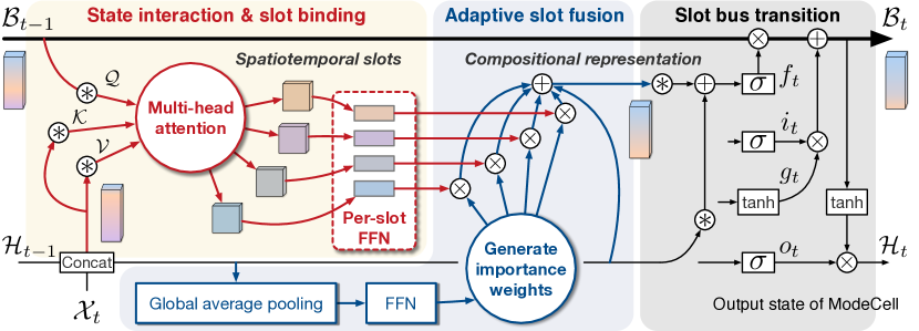
Figure 2: The internal architecture of ModeCell, which is the basic unit in the proposed ModeRNN.

To answer the above questions, we introduce a novel recurrent unit named ModeCell. It follows a decoupling-aggregation framework (see Figure 2) to learn structured hidden representations based on the spatiotemporal slots. Notably, such a framework in the spatiotemporal slot space is completely different from the existing predictive networks with modular architectures (Goyal et al., 2021; Xu et al., 2019). In ModeCell, the spatiotemporal slots are processed in three stages:

• State interaction and slot binding: We first enable the slot bus to interact with the input state and the previous hidden state of ModeRNN through multi-head attention, which naturally improves the decoupling of mixed visual dynamics by dividing output subspaces. To further improves the feature diversity over slots, we then use a feed-forward network (FFN) for each slot to bind the features to independent parameters per slot.

• Adaptive slot fusion: We learn to generate importance weights for the decoupled features in each slot, and obtain compositional representations that explicitly consider the co-existence of multiple patterns in a single sequence. The design of this module meets our key argument: on one hand, different modes from the same data domain should share the same set of key factors of spatiotemporal variations; On the other hand, they are encouraged to differ greatly in the combination of these key factors (corresponding to the slots/patterns above).

• Slot bus transition: We finally update the slot bus using the compositional representations based on spatiotemporal slots, and then generate the output state of ModeCell. Specifically, we use the LSTM-style gated architectures for the slot bus transitions.

Next, we give formalized descriptions of each processing stage in ModeCell.

State interaction and slot binding.

Multi-head attention (Vaswani et al., 2017) is widely used in neural language and image processing, and in this work, it is incorporated in the state transitions of ModeRNN. This mechanism allows interactions between the previous slot bus $\mathcal{B}_{t-1}$, the current input state $\mathcal{X}_{t}$, and the previous hidden state $\mathcal{H}_{t-1}$ (see Figure 2). Formally, at each time step, we first apply 2D convolution projections to $\mathcal{B}_{t-1}$. We then flatten the result to 1D and split it into $N$ spatiotemporal slots along the channel dimension, such that $\{\textrm{slot}_{t-1}^{1},\cdots,\textrm{slot}_{t-1}^{N}\}=\textrm{Split}\left(\textrm{Reshape}\left(W_{q}\ast\mathcal{B}_{t-1}\right)\right)$. Note that $\mathcal{B}_{t-1}\in\mathbb{R}^{H\times W\times(d_{x}+d_{h})}$ and $\textrm{slot}_{t-1}^{n}\in\mathbb{R}^{HW(d_{x}+d_{h})/N}$, where $d_{x}$ is the channel number of input state, $d_{h}$ is that of hidden state, and $H\times W$ indicates the spatial resolution of the slot bus tensor. To improve efficiency, we use two $3\times 3$ depth-wise separable convolutions (Chollet, 2017) for $W_{q}$. We use $\{\textrm{slot}_{t-1}^{1},\cdots,\textrm{slot}_{t-1}^{N}\}$ as the queries of multi-head attention, and apply similar operations to obtain keys $\{\mathcal{K}^{1}_{t},\cdots,\mathcal{K}^{N}_{t}\}$ and values $\{\mathcal{V}^{1}_{t},\cdots,\mathcal{V}^{N}_{t}\}$ based on the concatenation of input state and hidden state, $I_{t}=[\mathcal{X}_{t},\mathcal{H}_{t-1}]$. We then perform multi-head attention and reshape the $N$ output slot features back to 3D tensors:

$$\textrm{slot}_{t}^{n}=\textrm{Reshape}\left(\textrm{softmax}\left(\frac{\textrm{slot}_{t-1}^{n}\cdot{\mathcal{K}_{t}^{n}}^{T}}{\sqrt{d_{k}}}\right)\mathcal{V}_{t}^{n}\right),\ n\in\{1,\cdots,N\},\\$$ (1)

where $d_{k}$ is the dimensionality of the key vectors used as a scaling factor.

Multi-head attention brings two benefits to the forward modeling of spatiotemporal data. First, since $\mathcal{B}_{t-1}$ can be unrolled along the recurrent state transition path to be represented as the transformation of slot features at the previous time step, using $\mathcal{B}_{t-1}$ as attention queries allows the model to extract features from $\mathcal{X}_{t}$ and $\mathcal{H}_{t-1}$ by jointly attending to prior information at different slots. Second, the architecture with $N$ attention heads can naturally help factorize the hidden representation into $N$ subspaces, corresponding to $N$ slots.

After the attention module, each slot representation is then independently modeled using per-slot convolutional layers. We update the slot features by

$$\textrm{slot}_{t}^{n}=\textrm{FFN}_{\textrm{bind}}^{n}\left(\textrm{slot}_{t}^{n}\right),\ n\in\{1,\cdots,N\}.\\$$ (2)

Through random parameter initialization and stochastic gradient descent, the independent networks $\{\textrm{FFN}_{\textrm{bind}}^{1},\cdots,\textrm{FFN}_{\textrm{bind}}^{N}\}$ would most likely be optimized into parameter subspaces far from each other, thus forcing the slots to bind to various components of mixed visual dynamics.

Adaptive slot fusion.

We are motivated by the assumption that different spatiotemporal modes from the same data domain share the same set of slots, and their differences are mainly reflected in the compositional representation based on slot features. Therefore, we propose to dynamically aggregate $\{\textrm{slot}_{t}^{1},\cdots,\textrm{slot}_{t}^{N}\}$ with learnable importance weights assigned to each slot. As shown in Figure 2, we first use the global average pooling (GAP) to compress the contextual information in spacetime from $I_{t}$ to 1D, such that $\textrm{GAP}\left(I_{t}\right)=\frac{1}{H\times W}\sum_{i=1}^{H}\sum_{j=1}^{W}I_{t}(i,j)$. We then use a feed-forward network with a simple fully-connected layer to reduce the dimensionality and get compact representations. Next, we use another group of one-layer fully-connected networks $\{\textrm{FFN}_{\textrm{fuse}}^{1},\cdots,\textrm{FFN}_{\textrm{fuse}}^{N}\}$ with independent parameters to generate $N$ sets of importance weights, such that

$$\omega_{t}^{n}=\textrm{FFN}_{\textrm{fuse}}^{n}\left(\textrm{GAP}\left(I_{t}\right)\right),\ n\in\{1,\cdots,N\}.\\$$ (3)

We further use a residual connection from $I_{t}$ to reduce gradient vanishing, and generate compositional representations $\mathcal{F}_{t}$ based on the learned importance weights and corresponding slot features:

$$\begin{split}\mathcal{F}_{t}&=\textrm{AdaFuse}\left(I_{t},\textrm{slot}_{t}^{1},\cdots,\textrm{slot}_{t}^{N}\right)\\ &=\sigma\left(I_{t}\right)\cdot\left(W_{\textrm{fuse}}^{0}\ast I_{t}\right)+\sum_{n=1}^{N}\sigma(\omega_{t}^{n}\cdot I_{t})\cdot\left(W_{\textrm{fuse}}^{n}\ast\textrm{slot}_{t}^{n}\right),\end{split}$$ (4)

where $\sigma$ denotes the Sigmoid activation function. $W_{\textrm{fuse}}^{\ast}$ is a group of $3\times 3$ convolutional filters.

Slot bus transition.

The compositional representation $\mathcal{F}_{t}$ controls the significance of each slot subspace for a certain sequence at a certain time step. We use four sets of $\mathcal{F}_{t}$ to form the input gate $i_{t}$, forget gate $f_{t}$, output gate $o_{t}$, and input modulation gate $g_{t}$, following the gated recurrent transition mechanism from the standard LSTM. For example, we have $f_{t}=\sigma\left(W_{ff}\ast\mathcal{F}_{t}+W_{fi}\ast\textrm{I}_{t}\right)$ . Finally, we update the state of slot bus and the output state of ModeCell:

$$\begin{split}&\mathcal{B}_{t}=f_{t}\odot\mathcal{B}_{t-1}+i_{t}\odot g_{t}\\ &\mathcal{H}_{t}=o_{t}\odot\tanh(\mathcal{B}_{t}).\\ \end{split}$$ (5)

In terms of network architecture, there are multiple ModeCells stacking in ModeRNN. By analogy, the proposed ModeCell is to ModeRNN what LSTM is to the stacked LSTM network.

4 Experiment

We use three datasets that are commonly used by previous literature to evaluate ModeRNN.

• Mixed Moving MNIST: It consists of three subsets with $1$–$3$ flying digits, corresponding to three spatiotemporal modes obviously reflected in different frequencies of occlusions. Each subset contains $10{,}000$ training sequences and $3{,}000$ testing sequences. We randomly mix each mode’s training sequences, validation sequences, and test sequences to form the overall training, validation, and test sets. Each sequence consists of $20$ consecutive frames, $10$ for input, and $10$ for prediction, in the resolution of $64\times 64$.

• KTH action: The KTH (Schuldt et al., 2004) contains $6$ action categories and involves $25$ subjects in $4$ different scenarios. It thus naturally contains various modes responding to similar action dynamics. We use person $1$-$16$ for training and $17$-$25$ for testing, resize each frame to the resolution of $128\times 128$, and predict $20$ frames from $10$ observations.

• Radar echo: This dataset contains $30{,}000$ sequences of radar echo maps for training, and $3{,}769$ for testing. It naturally contains multiple spatiotemporal modes due to seasonal climate (see Appendix A). Models are trained to predict the next $10$ radar echoes based on the previous $10$ observations. All frames are resized to the resolution of $384\times 384$.

Notably, we do not use any labels in all experiments, because in real-world scenarios, the modes are learned and cannot be pre-defined. In other words, the models are trained in a fully unsupervised way. We train the models with the $L_{2}$ loss, and use the ADAM optimizer (Kingma & Ba, 2015) with a starting learning rate of $0.0003$. The batch size is set to $8$, and the training process is stopped after $80{,}000$ iterations. All experiments are implemented in PyTorch (Paszke et al., 2019) and conducted on NVIDIA TITAN-RTX GPUs. We run all experiments three times and use the average results for quantitative evaluation. Typically, we use $4\times 64$-channel stacked recurrent units in most RNN-based compared models, including ConvLSTM, PredRNN, Conv-TT-LSTM, and ModeRNN

4.1 Demonstration of Spatiotemporal Mode Collapse

We conduct four experiments to explain spatiotemporal mode collapse: (1) t-SNE visualization of learned features, (2) A-distances of learned features corresponding to different modes, (3) quantitative results of models trained on subsets of pre-defined modes, and (4) showcases of prediction results.

t-SNE

In Figure 3(a), we visualize the memory state $\mathcal{C}_{t}$ of ConvLSTM using t-SNE (Van der Maaten & Hinton, 2008)., and find that they are entangled under different digit modes in the Mixed Moving MNIST dataset. It provides evidence that this widely used predictive model cannot learn mode structures effectively. Training the model on a dataset with mixed dynamics leads to severe mode collapse in feature learning, resulting in the entanglement of hidden representations.

A-distance.

A-distance (Ben-David et al., 2010) is defined as $d_{A}=2(1-2\epsilon)$ where $\epsilon$ is the error rate of a domain classifier trained to discriminate two visual domains. In Figure 3(b), we use the A-distance to quantify the spatiotemporal mode collapse in the real-world KTH action dataset. Note that, in this experiment, we divide the KTH dataset into two modes according to the visual similarities of human actions (see details in Appendix B.1). As shown by the blue bars (higher is better), the lower A-distance between the two modes indicates that the learned representations from the two modes are highly entangled. The red bars (lower is better) show the domain distance between features taking as inputs the ground truth frames $\mathcal{X}_{t}$ and those taking the predictions $\widehat{\mathcal{X}}_{t}$. Spatiotemporal mode collapse happens when the A-distance between predictions of different modes (in blue) becomes much smaller than that between predictions and ground truth (in red). We here use the memory state $\mathcal{C}_{t}$ in ConvLSTM and PredRNN, and the slot bus $\mathcal{B}_{t}$ in ModeRNN to calculate A-distance.

Quantitative comparisons of models trained on subset/entire dataset.

To assess spatiotemporal mode collapse, we separately train predictive models on the subsets of Mixed Moving MNIST (with $1$, $2$, and $3$ digits respectively), and then compare the results with that of the model trained on the mixed dataset. As shown in Table 1, previous methods degenerate drastically when using all training samples with mixed visual dynamics. The quantitative results perfectly match the visualization in Figure 3(a), where the features of Mode-2 and Mode-3 are especially entangled and may influence the learning process of each other.

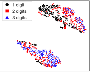
(a) t-SNE on Mixed Moving MNIST

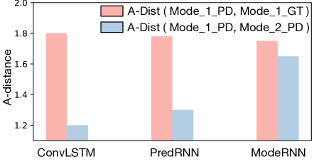
(b) A-distance on KTH

Figure 3: Demonstration of spatiotemporal mode collapse.

Showcases of prediction results.

As shown in Figure 4, we can see that even for the simple case with only $1$ digit, the predicted digit “5” from ConvLSTM is gradually twisted across time and even turns into digit “6” at last. Note that the model is trained on the entire dataset with a variable number of flying digits. The twisted prediction results are caused by the co-existence of the multiple spatiotemporal modes and mode collapse. In the second showcase in Figure 4, the digit “5” is even vanished in the predictions of ConvLSTM (indicated by the red box), showing that the 3-digit prediction is collapse to the 2-digit mode.

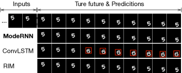
(a) $1$ digit.

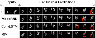
(b) $3$ digits.

Figure 4: Prediction results on the Mixed Moving MNIST dataset.

Table 1: Quantitative results of models for each pre-defined mode. We report results by models learned on sub/entire dataset. Red text indicates improvement by training with entire modes. Green text indicates performance degradation caused by mode collapse.

Model	Mode-1 (1 digit)		Mode-2 (2 digits)		Mode-3 (3 digits)
	SSIM ($\uparrow$)	MSE ($\downarrow$)	SSIM ($\uparrow$)	MSE ($\downarrow$)	SSIM ($\uparrow$)	MSE ($\downarrow$)
ConvLSTM	0.937 / 0.922	26.6 / 33.4	0.848 / 0.839	63.2 / 65.6	0.764 / 0.748	120.5 / 137.1
RIM	0.943 / 0.939	23.4 / 25.3	0.871 / 0.880	53.3 / 52.1	0.814 / 0.803	88.6 / 95.1
ModeRNN	0.946 / 0.951	21.9 / 17.1	0.880 / 0.902	51.0 / 42.1	0.821 / 0.842	83.1 / 74.8

4.2 Visualization of Representations Learned by ModeRNN

To testify the mode decoupling ability of our ModeRNN, we visualize the slot features in Figure 5(a). Here, we use $4$ spatiotemporal slots. We can see that these slot features are obviously clustered into exact $4$ groups, indicating that different slots of ModeRNN learn diverse dynamic patterns from highly mixed spatiotemporal modes. In Figure 5(b), we further visualize the features in the slot bus, which show $3$ clusters with clear boundaries, corresponding to the three modes with different numbers of digits. In Figure 5(c), we visualize the importance weights of samples in different modes. The above results indicate that, first, the spatiotemporal slots are successfully bound to different components of visual dynamics; Second, the compositional representations based on the slots, including the slot but, successfully learn discriminative knowledge from different dynamic modes.

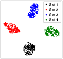
(a) Spatiotemporal slots

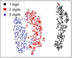
(b) Slot bus

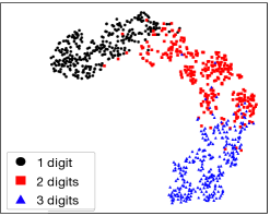
(c) Importance weights

Figure 5: Visualization of representations learned by ModeRNN on the Mixed Moving MNIST.

4.3 Resuls of ModeRNN on Mixed Moving MNIST

Main results.

Table 1 gives the results on each subset of flying digit mode. We can see that only ModeRNN achieves consistently better performance on each mode. It is also the only one that can consistently benefit from training with mixed dynamics from the entire dataset. Besides, in Table 2, we show the overall quantitative results as well as computational efficiency of the compared models on the Mixed Moving MNIST dataset. As we can see, ModeRNN achieves state-of-the-art overall performance (SSIM: 0.897, MSE: 44.7) with fewer parameters compared with existing approaches, including the more recent work (Goyal et al., 2021) also with modular architectures. Furthermore, as shown in Figure 4, ModeRNN is the only method that can capture the exact movement of each digit, while other models predict the blurry results and the digit “5” is even vanished. All in all, our ModeRNN could effectively overcome the spatiotemporal mode collapse to achieve competitive performance on complex datasets.

Hyperparameters analysis on the number of slots.

In Table 3, we gradually increase the number of spatiotemporal slots from $1$, finding that the performance of ModeRNN increases rapidly at the early stage and achieves the best performance on $N=4$. We have similar results on all benchmarks and set $N=4$ throughout this paper.

Ablation study on model components.

We analyze the efficacy of each network component in ModeRNN on the Mixed Moving MNIST dataset, as shown in Table 4. Without the adaptive slot fusion module, the model can not work well by simply adding different slot features with equal weights (MSE: 44.7 → 60.5), which strongly demonstrates that learning adaptive, compositional representations over the slot features is crucial to modeling the underlying structure of visual dynamics and can therefore better decouple the learned spatiotemporal modes.

Table 2: Quantitative results and parameter analysis on the Mixed Moving MNIST dataset. Here, we report the training time for $1{,}000$ sequences.

Model	SSIM ($\uparrow$)	MSE ($\downarrow$)	Param (MB)	Time (s)	Mem (GB)
ConvLSTM (Shi et al., 2015)	0.836	78.7	8.15	29	2.58
PredRNN (Wang et al., 2017)	0.851	67.3	11.83	68	3.52
MIM (Wang et al., 2019b)	0.851	64.4	18.45	73	4.22
Conv-TT-LSTM (Su et al., 2020)	0.866	61.2	7.58	77	6.17
RIM (Goyal et al., 2021)	0.874	57.5	7.91	71	5.88
ModeRNN	0.898	44.7	6.35	59	3.15

Table 3: The ablation study of ModeRNN with respect to the number of spatiotemporal slots.

Model	Per-frame MSE
ModeRNN ($N=1$)	69.3
ModeRNN ($N=2$)	59.4
ModeRNN ($N=3$)	48.2
ModeRNN ($N=4$, final proposed)	44.7
ModeRNN ($N=5$)	45.9

Table 4: The ablation study on the adaptive slot fusion module and the slot binding module on the mixed Moving MNIST dataset.

Model	Per-frame MSE
ModeRNN	44.7
ModeRNN w/o Slot Binding ($N=1$)	69.3
ModeRNN w/o Adaptive Slot Fusion	60.5

4.4 Resuls of ModeRNN on the KTH Action Dataset

On this dataset, we use the frame-wise peak signal-to-noise ratio (PSNR) and learned perceptual image patch similarity (LPIPS) (Zhang et al., 2018) as evaluation metrics. In the left column of Table 5, we show the quantitative results of the KTH dataset and find that ModeRNN achieves better overall performance among all compared methods. Impressively, ModeRNN overcomes the mode collapse effectively and achieves better performance compared with the powerful probabilistic model SVG (Denton & Fergus, 2018) (PSNR : 27.73 vs 28.22, LPIPS : 0.196 vs 0.183). We provide the qualitative showcases in Figure 6 where we can see that ModeRNN can predict the precise position of the moving person.

Table 5: Quantitative results on the KTH action dataset and the radar echo dataset. For the probabilistic SVG model, we report the best results from $100$ output samples per input sequence.

Model	KTH		Radar
	PSNR ($\uparrow$)	LPIPS ($\downarrow$)	CSI30 ($\uparrow$)	MSE ($\downarrow$)
ConvLSTM (Shi et al., 2015)	24.12	0.231	0.354	97.6
TrajGRU (Shi et al., 2017)	26.97	0.219	0.357	89.2
PredRNN (Wang et al., 2017)	27.47	0.212	0.359	84.2
SVG (Denton & Fergus, 2018)	27.73	0.196	-	-
Conv-TT-LSTM (Su et al., 2020)	27.59	0.198	0.363	87.6
ModeRNN	28.22	0.183	0.428	65.1

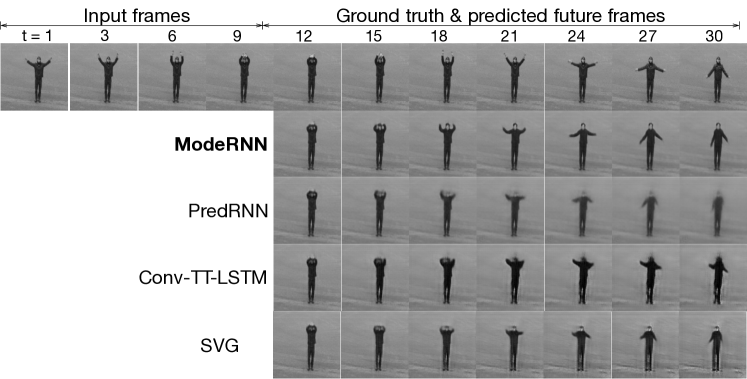
Figure 6: Prediction frames on the KTH action dataset.

4.5 Resuls of ModeRNN on the Radar Echo Dataset

Besides the frame-wise MSE, we use the Critical Success Index (CSI) metric, which is defined as $\textrm{CSI}=\frac{\textrm{Hits}}{\textrm{Hits}+\textrm{Misses}+\textrm{FalseAlarms}}$, where hits correspond to the true positive, misses correspond to the false positive, and false alarms correspond to the false negative. A higher CSI indicates better forecasting performance, and it is particularly sensitive to high-intensity echoes. We set the alarm threshold to $30$ dBZ for this radar benchmark. As shown in the right column of Table 5, ModeRNN achieves the state-of-the-art overall performance and significantly outperforms the competitive precipitation method, TrajGRU (Shi et al., 2017) (CSI: 0.428 vs 0.357, MSE: 65.1 vs 89.2).

As shown in Figure 7, we find that the compared models fail in predicting the edges of the cyclone, and the predicted movement of the cloud even vanishes. On the contrary, ModeRNN provides more details for the cyclone and accurately predicts its center position indicated by the red box. Both the quantitative and qualitative results show that our ModeRNN can effectively capture the dynamic information from complex meteorological dynamic modes.

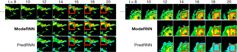
Figure 7: Prediction results on the radar echo dataset.

5 Conclusion

In this paper, we demonstrated a new experimental phenomenon of spatiotemporal mode collapse when training unsupervised predictive models on a dataset with highly mixed visual dynamics. Accordingly, we proposed a novel predictive network named ModeRNN, which can effectively learn modular features from the mixed dataset using a set of spatiotemporal slots. To discover the compositional structures in spatiotemporal modes, ModeRNN adaptively aggregates the slot features with learnable importance weight. Compared with existing models, ModeRNN was shown to prevent the mode collapse of future predictions in spacetime, improving qualitative and quantitative results on three widely used datasets.

Appendix A Illustration of Mixed Modes for Precipitation Forecasting

Real-world spatiotemporal datasets usually contain a variety of latent modes of visual dynamics without human annotations. As discussed in Section 4.5, we take precipitation forecasting based on radar echo observations as a practical application scenario of spatiotemporal prediction. Figure 8 gives an example of the mixed dynamics for the typical climate in Guangzhou, China. Obviously, since the climate changes smoothly between seasons with fuzzy boundaries, it is inappropriate to pre-assign mode labels before forecast.

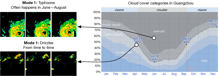
Figure 8: Illustration of mixed spatiotemporal modes in the radar echo dataset. In practice, we cannot pre-assign mode labels before forecast because of the fuzzy boundaries between seasonal climates.

Appendix B Additional Results and Discussion

B.1 Training Models on Subsets Divided by Pre-Defined Mode Labels

Subsets in KTH based on pre-defined action categories.

According to the scale of the actions, we can simply group the existing six categories in the KTH dataset into two typical modes:

• The first mode corresponds to the global movement of the torso, including the categories of running, walking, and jogging.

• The second mode corresponds to the local movement of hands, including the categories of hand clapping, hand waving, and boxing.

Table 6: Quantitative results of models that are learned on the sub/entire KTH action dataset. For the probabilistic SVG model (Denton & Fergus, 2018), we report the best results from $100$ output samples per input sequence.

Model	Mode-1 (torso movement)		Mode-2 (hand movement)		Overall
	PSNR ($\uparrow$)	LPIPS ($\downarrow$)	PSNR ($\uparrow$)	LPIPS ($\downarrow$)	PSNR ($\uparrow$)	LPIPS ($\downarrow$)
Shi et al. (2015)	23.65 / 23.13	0.227 / 0.232	24.37 / 24.98	0.234 / 0.230	24.03 / 24.12	0.231 / 0.231
Wang et al. (2017)	27.45 / 26.92	0.218 / 0.226	27.52 / 27.94	0.203 / 0.199	27.49 / 27.47	0.210 / 0.212
Denton & Fergus (2018)	27.79 / 27.34	0.193 / 0.199	27.75 / 28.12	0.197 / 0.193	27.77 / 27.73	0.195 / 0.196
Su et al. (2020)	27.57 / 27.09	0.192 / 0.204	27.64 / 28.03	0.201 / 0.192	27.61 / 27.59	0.196 / 0.198
ModeRNN	27.84 / 28.11	0.192 / 0.185	27.82 / 28.32	0.196 / 0.181	27.83 / 28.22	0.194 / 0.183

Subsets in the radar echo dataset based on pre-defined chronological climate modes.

Considering the climate change between different seasons in Guangzhou, we can roughly divide the radar echo dataset into two typical meteorology groups:

• The first mode: It corresponds to the windier part of the year, from March to May, with average wind speeds of more than $7.5$ miles per hour. There will be drizzles from time to time in these months. We use the radar maps from $2016/3$ to $2016/5$ and from $2017/3$ to $2017/4$ for training, and use those in $2017/5$ for testing.

• The second mode: It corresponds to the the summer in Guangzhou, which from Figure LABEL:fig:intro, experiences heavier cloud cover, with the percentage of time that the sky is overcast or mostly cloudy is around $80\%$. We use the radar maps from $2016/6$ to $2016/8$ and from $2017/6$ to $2017/7$ for training, and use those in $2017/8$ for testing.

Table 7: Quantitative results of models that are learned on the sub/entire radar echo dataset. Red text indicates improvement by joint training. Green text indicates performance degradation caused by mode collapse.

Model	Mode-1 (Mar.–May)		Mode-2 (Jun.–Aug.)		Overall
	CSI30 ($\uparrow$)	MSE ($\downarrow$)	CSI30 ($\uparrow$)	MSE ($\downarrow$)	CSI30 ($\uparrow$)	MSE ($\downarrow$)
Shi et al. (2015)	0.341 / 0.337	63.5 / 71.3	0.372 / 0.366	102.4 / 116.7	0.359 / 0.354	86.0 / 97.6
Shi et al. (2017)	0.354 / 0.341	62.5 / 68.3	0.375 / 0.369	99.3 / 104.3	0.366 / 0.357	83.8 / 89.2
Wang et al. (2017)	0.357 / 0.342	57.1 / 60.8	0.384 / 0.371	97.5 / 101.2	0.373 / 0.359	80.5 / 84.2
Su et al. (2020)	0.359 / 0.347	61.5 / 65.8	0.381 / 0.374	99.1 / 103.5	0.372 / 0.363	83.3 / 87.6
ModeRNN	0.373 / 0.408	54.3 / 46.2	0.392 / 0.442	92.0 / 78.8	0.384 / 0.428	76.1 / 65.1

References

- Ben-David et al. (2010) Shai Ben-David, John Blitzer, Koby Crammer, Alex Kulesza, Fernando Pereira, and Jennifer Wortman Vaughan. A theory of learning from different domains. Machine Learning, pp. 151–175, 2010.
- Bhagat et al. (2020) Sarthak Bhagat, Shagun Uppal, Zhuyun Yin, and Nengli Lim. Disentangling multiple features in video sequences using gaussian processes in variational autoencoders. In ECCV, pp. 102–117, 2020.
- Castrejon et al. (2019) Lluis Castrejon, Nicolas Ballas, and Aaron Courville. Improved conditional VRNNs for video prediction. In CVPR, pp. 7608–7617, 2019.
- Chollet (2017) François Chollet. Xception: Deep learning with depthwise separable convolutions. In CVPR, pp. 1251–1258, 2017.
- De Brabandere et al. (2016) Bert De Brabandere, Xu Jia, Tinne Tuytelaars, and Luc Van Gool. Dynamic filter networks. In NeurIPS, pp. 667–675, 2016.
- Denton & Fergus (2018) Emily Denton and Rob Fergus. Stochastic video generation with a learned prior. In ICML, pp. 1182–1191, 2018.
- Denton et al. (2017) Emily L Denton et al. Unsupervised learning of disentangled representations from video. In NeurIPS, pp. 4417–4426, 2017.
- Goyal et al. (2021) Anirudh Goyal, Alex Lamb, Jordan Hoffmann, Shagun Sodhani, Sergey Levine, Yoshua Bengio, and Bernhard Schölkopf. Recurrent independent mechanisms. In ICLR, 2021.
- Guen & Thome (2020) Vincent Le Guen and Nicolas Thome. Disentangling physical dynamics from unknown factors for unsupervised video prediction. In CVPR, pp. 11474–11484, 2020.
- Hsieh et al. (2018) Jun-Ting Hsieh, Bingbin Liu, De-An Huang, Li Fei-Fei, and Juan Carlos Niebles. Learning to decompose and disentangle representations for video prediction. In NeurIPS, 2018.
- Kalchbrenner et al. (2017) Nal Kalchbrenner, Aaron van den Oord, Karen Simonyan, Ivo Danihelka, Oriol Vinyals, Alex Graves, and Koray Kavukcuoglu. Video pixel networks. In ICML, pp. 1771–1779, 2017.
- Kingma & Ba (2015) Diederik Kingma and Jimmy Ba. Adam: A method for stochastic optimization. In ICLR, 2015.
- Kwon & Park (2019) Yong-Hoon Kwon and Min-Gyu Park. Predicting future frames using retrospective cycle GAN. In CVPR, pp. 1811–1820, 2019.
- Locatello et al. (2020) Francesco Locatello, Dirk Weissenborn, Thomas Unterthiner, Aravindh Mahendran, Georg Heigold, Jakob Uszkoreit, Alexey Dosovitskiy, and Thomas Kipf. Object-centric learning with slot attention. In NeurIPS, 2020.
- Mathieu et al. (2016) Michael Mathieu, Camille Couprie, and Yann LeCun. Deep multi-scale video prediction beyond mean square error. In ICLR, 2016.
- Oh et al. (2015) Junhyuk Oh, Xiaoxiao Guo, Honglak Lee, Richard L Lewis, and Satinder Singh. Action-conditional video prediction using deep networks in atari games. In NeurIPS, pp. 2863–2871, 2015.
- Oliu et al. (2018) Marc Oliu, Javier Selva, and Sergio Escalera. Folded recurrent neural networks for future video prediction. In ECCV, pp. 716–731, 2018.
- Paszke et al. (2019) Adam Paszke, Sam Gross, Francisco Massa, Adam Lerer, James Bradbury, Gregory Chanan, Trevor Killeen, Zeming Lin, Natalia Gimelshein, Luca Antiga, Alban Desmaison, Andreas Köpf, Edward Yang, Zachary DeVito, Martin Raison, Alykhan Tejani, Sasank Chilamkurthy, Benoit Steiner, Lu Fang, Junjie Bai, and Soumith Chintala. PyTorch: An imperative style, high-performance deep learning library. In NeurIPS, pp. 8024–8035, 2019.
- Ranzato et al. (2014) MarcAurelio Ranzato, Arthur Szlam, Joan Bruna, Michael Mathieu, Ronan Collobert, and Sumit Chopra. Video (language) modeling: a baseline for generative models of natural videos. arXiv preprint arXiv:1412.6604, 2014.
- Schuldt et al. (2004) Christian Schuldt, Ivan Laptev, and Barbara Caputo. Recognizing human actions: a local SVM approach. In ICPR, pp. 32–36, 2004.
- Shi et al. (2015) Xingjian Shi, Zhourong Chen, Hao Wang, Dit-Yan Yeung, Wai-Kin Wong, and Wang-chun Woo. Convolutional LSTM network: A machine learning approach for precipitation nowcasting. In NeurIPS, pp. 802–810, 2015.
- Shi et al. (2017) Xingjian Shi, Zhihan Gao, Leonard Lausen, Hao Wang, Dit-Yan Yeung, Wai-kin Wong, and Wang-chun Woo. Deep learning for precipitation nowcasting: A benchmark and a new model. In NeurIPS, pp. 5617–5627, 2017.
- Srivastava et al. (2015) Nitish Srivastava, Elman Mansimov, and Ruslan Salakhutdinov. Unsupervised learning of video representations using LSTMs. In ICML, pp. 843–852, 2015.
- Su et al. (2020) Jiahao Su, Wonmin Byeon, Furong Huang, Jan Kautz, and Animashree Anandkumar. Convolutional tensor-train lstm for spatio-temporal learning. In NeurIPS, 2020.
- Tulyakov et al. (2018) Sergey Tulyakov, Ming-Yu Liu, Xiaodong Yang, and Jan Kautz. MoCoGAN: Decomposing motion and content for video generation. In CVPR, pp. 1526–1535, 2018.
- Van der Maaten & Hinton (2008) Laurens Van der Maaten and Geoffrey Hinton. Visualizing data using t-sne. Journal of machine learning research, 9(11), 2008.
- Vaswani et al. (2017) Ashish Vaswani, Noam Shazeer, Niki Parmar, Jakob Uszkoreit, Llion Jones, Aidan N Gomez, Lukasz Kaiser, and Illia Polosukhin. Attention is all you need. arXiv preprint arXiv:1706.03762, 2017.
- Villegas et al. (2018) Ruben Villegas, Jimei Yang, Yuliang Zou, Sungryull Sohn, Xunyu Lin, and Honglak Lee. Learning to generate long-term future via hierarchical prediction. In ICML, pp. 3560–3569, 2018.
- Vondrick et al. (2016) Carl Vondrick, Hamed Pirsiavash, and Antonio Torralba. Generating videos with scene dynamics. In NeurIPS, pp. 613–621, 2016.
- Wang et al. (2018) Ting-Chun Wang, Ming-Yu Liu, Jun-Yan Zhu, Guilin Liu, Andrew Tao, Jan Kautz, and Bryan Catanzaro. Video-to-video synthesis. arXiv preprint arXiv:1808.06601, 2018.
- Wang et al. (2017) Yunbo Wang, Mingsheng Long, Jianmin Wang, Zhifeng Gao, and S Yu Philip. PredRNN: Recurrent neural networks for predictive learning using spatiotemporal lstms. In NeurIPS, pp. 879–888, 2017.
- Wang et al. (2019a) Yunbo Wang, Lu Jiang, Ming-Hsuan Yang, Li-Jia Li, Mingsheng Long, and Li. Fei-Fei. Eidetic 3D LSTM: A model for video prediction and beyond. In ICLR, 2019a.
- Wang et al. (2019b) Yunbo Wang, Jianjin Zhang, Hongyu Zhu, Mingsheng Long, Jianmin Wang, and Philip S. Yu. Memory in memory: A predictive neural network for learning higher-order non-stationarity from spatiotemporal dynamics. In CVPR, pp. 9154–9162, 2019b.
- Xu et al. (2018) Jingwei Xu, Bingbing Ni, and Xiaokang Yang. Video prediction via selective sampling. In NeurIPS, pp. 1712–1722, 2018.
- Xu et al. (2019) Zhenjia Xu, Zhijian Liu, Chen Sun, Kevin Murphy, William T Freeman, Joshua B Tenenbaum, and Jiajun Wu. Unsupervised discovery of parts, structure, and dynamics. In ICLR, 2019.
- Yao et al. (2020) Zhiyu Yao, Yunbo Wang, Mingsheng Long, and Jianmin Wang. Unsupervised transfer learning for spatiotemporal predictive networks. In ICML, pp. 10778–10788, 2020.
- Yu et al. (2019) Wei Yu, Yichao Lu, Steve Easterbrook, and Sanja Fidler. Efficient and information-preserving future frame prediction and beyond. In ICLR, 2019.
- Zhang et al. (2018) Richard Zhang, Phillip Isola, Alexei A Efros, Eli Shechtman, and Oliver Wang. The unreasonable effectiveness of deep features as a perceptual metric. In CVPR, pp. 586–595, 2018.