Unsupervised Cross-Lingual Transfer of Structured Predictors
without Source Data

Abstract

Providing technologies to communities or domains where training data is scarce or protected e.g., for privacy reasons, is becoming increasingly important. To that end, we generalise methods for unsupervised transfer from multiple input models for structured prediction. We show that the means of aggregating over the input models is critical, and that multiplying marginal probabilities of substructures to obtain high-probability structures for distant supervision is substantially better than taking the union of such structures over the input models, as done in prior work. Testing on 18 languages, we demonstrate that the method works in a cross-lingual setting, considering both dependency parsing and part-of-speech structured prediction problems. Our analyses show that the proposed method produces less noisy labels for the distant supervision.

Introduction

Recent successes of artificial intelligence (AI) systems have been enabled by supervised learning algorithms that require a large amount of human-labelled data. Such data is costly to create, and it can be prohibitively expensive for structured prediction tasks such as dependency parsing (Böhmová et al. 2003; Brants, Skut, and Uszkoreit 2003). Transfer learning (Pan and Yang 2010) is a promising solution to facilitate the development of AI systems on a domain without such data. In this work, we focus on a particular case of transfer learning, namely cross-lingual learning, which seeks to transfer across languages. We consider the setup where the target language is low-resource having only unlabelled data, commonly referred to as unsupervised cross-lingual transfer. This is an important problem because most world’s languages are low-resource (Joshi et al. 2020). Successful transfer from high-resource languages enables language technologies development for these low-resource languages.

One recent method for unsupervised cross-lingual transfer is PPTX (Kurniawan et al. 2021). It is developed for dependency parsing and allows transfer from multiple source languages, which has been shown to be generally superior to transferring from just a single language (McDonald, Petrov, and Hall 2011; Duong et al. 2015; Rahimi, Li, and Cohn 2019, inter alia). An advantage of PPTX is that, in addition to not requiring any labelled data in the target language, it does not require access to any data in the source languages either, which is useful if the source data is private. All it needs is access to multiple, trained source parsers. Despite its benefits, PPTX has only been applied to dependency parsing, although in principle it should be extensible to other structured prediction problems. More concerningly, we show in this work that PPTX generally underperforms compared to a multi-source transfer baseline based on majority voting.

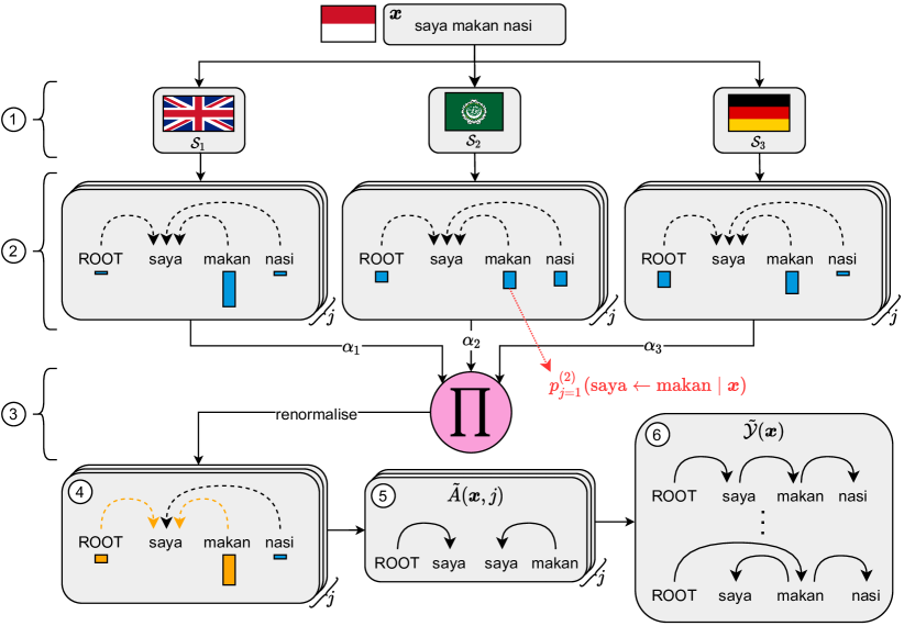
Figure 1: Illustration of our method for an input sentence saya makan nasi (“I eat rice”). 1 A set of structured prediction models as inputs. 2 The models compute marginal probability distributions over substructures for each token $x_{j}$. 3 Logarithmic opinion pool of the distributions is computed. 4 Substructures are filtered based on some threshold. 5 High-probability substructures are obtained. 6 High-probability structures are obtained from the substructures as distant supervision.

In this paper, we generalise and improve PPTX by reformulating it for structured prediction problems. As with PPTX, this generalisation casts the unsupervised transfer problem as a supervised learning task with distant supervision, where the label of each sample in the target language is based on the structures predicted by an ensemble of source models. Moreover, we propose the use of logarithmic opinion pooling (Heskes 1998) to improve performance (see Fig. 1). Unlike PPTX that performs simple union, the pooling considers the output probabilities in aggregating the source model outputs to obtain the structures used for distant supervision. We test our method on 18 languages from 5 language families and on two structured prediction tasks in NLP: dependency parsing and part-of-speech tagging. We find that our method generally outperforms both PPTX and the majority voting baseline, with absolute accuracy gains of up to $7\text{\,}\mathrm{\char 37\relax}$ on parsing and $20\text{\,}\mathrm{\char 37\relax}$ on tagging. Our analysis shows that the use of logarithmic opinion pooling results in fewer predicted structures that are also more concentrated on the correct ones.

In summary, our contributions in this paper are:

• developing a generic unsupervised multi-source transfer method for structured prediction problems;

• leveraging logarithmic opinion pooling to take into account source model probabilities in the aggregation to produce the labels for distant supervision; and

• outperforming previous work in dependency parsing and part-of-speech tagging, especially in the context of a stronger, multi-source transfer baseline.

Unsupervised Transfer as Supervised Learning

Suppose we want to create a model for a low-resource language that has only unlabelled data, but we only have access to a set of models trained on other languages. This is an instance of cross-lingual transfer learning. We cast this problem as a (distantly) supervised learning task with the training objective

$$\ell(\boldsymbol{\theta})=-\sum_{\boldsymbol{x}\in\mathcal{D}}\log\sum_{\boldsymbol{y}\in\tilde{\mathcal{Y}}(\boldsymbol{x})}p(\boldsymbol{y}\mid\boldsymbol{x};\boldsymbol{\theta})$$ (1)

where $\boldsymbol{\theta}$ is the target model parameters, $\mathcal{D}$ is the unlabelled target data, and $\tilde{\mathcal{Y}}(\boldsymbol{x})$ is a set of distant supervision labels for an unlabelled input $\boldsymbol{x}=x_{1}x_{2}\cdots x_{n}$. Thus, $\tilde{\mathcal{Y}}(\boldsymbol{x})$ contains supervision in the form of one or more potentially ambiguous/uncertain labels. In single-source transfer, $\tilde{\mathcal{Y}}(\boldsymbol{x})$ can be as simple as a singleton containing the predicted label for $\boldsymbol{x}$ by the source model, in which case this is related to self-training (McClosky, Charniak, and Johnson 2006). In our case, however, this supervision is assumed to arise from an ensemble of models, each is based on transfer from a different source language (see next section). The parameters $\boldsymbol{\theta}$ can be initialised to the source model parameters and regularised to this initialiser during training, in order to both speed up training and encourage the parameters to stay near known good parameter values. Overall, the objective becomes $\ell^{\prime}(\boldsymbol{\theta})=\ell(\boldsymbol{\theta})+\lambda\lVert\boldsymbol{\theta}-\boldsymbol{\theta}_{0}\rVert^{2}_{2}$ where $\boldsymbol{\theta}_{0}$ is the source model parameters and $\lambda$ is a hyperparameter controlling the regularisation strength.

Supervision via Ensemble

In multi-source transfer, the set $\tilde{\mathcal{Y}}(\boldsymbol{x})$ can be obtained by an ensemble method applied to the source models. PPTX (Kurniawan et al. 2021) is one such method designed for arc-factored dependency parsers. We generalise PPTX, making it applicable to any set of source models that predict structured outputs that decompose into substructures (of which a set of arc-factored dependency parsers is a special case). For the rest of this paper, we assume that the source models are graphical models over these structured outputs. Let $C(\boldsymbol{x},j)$ denote the set of substructures associated with $x_{j}$ whose marginal probabilities form a probability distribution:

$$\sum_{c\in C(\boldsymbol{x},j)}p^{(k)}(c\mid\boldsymbol{x})=1$$ (2)

for any source model $k$. For example, for dependency parsing, $C(\boldsymbol{x},j)$ is the set of arcs whose dependent is $x_{j}$ (see Fig. 1 part 2). The chart $\tilde{\mathcal{Y}}(\boldsymbol{x})$ can then be obtained as follows. Define $\tilde{A}_{k}(\boldsymbol{x},j)$ to be the set of substructures associated with $x_{j}$ having high marginal probability under source model $k$. This set is obtained by adding substructures $c\in C(\boldsymbol{x},j)$ in descending order of their marginal probability until their cumulative probability exceeds a threshold $\sigma$:

$$\sum_{c\in C(\boldsymbol{x},j)}p^{(k)}(c\mid\boldsymbol{x})\geq\sigma$$ (3)

where $0\leq\sigma\leq 1$. Therefore, $\tilde{A}_{k}(\boldsymbol{x},j)$ contains the substructures that cover at least $\sigma$ probability mass of the output space under source model $k$. Next, define

$$\tilde{A}(\boldsymbol{x})=\bigcup_{k,j}\tilde{A}_{k}(\boldsymbol{x},j)$$ (4)

as the set of high probability substructures for $\boldsymbol{x}$ given by the source models. The chart $\tilde{\mathcal{Y}}(\boldsymbol{x})$ is then defined as the set of structures whose substructures are all in $\tilde{A}(\boldsymbol{x})$. Formally,

$$\tilde{\mathcal{Y}}(\boldsymbol{x})=\{\boldsymbol{y}\mid\boldsymbol{y}\in\mathcal{Y}(\boldsymbol{x})\wedge A(\boldsymbol{y})\subseteq\tilde{A}(\boldsymbol{x})\}$$ (5)

where $\mathcal{Y}(\boldsymbol{x})$ is the output space of $\boldsymbol{x}$ and $A(\boldsymbol{y})$ is the set of substructures in $\boldsymbol{y}$. To prevent $\tilde{\mathcal{Y}}(\boldsymbol{x})$ from being empty, the 1-best structure $\hat{\boldsymbol{y}}=\arg\max_{\boldsymbol{y}}p^{(k)}(\boldsymbol{y}\mid\boldsymbol{x})$ from each source model $k$ is also included in the chart, but they don’t count toward the probability threshold.

Proposed Method

Multilinguality is the key factor contributing to the success of PPTX (Kurniawan et al. 2021). Therefore, optimising the method to leverage this multilinguality provided by the source models is important. One potential limitation of PPTX is the inclusion of substructures having relatively low marginal probability under some source model because of the union in Eq. 4. As an extreme illustration, consider a poor source model $k$ assigning uniform marginal probability to substructures in $C(\boldsymbol{x},j)$. Most of these substructures will be included in $\tilde{A}_{k}(\boldsymbol{x},j)$ and, subsequently, $\tilde{A}(\boldsymbol{x})$. As a result, noisy structures may be included in $\tilde{\mathcal{Y}}(\boldsymbol{x})$ which makes learning the correct structure difficult.

Instead of computing the set of high-probability substructures from each source model separately, a potentially better alternative is to aggregate the marginal probabilities given by the source models and then compute the chart from the resulting distribution. We propose to use logarithmic opinion pooling (Heskes 1998) as the aggregation method. To obtain the chart $\tilde{\mathcal{Y}}(\boldsymbol{x})$, first we compute the logarithmic opinion pool of the source models’ marginal probabilities. That is, for all $j\in\{1,\ldots,n\}$, define

$$\bar{p}_{j}(c\mid\boldsymbol{x})\propto\prod_{k}\left[p^{(k)}(c\mid\boldsymbol{x})\right]^{\alpha_{k}}$$ (6)

where we normalise over the substructures $c\in C(\boldsymbol{x},j)$, and $\alpha_{k}$ is a non-negative scalar weighting the contribution of source model $k$ satisfying $\sum_{k}\alpha_{k}=1$. Thus, $\bar{p}_{j}$ gives the new probability distribution over substructures in $C(\boldsymbol{x},j)$. Then, we compute the set $\tilde{A}(\boldsymbol{x},j)$ using $\bar{p}_{j}$ in a similar fashion as before: adding substructures $c\in C(\boldsymbol{x},j)$ in descending order by their marginal probability given by $\bar{p}_{j}$ until their cumulative probability exceeds $\sigma$. Lastly, we define $\tilde{A}(\boldsymbol{x})=\bigcup_{j}\tilde{A}(\boldsymbol{x},j)$, and keep the definition of $\tilde{\mathcal{Y}}(\boldsymbol{x})$ unchanged: the set of structures induced by $\tilde{A}(\boldsymbol{x})$ plus the 1-best structures, which is used as labels for training with the objective in Eq. 1. Fig. 1 illustrates the process using dependency parsing as an example.

Setting the Weight Factors

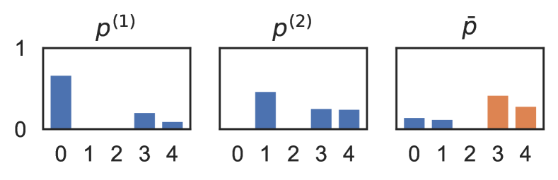
Figure 2: Logarithmic opinion pool with uniform weighting ($\bar{p}$) for two distributions $p^{(1)}$ and $p^{(2)}$. The opinion pool $\bar{p}$ assigns lower probabilities to substructures indexed by 0 and 1 than those indexed by 3 and 4 because $p^{(1)}$ and $p^{(2)}$ assign very low probability to either 0 or 1. Selected substructures in the context of Eq. 3 with $\sigma=0.7$ are in orange.

Finding an optimal value for $\alpha_{k}$ is possible if there is labelled data (Heskes 1998). However, we do not have labelled data in the target language in our cross-lingual setup. There is some method to find similar weighting scalars for cross-lingual transfer that may work in our setup (Wu et al. 2020), but they assume access to unlabelled source language data and only marginally outperform uniform weighting. Therefore, unless stated otherwise, we set $\alpha_{k}$ uniformly, reducing Eq. 6 to the normalised geometric mean of the marginal distributions.

Motivation

The motivation behind the proposed method is the observation that PPTX obtains the high-probability substructures by applying the threshold in Eq. 3 for each source model separately before they are aggregated into a single set in Eq. 4. This means PPTX “trusts” all source models equally regardless of their certainty about their predictions. In contrast, our method takes into account the probabilities given by the source models by applying the threshold after aggregating the probabilities in the logarithmic opinion pool in Eq. 6. The opinion pool assigns more probability mass to substructures to which all the source models assign a high probability (see Fig. 2), and we hypothesise that such substructures are more likely to be correct.

Application to Structured Prediction

The above method can be applied to structured prediction problems. Crucial to the application is the definition of $C(\boldsymbol{x},j)$. Below, we present two applications: arc-factored dependency parsing and sequence tagging.

Arc-Factored Dependency Parsing

For dependency parsing, we can define $C(\boldsymbol{x},j)$ as the set of dependency arcs having $x_{j}$ as dependent:

$$C(\boldsymbol{x},j)=\{(i,j,l)\mid i\in\{0,1,\ldots,n\}\wedge i\neq j\wedge l\in L\}$$ (7)

where $(i,j,l)$ denotes an arc from head $x_{i}$ to dependent $x_{j}$ with dependency label $l$, $L$ denotes the set of dependency labels, and $x_{0}$ is a special token whose dependent is the root of the sentence. Since exactly one arc in $C(\boldsymbol{x},j)$ exists in any possible dependency tree of $\boldsymbol{x}$, the marginal probabilities of arcs in $C(\boldsymbol{x},j)$ form a probability distribution. The rest follows accordingly. The set $\tilde{A}_{k}(\boldsymbol{x},j)$ becomes the set of arcs with $x_{j}$ as dependent that have high marginal probability under source model $k$. The set $\tilde{A}(\boldsymbol{x})$ becomes the set of high probability arcs for the whole sentence. Lastly, the chart $\tilde{\mathcal{Y}}(\boldsymbol{x})$ contains all possible trees for $\boldsymbol{x}$ whose arcs are all in $\tilde{A}(\boldsymbol{x})$. The predicted tree from each source parser is included in the chart as well.

Sequence Tagging

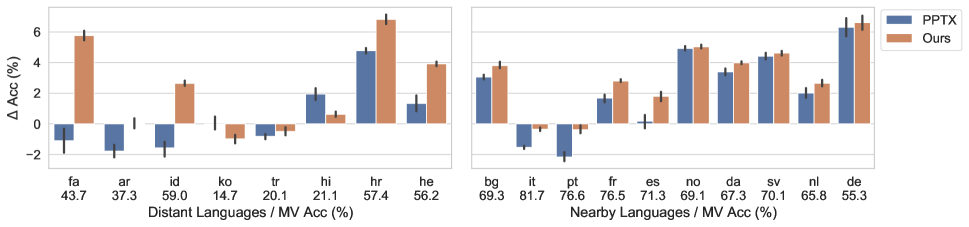
(a) Dependency parsing

(b) POS tagging

Figure 3: Performance difference of PPTX and our method against the majority voting baseline on dependency parsing and POS tagging. Numbers below the language label are the majority voting baseline performance, which corresponds to the zero value on the y-axis.

In sequence tagging, the structured output is a sequence of tags, which decomposes into consecutive tag pairs. Given a sequence of tags $\boldsymbol{y}=y_{1}y_{2}\cdots y_{n}$ corresponding to the input $\boldsymbol{x}$, its consecutive tag pairs are $A(\boldsymbol{y})=\{(j,y_{j},y_{j+1})\}_{j=1}^{n-1}$. We define $C(\boldsymbol{x},j)$ as the set of possible tag pairs for $x_{j}$ and $x_{j+1}$:

$$C(\boldsymbol{x},j)=\{(j,t,t^{\prime})\mid(t,t^{\prime})\in T\times T\}$$ (8)

where $T$ is the set of tags. Note that any sequence of tags for $\boldsymbol{x}$ has exactly one tag pair in $C(\boldsymbol{x},j)$ and thus, the marginal probabilities of these tag pairs in $C(\boldsymbol{x},j)$ form a probability distribution. With this definition, $\tilde{A}_{k}(\boldsymbol{x},j)$ becomes the set of tag pairs for $x_{j}$ and $x_{j+1}$ that have high marginal probability under source model $k$, $\tilde{A}(\boldsymbol{x})$ becomes the set of high probability tag pairs for $\boldsymbol{x}$ given by the source taggers, and the chart $\tilde{\mathcal{Y}}(\boldsymbol{x})$ contains all possible tag sequences for $\boldsymbol{x}$ whose consecutive tag pairs are all in $\tilde{A}(\boldsymbol{x})$, plus the 1-best sequences from all the source taggers.

Experimental Setup

Data and Evaluation

We evaluate on dependency parsing and part-of-speech (POS) tagging. We use Universal Dependencies v2.2 (Nivre et al. 2018) and test on 18 languages spanning 5 language families (see Supplementary Material). We divide the languages into distant and nearby groups based on their distance to English (He et al. 2019). We use the universal POS tags (UPOS) as labels for tagging. We exclude punctuation from parsing evaluation, and report average performance across five random seeds for PPTX and our method on both tasks. We include a PPTX baseline applied to tagging hereinafter, even though it was originally developed for parsing. Our evaluation metric is accuracy for both tasks. In dependency parsing, this metric translates to the labelled attachment score (LAS), defined as the fraction of correct labelled dependency relations. In POS tagging, accuracy is defined as the fraction of correctly predicted POS tags. Both metrics are widely used by previous work, and thus enable a fair comparison to ours.

Model Architecture

For parsing, we use the same architecture as was used by Kurniawan et al. (2021), which consists of embedding layers, a Transformer encoder layer, and a biaffine output layer (Dozat and Manning 2017). At test time, we run the maximum spanning tree algorithm (Chu and Liu 1965; Edmonds 1967) to find the highest scoring tree. For tagging, the same architecture is used but we replace the output layer with a linear CRF layer. At test time, the Viterbi algorithm is used to obtain the tag sequence with the highest score.

Source Selection

We adopt a “pragmatic” approach where we include 5 high-resource languages as sources: English, Arabic, Spanish, French, and German (Kurniawan et al. 2021). These languages have been categorised as “quintessential rich-resource languages” due to the availability of massive language datasets (Joshi et al. 2020). Other than English, all of these source languages are in the set of target languages, so in that case, we exclude the language from the sources. For example, if Arabic is the target language, then we use only the other 4 languages as sources, thus the target language is always unseen. To train the source models, we perform hyperparameter tuning on English and use the values for training on the other source languages. Generally, the source models achieve in-language performance comparable to previous work (e.g., Ahmad et al. 2019) with the exception of the Arabic parser whose accuracy is noticeably lower, which we suspect is caused by the model architecture optimised for transfer rather than in-language evaluation. However, we argue that the lower performance indeed reflects a realistic application scenario where some of the source models are expected to be of lower quality. See Supplementary Material for details.

Baseline

Our baseline is a majority voting ensemble (MV). For parsing, this is achieved by scoring each possible arc by the number of source parsers that have it in their predicted tree and then running the maximum spanning tree algorithm. For tagging, we simply use the most commonly predicted tag for each input token. We note that this baseline is more appropriate for multi-source transfer than the direct transfer baseline used by Kurniawan et al. (2021) which only uses a single source language (English). We find MV is much stronger than direct transfer, with accuracy gains of up to 15 points on both tasks.

Training

We use the same setup as Kurniawan et al. (2021) for parsing. We include the gold universal POS tags as input to the parsers. We discard sentences longer than 30 tokens to avoid memory issues and train for 5 epochs. We tune the learning rate and $\lambda$ on the development set of Arabic, select the values that give the highest accuracy, and use them for training on all languages. For tagging, we set the length cut-off to 60 tokens and train for 10 epochs. Similarly, we use only Arabic as the development language for hyperparameter tuning, and use the best values for training on all languages. For both tasks, we obtain cross-lingual word embeddings using an offline transformation method (Smith et al. 2017) applied to fastText pre-trained word vectors (Bojanowski et al. 2017). We set the threshold $\sigma=0.95$ following Kurniawan et al. (2021). We set the parameters of the English source model as $\boldsymbol{\theta}_{0}$. Further details can be found in Supplementary Material.

Results and Analysis

Language	Parsing		Tagging
	$n_{P}$ (in millions)	$\frac{n_{O}}{n_{P}}$ (%)	$n_{P}$	$\frac{n_{O}}{n_{P}}$ (%)
fa	$1.6\text{\times}{10}^{6}$	$0.0011$	$6.5\text{\times}{10}^{5}$	$3$
ko	$2.3\text{\times}{10}^{4}$	$0.021$	$8.2\text{\times}{10}^{3}$	$11$
hr	$2.0\text{\times}{10}^{5}$	$0.0019$	$4.3\text{\times}{10}^{5}$	$37$
it	$4.5$	$0.069$	$4.7\text{\times}{10}^{4}$	$32$
es	$3.7\text{\times}{10}^{3}$	$0.0014$	$2.4\text{\times}{10}^{6}$	$110$
sv	$5.1$	$0.12$	$7.6\text{\times}{10}^{3}$	$18$

Table 1: Median chart size of PPTX (column $n_{P}$), and median chart size of our method relative to PPTX (column $\frac{n_{O}}{n_{P}}$), where chart size is defined as the number of structures in $\tilde{\mathcal{Y}}(\boldsymbol{x})$.

Target Language	Parsing							Tagging
	PPTX		Ours		$\Delta$			PPTX		Ours		$\Delta$
	P	R	P	R	P	R	Acc	P	R	P	R	P	R	Acc
fa	$10.4$	$89.6$	$17.4$	$94.7$	$7.0$	$5.1$	$6.9$	$20.7$	$79.5$	$25.9$	$75.2$	$5.2$	$4.3$	$3.7$
ko	$0.4$	$64.9$	$1.8$	$77.4$	$1.4$	$12.5$	$-1.0$	$8.4$	$49.5$	$3.5$	$44.8$	$-4.9$	$-4.7$	$0.2$
hr	$10.1$	$95.6$	$20.4$	$98.3$	$10.3$	$2.7$	$2.1$	$14.2$	$76.5$	$15.8$	$76.7$	$1.6$	$0.2$	$10.1$
it	$10.4$	$99.0$	$25.3$	$99.6$	$14.9$	$0.6$	$1.2$	$20.0$	$90.7$	$24.3$	$93.1$	$4.3$	$2.4$	$22.9$
es	$10.6$	$96.3$	$20.3$	$97.5$	$9.7$	$1.2$	$1.6$	$17.6$	$82.4$	$16.3$	$86.5$	$-1.3$	$4.1$	$15.7$
sv	$12.9$	$97.2$	$20.8$	$98.4$	$7.9$	$1.2$	$0.2$	$20.6$	$83.8$	$28.3$	$81.0$	$7.7$	$-2.8$	$0.4$

Table 2: Precision (P) and recall (R) of charts produced by PPTX and our method in dependency parsing and POS tagging. Numbers are rounded to the nearest integer. Column $\Delta$ is the difference between our method and PPTX (positive means our method is higher). $\Delta$ over the accuracy results for both tasks are included for completeness, and correspond to the bar height difference of the two methods in Fig. 3.

Fig. 3(a) shows the accuracy difference of PPTX and our method against MV on parsing. We see that PPTX does not consistently outperform MV, substantially underperforming on 6 languages. On the other hand, our method outperforms not only PPTX but also MV on most languages. Fig. 3(b) shows the corresponding results on POS tagging which is particularly convincing. We see that PPTX often underperforms, with up to $10\text{\,}\mathrm{\char 37\relax}$ drop in accuracy compared to MV. In contrast, our method consistently outperforms MV with up to $10\text{\,}\mathrm{\char 37\relax}$ accuracy improvement. These results suggest that PPTX may not improve over a simple majority voting ensemble, and our method is the superior alternative. In addition, our method shows higher improvement against MV on nearby than distant languages, which is unsurprising because our pragmatic selection of source languages is dominated by languages in the nearby group.

From the figure, we also see that on Portuguese and Italian, our method slightly underperforms compared to MV on parsing, but outperforms MV considerably on tagging. We hypothesise that this disparity is caused by the variability of the source models quality. On tagging, the direct transfer performance of 3 out of 5 source taggers is relatively poor on Portuguese and Italian, making it more likely for MV to predict wrongly as the good taggers are outvoted. In contrast, on parsing, Arabic is the only source parser that has very poor transfer. The other source parsers achieve comparably good direct transfer performance so MV already performs well.

Chart Size Analysis

To understand the differences between PPTX and our method better, we look at the chart produced by the two methods. Specifically, we compare the size of the chart $\tilde{\mathcal{Y}}(\boldsymbol{x})$ produced by PPTX and our method, in terms of the number of structures in it. We take the median of this size over all unlabelled sentences in the training set of each target language and compare the results. Table 1 reports the median chart size of PPTX, and the median chart size of our method relative to PPTX for both parsing and tagging on 6 representative languages (the trend for other languages is similar). We find that for parsing, the size of our method’s chart is much smaller than $1\text{\,}\mathrm{\char 37\relax}$ of the size of PPTX chart for all target languages. This finding shows that our method’s charts are much more compact than those of PPTX. Thus, it may explain the improvement of our method over PPTX because smaller charts may be more likely to concentrate on trees that have many correct arcs, making it easier for the model to learn correctly (we explore this further in the next section). For POS tagging, we find the same trend as in dependency parsing where our method’s charts are smaller, but to a lesser extent, presumably because the typical output space of tagging is several orders of magnitude smaller than that of parsing. Occasionally, our method’s chart is larger than that of PPTX, although our method outperforms PPTX substantially (French and Spanish). We speculate that this is because most of the source taggers are very confident but on different substructures, so only a handful of substructures are selected by PPTX after applying the threshold in Eq. 3, making the chart small. Meanwhile, the logarithmic opinion pool is less confident as it corresponds to the (geometric) mean of the distributions, so more substructures are selected, making the chart larger.

Chart Quality Analysis

Continuing the previous analysis, we check if the smaller charts of our method indeed concentrate more on the correct structures than those of PPTX. To measure this, we define the notion of precision and recall of the chart $\tilde{\mathcal{Y}}(\boldsymbol{x})$. We define precision as the fraction of correct substructures in $\tilde{\mathcal{Y}}(\boldsymbol{x})$ and recall as the fraction of gold substructures that occur in any structure in $\tilde{\mathcal{Y}}(\boldsymbol{x})$. Formally,

$$\mathrm{P}(\tilde{\mathcal{Y}}(\boldsymbol{x}))=\frac{\sum_{(\boldsymbol{x},\boldsymbol{y}^{*})}\sum_{\boldsymbol{y}\in\tilde{\mathcal{Y}}(\boldsymbol{x})}|A(\boldsymbol{y})\cap A(\boldsymbol{y}^{*})|}{\sum_{\boldsymbol{x}}\sum_{\boldsymbol{y}\in\tilde{\mathcal{Y}}(\boldsymbol{x})}|A(\boldsymbol{y})|}$$ (9)

and

$$\mathrm{R}(\tilde{\mathcal{Y}}(\boldsymbol{x}))=\frac{\sum_{(\boldsymbol{x},\boldsymbol{y}^{*})}\sum_{a\in A(\boldsymbol{y}^{*})}\mathrm{I}(a,\tilde{\mathcal{Y}}(\boldsymbol{x}))}{\sum_{\boldsymbol{y}^{*}}|A(\boldsymbol{y}^{*})|}$$ (10)

where

$$\mathrm{I}(a,\tilde{\mathcal{Y}}(\boldsymbol{x}))=\begin{cases}1&\text{if }\boldsymbol{y}\in\tilde{\mathcal{Y}}(\boldsymbol{x})\text{ s.t. }a\in A(\boldsymbol{y})\\ 0&\text{otherwise}\end{cases}$$ (11)

and $\boldsymbol{y}^{*}$ denotes the gold structure for input $\boldsymbol{x}$. A good chart must have high precision and recall. In particular, if $\tilde{\mathcal{Y}}(\boldsymbol{x})$ is a singleton containing the gold structure, then both precision and recall will be $100\text{\,}\mathrm{\char 37\relax}$.

Table 2 reports the precision and recall of the charts produced by PPTX and our method for both tasks, as well as the performance differences, for the same 6 languages as before (the trend for other languages is similar). We observe that with our method in parsing, both precision and recall consistently improve over PPTX, suggesting that the charts indeed contain more correct arcs. However, higher precision and recall do not guarantee performance improvement, as shown by Korean where both precision and recall improve with our method but its performance is lower than PPTX. We suspect that this is caused by the unusually low precision even with our method, indicating that the chart is very noisy. For POS tagging, the result is less obvious, but we find that generally our method improves chart precision, but often sacrificing chart recall. For Spanish, precision decreases with our method, and only recall improves. An interesting case is again Korean where both precision and recall worsen, probably because of very poor source taggers performance on the language. Overall, our method generally improves the chart quality in terms of either precision or recall, but to a lesser extent, which again may be attributed to the smaller output space compared with parsing.

Effect of Opinion Pool Distance to True Distribution

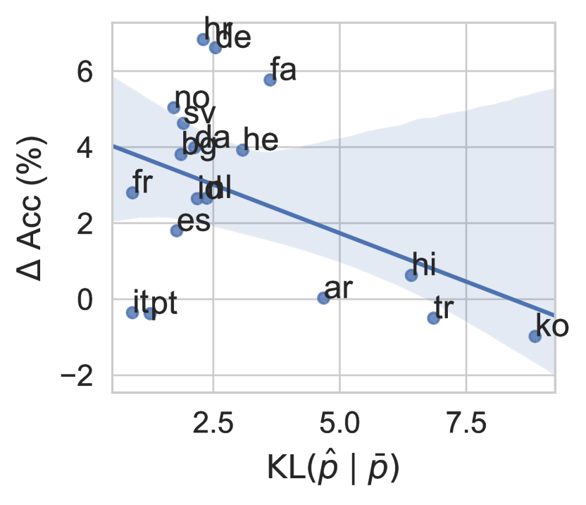
(a) Dependency parsing

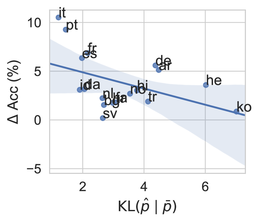
(b) POS tagging

Figure 4: Relationship between $\mathrm{KL}(\hat{p}\mid\bar{p})$ and the accuracy difference of our method and MV, where $\hat{p}$ and $\bar{p}$ denote the empirical true distribution and the opinion pool distribution respectively. Shaded area is $95\text{\,}\mathrm{\char 37\relax}$ confidence interval computed via bootstrapping.

We explore whether there is a relationship between (a) how distant the opinion pool is to the true distribution over substructures and (b) the performance improvement of our method against majority voting. Intuitively, the closer the opinion pool is to the true distribution, the higher its absolute performance would be. However, it is unclear whether this translates into an advantage over majority voting. This is important because if such relationship exists, then it may be worthwhile spending some effort on optimising the opinion pool. To this end, we measure the distance between the true distribution and the opinion pool by computing the Kullback-Leibler divergence (KL)

$$\mathrm{KL}(\hat{p}\mid\bar{p})=\frac{1}{n(\mathcal{D})}\sum_{\boldsymbol{x}\in\mathcal{D}}\sum_{j=1}^{|\boldsymbol{x}|}\mathrm{KL}(\hat{p}_{j}\mid\bar{p}_{j})$$ (12)

where

$$\mathrm{KL}(\hat{p}_{j}\mid\bar{p}_{j})=-\sum_{c\in C(\boldsymbol{x},j)}\hat{p}_{j}(c\mid\boldsymbol{x})\log\left[\frac{\bar{p}_{j}(c\mid\boldsymbol{x})}{\hat{p}_{j}(c\mid\boldsymbol{x})}\right],$$ (13)

$n(\mathcal{D})$ is the total number of tokens of all input sentences in $\mathcal{D}$, $\hat{p}_{j}$ is the (empirical) true distribution of substructures in $C(\boldsymbol{x},j)$, and $\bar{p}_{j}$ is the logarithmic opinion pool distribution defined in Eq. 6. Note that $\hat{p}_{j}$ is a one-hot distribution so $\mathrm{KL}(\hat{p}_{j}\mid\bar{p}_{j})$ reduces to the negative log likelihood of the labelled data under the opinion pool. We compute the KL divergence on the training set of both parsing and tagging and display the regression plots in Fig. 4. We see a medium correlation between opinion pool distance and performance gain against majority voting, with $r=-0.45$ for both parsing and tagging ($p$-value is $0.06$ for both). However, there is substantial variance, especially in the right half figure of parsing, caused by the lack of languages in that region of the plot. Nonetheless, the plots suggest that there is indeed a positive relationship between how close the opinion pool is to the true distribution and the performance gain of our method compared with majority voting.

There are ways to obtain an opinion pool that is closer to the true distribution. One way is to leverage a small amount of labelled data in the target language to estimate the weight factors $\alpha_{k}$, which can be done by optimising Eq. 12. This option is suitable if such labelled data is available or can be obtained cheaply. There is some evidence that 50 samples are enough to estimate similar weight factors in a linear opinion pool (Hu et al. 2021), which may also apply to our setup. If we have the freedom to choose the source languages, another method is to select them carefully so they are both reasonably close to the target language and also diverse. This is because Eq. 12 can be expressed as the difference between two terms, respectively corresponding to how distant the source models’ output distributions are to the target’s true distribution (error) and how distant they are to each other (diversity) (Heskes 1998). Having the source languages reasonably close to the target language and also diverse means reducing the first and increasing the second term respectively, moving the opinion pool closer to the true distribution. That said, when the source languages are close to the target language, the source models may already be good for direct transfer so our method may not give meaningful improvement over majority voting.

Learning the Opinion Pool Weight Factors

	Parsing	Tagging
MV	$56.25$	$65.44$
Uniform $\alpha_{k}$	$58.97$	$69.30$
Learned $\alpha_{k}$	$59.35$	$69.96$

Table 3: Parsing and tagging performance of MV and our method with uniform and learned weight factors $\alpha_{k}$ for the logarithmic opinion pool, averaged over 18 languages.

Motivated by the previous findings, we deviate from our unsupervised setup by learning the weight factors $\alpha_{k}$ using a tiny amount of labelled target data. Concretely, we randomly sample 50 sentences from the training set of each target language and learn $\alpha_{k}$ that minimises Eq. 12 for all source model $k$. We then use the learned weights to obtain the opinion pool as defined in Eq. 6 (see Supplementary Material for further details). Table 3 shows the results on parsing and tagging, averaged over the target languages. We observe that by using the learned weight factors, our method slightly improves over the version using uniform weights, suggesting that our method can readily leverage labelled target data if it is available. On the other hand, the fact that the improvement is only modest also reaffirms that uniform weighting is a strong baseline.

Related Work

A straightforward method of multi-source transfer is training a model on the concatenation of datasets from the source languages. This approach was used by McDonald, Petrov, and Hall (2011) for dependency parsing. They find that this method yields a strong performance gain compared with single-source transfer. More recent work by Guo et al. (2016) proposed to learn multilingual representations from the concatenation of source language data and use them to train a neural dependency parser. Another method is language adversarial training, used by Chen et al. (2019) for various NLP tasks including named-entity recognition, which is another structured prediction problem. Despite their success, multi-source unsupervised cross-lingual transfer methods typically assume access to the source language data, which is not always feasible.

There is recent work suitable in this source-free setup. Rahimi, Li, and Cohn (2019) proposed a method based on truth inference to model label confusion in multi-source transfer of named-entity recognisers. However, extending their method to other structured prediction problems such as dependency parsing is not straightfoward. Wu et al. (2020) used teacher-student learning to transfer from a set of source models as “teachers” to a target model as “student” for named-entity recognition. The method resembles knowledge distillation where the student model is trained to predict soft labels from the teachers, in this case given as a mixture of output distributions. They proposed a method to weight the source models assuming access to unlabelled source data is possible. Hu et al. (2021) argued that in many cases, a small amount of labelled data is available in the target language and proposed an attention-based method to weight the source models leveraging such labelled data for structured prediction. Their best method weights the source models at the substructure level, which can be costly to run.

Our work builds upon the work of Kurniawan et al. (2021) who proposed a method based on self-training for unsupervised cross-lingual dependency parsing. Their multi-source method builds a chart for every unlabelled sample in the target language by combining high probability trees from the source parsers. In this work, we generalise their method to structured prediction problems and propose a modification to improve the quality of the generated charts.

Conclusions

In this paper, we (1) generalise previous methods for cross-lingual unsupervised transfer without source data to structured prediction problems and (2) propose a new aggregation technique which can better handle mixed-quality input distributions. Experiments across two structured prediction tasks and 18 languages show that, unlike previous work, our method generally outperforms a strong multi-source transfer baseline. Our analyses suggest that our method produces distant supervision of better quality than that of the previous methods. Our work potentially generalises beyond language transfer to (a) structured prediction tasks beyond NLP and (b) transfer across other types of domains (e.g., genres), a direction we aim to explore in future work.

Appendix A Supplementary Material

Evaluation Languages

Table 4 lists the languages we use in our evaluation, along with their family, subgroup (if the language is Indo-European), and selected treebanks in Universal Dependencies v2.2. This selection follows Kurniawan et al. (2021) to enable a fair comparison.

Language	Code	Family	UD Treebanks
Distant
Persian	fa	IE.Iranian	Seraji
Arabic	ar	Afro-Asiatic	PADT
Indonesian	id	Austronesian	GSD
Korean	ko	Koreanic	GSD, Kaist
Turkish	tr	Turkic	IMST
Hindi	hi	IE.Indic	HDTB
Croatian	hr	IE.Slavic	SET
Hebrew	he	Afro-Asiatic	HTB
Nearby
Bulgarian	bg	IE.Slavic	BTB
Italian	it	IE.Romance	ISDT
Portuguese	pt	IE.Romance	Bosque, GSD
French	fr	IE.Romance	GSD
Spanish	es	IE.Romance	GSD, AnCora
Norwegian	no	IE.Germanic	Bokmaal, Nynorsk
Danish	da	IE.Germanic	DDT
Swedish	sv	IE.Germanic	Talbanken
Dutch	nl	IE.Germanic	Alpino, LassySmall
German	de	IE.Germanic	GSD

Table 4: List of languages in our evaluation, grouped into distant and nearby languages based on their distance to English (He et al. 2019). IE stands for Indo-European.

Source Models Performance

Table 5 reports the performance of our source parsers and taggers. We also report the performance numbers of previous work, copied from their respective papers, to serve as reference.

	en	ar	es	fr	de
Parsing	$86.9$	$76.9$	$90.0$	$89.1$	$82.1$
Tagging	$94.5$	$95.4$	$96.5$	$96.5$	$92.1$
Previous work (reference only)
LSTM parser	$88.3$	$81.8$	$90.8$	$89.1$	$83.7$
Stanza tagger*	$95.4$	$94.9$	$96.7$	$97.3$	$94.1$

Table 5: Parsing and tagging accuracy of the source models. We copy numbers of the LSTM parser (Ahmad et al. 2019) and Stanza tagger (Qi et al. 2018) from their respective papers to serve as reference only. * indicates that the numbers are not directly comparable to ours because of the difference in the evaluation setup.

Additional Experiment Details

We implement our method using Python v3.7, PyTorch v1.4 (Paszke et al. 2019), and PyTorch-Struct (Rush 2020). We run our experiments with Sacred v0.8.2 (Greff et al. 2017), which also sets the random seeds. Experiments are run on NVIDIA GeForce GTX TITAN X with CUDA 10.1 and GPU memory of 11 MiB. CPU model is Intel(R) Xeon(R) CPU E5-2687W v3 @ 3.10GHz with Ubuntu 16.04 as the operating system.

Hyperparameters

Task	Method	Hyperparameter Dist.	Best Value
Parsing	PPTX	$\log\eta\sim U(-6,-3)$	$\eta=8.5\times 10^{-5}$
		$\log\lambda\sim U(-4,1)$	$\lambda=2.8\times 10^{-5}$
	Ours	$\log\eta\sim U(-6.5,-3.5)$	$\eta=9.4\times 10^{-5}$
		$\log\lambda\sim U(-4,1)$	$\lambda=1.6\times 10^{-4}$
Tagging	PPTX	$\log\eta\sim U(-6,-4)$	$\eta=5.9\times 10^{-5}$
		$\log\lambda\sim U(-4,1)$	$\lambda=0.1$
	Ours	$\log\eta\sim U(-6.5,-3.5)$	$\eta=2.6\times 10^{-4}$
		$\log\lambda\sim U(-4,1)$	$\lambda=4.7\times 10^{-3}$

Table 6: Distributions of hyperparameters we use for tuning on Arabic with random search and the best values found. All logarithms are of base 10.

Hyperparameter	Value
Word embedding size	300
Word dropout	0.2
$d_{\text{key}},d_{\text{value}}$	64
$d_{\text{ff}}$	512
$n_{\text{head}}$	8
$n_{\text{layer}}$	6
Batch size	80
Parsing-only
POS tag embedding size	50
Output embedding dropout	0.2
$d_{\text{arc}}$	512
$d_{\text{deptype}}$	128

Table 7: List of hyperparameter values used in our parsers and taggers. $d_{\text{key}},d_{\text{value}}$: size of key and value vector in the Transformer encoder. $d_{\text{ff}}$: size of feedforward network hidden layer in the Transformer encoder. $n_{\text{head}}$: number of heads in the Transformer encoder. $n_{\text{layer}}$: number of layers in the Transformer encoder. $d_{\text{arc}},d_{\text{deptype}}$: size of feedforward network output layer corresponding to arcs and dependency types in the biaffine output layer of parsers.

We tune learning rate $\eta$ and $\lambda$ using random search. Table 6 shows the distributions of each hyperparameter we use, and the best values we find. We sample 20 values from the distribution and pick the values that yield the best accuracy on the Arabic development set. We follow Kurniawan et al. (2021) for other hyperparameters, whose values are reported in Table 7.

Learning the Opinion Pool Weight Factors

We learn the factors $\alpha_{k}$ weighting the contribution of source model $k$ in the logarithmic opinion pool by minimising Eq. 12 with respect to $\alpha_{k}$. The minimisation is done on 50 randomly sampled sentences from the target language’s training set using gradient descent. We set the initial learning rate to $0.1$ and reduce it at every epoch by a factor of $0.9$. We initialise the weight factors uniformly at the start and run the training until convergence. After the weight factors are learned, we use and fix them for all subsequent experiments. We proceed with hyperparameter tuning on Arabic using the same procedure as the version with uniform weights. For both tasks, we tune $\eta$ and $\lambda$ with random search (20 runs), drawing from $\log_{10}\eta\sim U(-6,-3)$ and $\log_{10}\lambda\sim U(-4,1)$ respectively. For parsing, the best values are $\eta=9.1\times 10^{-5}$ and $\lambda=5.1\times 10^{-4}$. For tagging, they are $\eta=4.7\times 10^{-4}$ and $\lambda=0.062$. These values are then used for the other languages. Lastly, we report the average accuracy over the languages in Table 3.

Full Experiment Results

We report in Table 8 the full results of MV, PPTX, and our method (with both uniform and learned weight factors $\alpha_{k}$) on both dependency parsing and POS tagging, averaged over 5 runs.

Language	Parsing				Tagging
	MV	PPTX	Ours	Ours, learned $\alpha_{k}$	MV	PPTX	Ours	Ours, learned $\alpha_{k}$
Distant
fa	$43.7$	$42.5\pm 1.1$	$49.4\pm 0.5$	$48.9\pm 0.3$	$69.2$	$67.5\pm 0.2$	$71.2\pm 0.6$	$72.3\pm 0.5$
ar	$37.6$	$36.4\pm 0.6$	$38.9\pm 0.5$	$38.6\pm 0.5$	$58.5$	$59.0\pm 0.4$	$62.5\pm 1.1$	$63.0\pm 1.7$
id	$56.8$	$54.8\pm 0.8$	$59.0\pm 0.3$	$59.1\pm 0.1$	$77.5$	$79.6\pm 0.4$	$81.0\pm 0.2$	$80.6\pm 0.8$
ko	$13.7$	$13.6\pm 0.4$	$12.8\pm 0.3$	$13.6\pm 0.2$	$44.1$	$44.0\pm 0.3$	$44.2\pm 1.1$	$43.4\pm 1.7$
tr	$20.8$	$19.9\pm 0.2$	$20.2\pm 0.4$	$21.2\pm 0.2$	$62.8$	$62.8\pm 0.3$	$64.2\pm 0.3$	$64.3\pm 0.2$
hi	$21.9$	$23.9\pm 0.5$	$22.7\pm 0.2$	$27.2\pm 0.2$	$59.9$	$65.6\pm 0.2$	$63.2\pm 0.6$	$65.5\pm 0.9$
hr	$57.1$	$60.7\pm 0.3$	$62.9\pm 0.4$	$62.8\pm 0.3$	$67.2$	$58.6\pm 0.1$	$69.4\pm 0.3$	$69.7\pm 0.3$
he	$56.1$	$58.1\pm 0.5$	$60.6\pm 0.2$	$60.0\pm 0.2$	$56.3$	$57.6\pm 0.1$	$59.9\pm 0.2$	$58.8\pm 0.5$
Nearby
bg	$69.3$	$71.9\pm 0.2$	$72.7\pm 0.4$	$72.5\pm 0.4$	$75.0$	$75.9\pm 0.2$	$76.7\pm 0.2$	$76.1\pm 0.2$
it	$81.5$	$80.1\pm 0.2$	$81.7\pm 0.2$	$81.5\pm 0.1$	$74.7$	$62.8\pm 0.7$	$84.8\pm 0.3$	$85.5\pm 0.7$
pt	$78.6$	$76.2\pm 0.4$	$78.1\pm 0.3$	$78.4\pm 0.3$	$72.0$	$63.5\pm 0.9$	$81.7\pm 0.4$	$83.2\pm 1.0$
fr	$80.0$	$81.3\pm 0.2$	$82.7\pm 0.2$	$82.8\pm 0.1$	$65.7$	$54.9\pm 0.5$	$71.7\pm 0.7$	$76.3\pm 0.7$
es	$71.8$	$72.0\pm 0.6$	$73.5\pm 0.3$	$73.7\pm 0.2$	$67.8$	$58.1\pm 0.2$	$73.9\pm 0.7$	$75.7\pm 2.1$
no	$68.4$	$74.1\pm 0.2$	$74.2\pm 0.1$	$74.4\pm 0.2$	$62.2$	$61.4\pm 0.2$	$64.7\pm 0.5$	$64.6\pm 1.1$
da	$67.5$	$70.4\pm 0.4$	$71.0\pm 0.1$	$70.9\pm 0.3$	$72.9$	$72.0\pm 0.1$	$76.0\pm 0.3$	$76.2\pm 0.7$
sv	$66.7$	$71.8\pm 0.2$	$72.1\pm 0.1$	$72.4\pm 0.5$	$68.4$	$68.5\pm 0.1$	$69.0\pm 0.4$	$70.7\pm 0.6$
nl	$64.8$	$66.9\pm 0.2$	$67.4\pm 0.4$	$68.8\pm 0.4$	$72.9$	$70.3\pm 0.3$	$74.3\pm 0.4$	$75.3\pm 0.7$
de	$57.2$	$64.0\pm 0.9$	$64.0\pm 0.5$	$63.9\pm 0.5$	$52.8$	$59.3\pm 0.3$	$58.9\pm 0.5$	$58.0\pm 0.4$

(a) Development set

Language	Parsing				Tagging
	MV	PPTX	Ours	Ours, learned $\alpha_{k}$	MV	PPTX	Ours	Ours, learned $\alpha_{k}$
Distant
fa	$43.7$	$42.5\pm 1.0$	$49.4\pm 0.4$	$48.8\pm 0.3$	$69.4$	$67.4\pm 0.3$	$71.1\pm 0.7$	$72.5\pm 0.7$
ar	$37.3$	$35.5\pm 0.5$	$37.3\pm 0.5$	$37.2\pm 0.6$	$57.8$	$59.0\pm 0.5$	$63.0\pm 1.4$	$63.3\pm 1.6$
id	$59.0$	$57.4\pm 0.6$	$61.6\pm 0.2$	$61.4\pm 0.2$	$77.9$	$79.9\pm 0.4$	$81.0\pm 0.2$	$80.8\pm 0.8$
ko	$14.7$	$14.8\pm 0.5$	$13.8\pm 0.4$	$14.7\pm 0.1$	$45.0$	$45.7\pm 0.2$	$45.9\pm 1.1$	$44.9\pm 1.5$
tr	$20.1$	$19.3\pm 0.2$	$19.7\pm 0.3$	$20.8\pm 0.2$	$62.8$	$63.0\pm 0.2$	$64.7\pm 0.5$	$64.9\pm 0.1$
hi	$21.1$	$23.0\pm 0.5$	$21.7\pm 0.2$	$26.4\pm 0.3$	$59.7$	$65.1\pm 0.2$	$62.8\pm 0.5$	$65.1\pm 1.0$
hr	$57.4$	$62.2\pm 0.2$	$64.3\pm 0.4$	$64.2\pm 0.3$	$66.7$	$58.4\pm 0.1$	$68.5\pm 0.2$	$69.0\pm 0.4$
he	$56.2$	$57.5\pm 0.7$	$60.1\pm 0.2$	$59.7\pm 0.3$	$55.5$	$57.2\pm 0.1$	$59.1\pm 0.4$	$58.0\pm 0.4$
Nearby
bg	$69.3$	$72.4\pm 0.2$	$73.1\pm 0.3$	$72.9\pm 0.3$	$75.6$	$76.2\pm 0.1$	$77.1\pm 0.3$	$76.6\pm 0.2$
it	$81.7$	$80.2\pm 0.1$	$81.4\pm 0.2$	$81.4\pm 0.3$	$74.5$	$62.1\pm 0.8$	$85.0\pm 0.4$	$86.0\pm 0.8$
pt	$76.6$	$74.5\pm 0.4$	$76.3\pm 0.3$	$76.5\pm 0.3$	$72.5$	$63.4\pm 0.8$	$81.8\pm 0.5$	$83.1\pm 0.9$
fr	$76.5$	$78.2\pm 0.3$	$79.3\pm 0.1$	$79.1\pm 0.1$	$65.4$	$56.0\pm 0.4$	$72.2\pm 0.6$	$75.7\pm 0.5$
es	$71.3$	$71.5\pm 0.6$	$73.1\pm 0.4$	$73.2\pm 0.3$	$67.1$	$57.8\pm 0.2$	$73.5\pm 0.6$	$75.1\pm 2.0$
no	$69.1$	$74.1\pm 0.2$	$74.2\pm 0.2$	$74.5\pm 0.2$	$63.2$	$62.3\pm 0.3$	$65.9\pm 0.6$	$65.7\pm 1.1$
da	$67.3$	$70.7\pm 0.3$	$71.3\pm 0.1$	$71.2\pm 0.4$	$73.9$	$72.8\pm 0.1$	$77.1\pm 0.4$	$77.3\pm 0.6$
sv	$70.1$	$74.5\pm 0.3$	$74.7\pm 0.2$	$75.0\pm 0.3$	$69.8$	$69.6\pm 0.1$	$70.0\pm 0.3$	$72.0\pm 0.5$
nl	$65.8$	$67.8\pm 0.4$	$68.5\pm 0.3$	$69.6\pm 0.4$	$70.8$	$68.7\pm 0.3$	$73.0\pm 0.3$	$74.5\pm 1.0$
de	$55.3$	$61.6\pm 0.8$	$61.9\pm 0.6$	$61.7\pm 0.5$	$50.2$	$56.4\pm 0.3$	$55.8\pm 0.6$	$54.9\pm 0.4$

(b) Test set

Table 8: Full performance results. Numbers are averages ($\pm$ std) over 5 runs with different random seeds. For parsing, the numbers correspond to labelled attachment score (LAS) whereas for tagging, they correspond to accuracy. Both metrics are better if higher.

References

- Ahmad et al. (2019) Ahmad, W.; Zhang, Z.; Ma, X.; Hovy, E.; Chang, K.-W.; and Peng, N. 2019. On Difficulties of Cross-Lingual Transfer with Order Differences: A Case Study on Dependency Parsing. In Proceedings of the 2019 Conference of the North American Chapter of the Association for Computational Linguistics: Human Language Technologies, Volume 1 (Long and Short Papers), 2440–2452.
- Böhmová et al. (2003) Böhmová, A.; Hajič, J.; Hajičová, E.; and Hladká, B. 2003. The Prague Dependency Treebank. In Abeillé, A., ed., Treebanks: Building and Using Parsed Corpora, 103–127. ISBN 978-94-010-0201-1.
- Bojanowski et al. (2017) Bojanowski, P.; Grave, E.; Joulin, A.; and Mikolov, T. 2017. Enriching Word Vectors with Subword Information. Transactions of the Association for Computational Linguistics, 5: 135–146.
- Brants, Skut, and Uszkoreit (2003) Brants, T.; Skut, W.; and Uszkoreit, H. 2003. Syntactic Annotation of A German Newspaper Corpus. In Abeillé, A., ed., Treebanks: Building and Using Parsed Corpora, 73–87. ISBN 978-94-010-0201-1.
- Chen et al. (2019) Chen, X.; Awadallah, A. H.; Hassan, H.; Wang, W.; and Cardie, C. 2019. Multi-Source Cross-Lingual Model Transfer: Learning What to Share. In Proceedings of the 57th Annual Meeting of the Association for Computational Linguistics, 3098–3112.
- Chu and Liu (1965) Chu, Y.-J.; and Liu, T.-H. 1965. On the Shortest Arborescence of a Directed Graph. Scientia Sinica, 14: 1396–1400.
- Dozat and Manning (2017) Dozat, T.; and Manning, C. D. 2017. Deep Biaffine Attention for Neural Dependency Parsing. In International Conference on Learning Representations, 8.
- Duong et al. (2015) Duong, L.; Cohn, T.; Bird, S.; and Cook, P. 2015. Cross-Lingual Transfer for Unsupervised Dependency Parsing without Parallel Data. In Proceedings of the Nineteenth Conference on Computational Natural Language Learning, 113–122.
- Edmonds (1967) Edmonds, J. 1967. Optimum Branchings. Journal of Research of the national Bureau of Standards B, 71(4): 233–240.
- Greff et al. (2017) Greff, K.; Klein, A.; Chovanec, M.; Hutter, F.; and Jürgen Schmidhuber. 2017. The Sacred Infrastructure for Computational Research. In Huff, K.; Lippa, D.; Niederhut, D.; and M Pacer, eds., Proceedings of the 16th Python in Science Conference, 49–56.
- Guo et al. (2016) Guo, J.; Che, W.; Yarowsky, D.; Wang, H.; and Liu, T. 2016. A Representation Learning Framework for Multi-Source Transfer Parsing. In Thirtieth AAAI Conference on Artificial Intelligence.
- He et al. (2019) He, J.; Zhang, Z.; Berg-Kirkpatrick, T.; and Neubig, G. 2019. Cross-Lingual Syntactic Transfer through Unsupervised Adaptation of Invertible Projections. In Proceedings of the 57th Annual Meeting of the Association for Computational Linguistics, 3211–3223.
- Heskes (1998) Heskes, T. 1998. Selecting Weighting Factors in Logarithmic Opinion Pools. In Jordan, M.; Kearns, M.; and Solla, S., eds., Advances in Neural Information Processing Systems, volume 10.
- Hu et al. (2021) Hu, Z.; Jiang, Y.; Bach, N.; Wang, T.; Huang, Z.; Huang, F.; and Tu, K. 2021. Multi-View Cross-Lingual Structured Prediction with Minimum Supervision. In Proceedings of the 59th Annual Meeting of the Association for Computational Linguistics and the 11th International Joint Conference on Natural Language Processing (Volume 1: Long Papers), 2661–2674.
- Joshi et al. (2020) Joshi, P.; Santy, S.; Budhiraja, A.; Bali, K.; and Choudhury, M. 2020. The State and Fate of Linguistic Diversity and Inclusion in the NLP World. In Proceedings of the 58th Annual Meeting of the Association for Computational Linguistics.
- Kurniawan et al. (2021) Kurniawan, K.; Frermann, L.; Schulz, P.; and Cohn, T. 2021. PPT: Parsimonious Parser Transfer for Unsupervised Cross-Lingual Adaptation. In Proceedings of the 16th Conference of the European Chapter of the Association for Computational Linguistics: Main Volume, 2907–2918.
- McClosky, Charniak, and Johnson (2006) McClosky, D.; Charniak, E.; and Johnson, M. 2006. Effective Self-Training for Parsing. In Proceedings of the Human Language Technology Conference of the NAACL, Main Conference, 152–159.
- McDonald et al. (2005) McDonald, R.; Pereira, F.; Ribarov, K.; and Hajič, J. 2005. Non-Projective Dependency Parsing Using Spanning Tree Algorithms. In Proceedings of Human Language Technology Conference and Conference on Empirical Methods in Natural Language Processing, 523–530.
- McDonald, Petrov, and Hall (2011) McDonald, R.; Petrov, S.; and Hall, K. 2011. Multi-Source Transfer of Delexicalized Dependency Parsers. In Proceedings of the 2011 Conference on Empirical Methods in Natural Language Processing, 62–72.
- Nivre et al. (2018) Nivre, J.; Abrams, M.; Agić, Ž.; and et al. 2018. Universal Dependencies 2.2. LINDAT/CLARIAH-CZ digital library at the Institute of Formal and Applied Linguistics (ÚFAL), Faculty of Mathematics and Physics, Charles University.
- Pan and Yang (2010) Pan, S. J.; and Yang, Q. 2010. A Survey on Transfer Learning. IEEE Transactions on Knowledge and Data Engineering, 22(10): 1345–1359.
- Paszke et al. (2019) Paszke, A.; Gross, S.; Massa, F.; Lerer, A.; Bradbury, J.; Chanan, G.; Killeen, T.; Lin, Z.; Gimelshein, N.; Antiga, L.; Desmaison, A.; Kopf, A.; Yang, E.; DeVito, Z.; Raison, M.; Tejani, A.; Chilamkurthy, S.; Steiner, B.; Fang, L.; Bai, J.; and Chintala, S. 2019. PyTorch: An Imperative Style, High-Performance Deep Learning Library. In Wallach, H.; Larochelle, H.; Beygelzimer, A.; dAlché-Buc, F.; Fox, E.; and Garnett, R., eds., Advances in Neural Information Processing Systems 32, 8024–8035.
- Qi et al. (2018) Qi, P.; Dozat, T.; Zhang, Y.; and Manning, C. D. 2018. Universal Dependency Parsing from Scratch. In Proceedings of the CoNLL 2018 Shared Task: Multilingual Parsing from Raw Text to Universal Dependencies, 160–170.
- Rahimi, Li, and Cohn (2019) Rahimi, A.; Li, Y.; and Cohn, T. 2019. Massively Multilingual Transfer for NER. In Proceedings of the 57th Annual Meeting of the Association for Computational Linguistics, 151–164.
- Rush (2020) Rush, A. 2020. Torch-Struct: Deep Structured Prediction Library. In Proceedings of the 58th Annual Meeting of the Association for Computational Linguistics: System Demonstrations, 335–342.
- Smith et al. (2017) Smith, S. L.; Turban, D. H. P.; Hamblin, S.; and Hammerla, N. Y. 2017. Offline Bilingual Word Vectors, Orthogonal Transformations and the Inverted Softmax. In International Conference on Learning Representations.
- Wu et al. (2020) Wu, Q.; Lin, Z.; Karlsson, B.; LOU, J.-G.; and Huang, B. 2020. Single-/Multi-Source Cross-Lingual NER via Teacher-Student Learning on Unlabeled Data in Target Language. In Proceedings of the 58th Annual Meeting of the Association for Computational Linguistics, 6505–6514.