Monte Carlo simulation of COVID-19 pandemic using statistical physics-inspired probabilities

Abstract

We present a Monte Carlo simulation model of an epidemic spread inspired on physics variables such as temperature, cross section and interaction range, which considers the Plank distribution of photons in the black body radiation to describe the mobility of individuals. The model consists of a lattice of cells that can be in four different states: susceptible, infected, recovered or death. An infected cell can transmit the disease to any other susceptible cell within some random range $R$. The transmission mechanism follows the physics laws for the interaction between a particle and a target. Each infected particle affects the interaction region a number $n$ of times, according to its energy. The number of interactions is proportional to the interaction cross section $\sigma$ and to the target surface density $\rho$. The discrete energy follows a Planck distribution law, which depends on the temperature $T$ of the system. For any interaction, infection, recovery and death probabilities are applied. We investigate the results of viral transmission for different sets of parameters and compare them with available COVID-19 data. The parameters of the model can be made time dependent in order to consider, for instance, the effects of lockdown in the middle of the pandemic.

url]webpage: http://www.ugr.es/$\sim$amaro

url]https://nuclear.uwc.ac.za

1 Introduction

The COVID-19 pandemic, that has so far caused almost five million deaths worldwide [1, 2], has recently induced numerous studies on the mathematical modelling of temporal distributions of infected cases and fatalities [3, 4, 5, 6, 7]. Various statistical models for pandemic spread and their predictive power have been benchmarked against data [8, 9].

The SIR (susceptible-infected-recovered) model – developed by Kermack and McKendric [10] – and derived models are the most widely used to study viral spreading of contagious epidemics or mass immunization planning [11, 12, 13] since they provide mean values of the cumulative incidence as a function of time in a deterministic way. SIR models belong to the compartmental type, where the equations only involve the time variable, and the incidence functions refer to the total number of individuals in each compartment or subset of the total number of individuals in the system.

Generalization to more realistic models of the infection transmission process requires solving spatio-temporal equations [14] in a two-dimensional space representing the surface of a region under epidemics. Such individual-level models were first studied by Kendall [15] and Bartlett [16, 17], who also considered both deterministic and stochastic kind of descriptions.

In this paper we present a study of space-time propagation of a viral infection using a new stochastic model inspired by concepts of statistical physics and nuclear physics. This model is compared to a simple compartment model developed in ref. [9] (the D model), where we studied the accumulated fatalities for a series of countries during the first COVID-19 wave.

The purpose of this work is to present the Monte Carlo Planck (MCP) model in order to study the stochastic behavior of the spatio-temporal propagation, to test the predictive power of these kind of models with respect to COVID-19 available data as well as to assess the validity of the D model.

Further Monte Carlo-type studies have been developed to simulate the pandemic transmission [19, 20, 18], but use other approaches such as, for instance, a 2D-random walk Monte Carlo simulation based on proximity infection spread. In the present MCP model we take a physical point of view, where the infection is a result of an interaction, and it follows to some extent statistical laws similar to the interaction in a system of many particles. Thus we model the infection as a likely result of a physical interaction. We apply concepts taken from statistical and nuclear physics such as interaction range, energy, temperature, and interaction cross section. These concepts, adapted to the present case of interest, are useful to describe probability distributions and interaction coefficients in physical systems, which are here characterized by epidemiological probabilities of infection, recovery and death.

In Section 2 we present the MCP model. In Section 3 we present results of the simulation applied to COVID-19 fatalities data for several countries. Finally in Sect. 4 we draw our conclusions.

2 The Monte Carlo Planck model

We consider the system of a two-dimensional lattice or grid, where each unit cell has two coordinates $k=(k_{1},k_{2})$, with $k_{i}=1,2,\ldots,L$, where $L$ is the total size of the system, with surface $L^{2}$. Each cell $k$ is occupied by an individual, who can be in any of four states or classes: susceptible, infected, recovered or dead. This state is specified by four fields or matrices $s(k)$, $i(k)$, $r(k)$, and $d(k)$ that can take the values 1 or 0 (state quantum numbers) , depending whether the individual in cell $k$ belongs or not to the corresponding class. The model can be easily extended to include other classes or intermediate states.

In the initial state, for $t=0$, all the individuals are susceptible. Then

$$s(k)=1,\kern 28.45274pti(k)=r(k)=d(k)=0$$ (1)

for all $k$ except for one initially infected cell $k_{0}$, where

$$s(k_{0})=0,\kern 28.45274pti(k_{0})=1.$$ (2)

We choose the initial infected cell at the center of the grid, but in the model it can be chosen randomly or even to be several infected cells.

In the simulation we compute the state of the system in time intervals of $\Delta t=1$ day. At the end of the day, $t=1,2,3,\ldots$, we compute and store in the matrices $s$, $i$, $r$, $d$ the current state of the system. We also store the total number of susceptible $S(t)$, infected, $I(t)$, recovered, $R(t)$ and dead, $D(t)$ and the daily increments, $\Delta S(t)$, $\Delta I(t)$, $\Delta R(t)$, $\Delta D(t)$, and repeat the calculation for the next day.

In the simulation for day $t$ we apply the following algorithm to each cell $k$.

1. If it is not infected, $i(k)=0$, do nothing.

2. It it is infected, $i(k)=1$, then we assume that it can infect only people in other cells within a finite region of size $R$. The value of the range $R$ takes into account the zone of influence of individuals in one day. To simplify the algorithm in Cartesian coordinates we assume that the region is a square of side $2R$, centered at the cell $k$, but it could be also circular or other shape.

   Now the Monte Carlo starts by computing the value of $R$ randomly with some probability distribution. We assume an exponential law

   $$P(R)=\frac{{\rm e}^{-R/R_{0}}}{R_{0}},$$ (3)

   which indicates that is less probable to move far away from the average interaction range $R_{0}$ of the individuals. This is one of the parameters of the model.

3. Once $R$ is chosen for an infected particle, it can interact randomly with any of the $N_{R}$ individuals within the region with area $S_{R}$. As in particle physics, we characterize the interaction between individuals by a cross section $\sigma$. The number of possible interactions is then given by the probability formula when $n$ particles are shot over a target

   $$N_{\rm int}=nN_{R}\frac{\sigma}{S_{R}}=n\rho\sigma,$$ (4)

   where $\rho=1$ is the surface density and the number of shots $n$ is related with the mobility of the individual within its zone of influence, indicating if it has a narrow social behaviour and how often it moves around each day. We call this property the energy of the individuals. For instance, Young people have more energy than old people, or people with a job where they interact often with other people. We compute the value of the energy $n$ randomly with an energy distribution. In analogy to the Planck law for photons from statistical physics, we write the energy distribution in a simplified form as

   $$P(n)=\frac{{\rm e}^{-n/T}}{{\rm e}^{1/T}-1},$$ (5)

   where the parameter $T$ is the temperature of the system that determines the average energy or number of shots.

   In this work we choose unit cells and therefore assume $\rho=1$ in arbitrary units, but the model can be modified to include specific densities and sample population sizes with known number of individuals. In the model the information on the density is included in the range $R_{0}$. To increase the density is equivalent to increase the range and the temperature. The result of this work are given for unit density and the values of $R_{0}$ and $T$ should be appropriately re-scaled to apply the results to different densities.

4. Once we know the range $R$ and the number of interactions $N_{\rm int}$ of an infected cell, we choose randomly $N_{\rm int}$ cells, with coordinates $k^{\prime}$, within the interaction region. If cell $k^{\prime}$ is susceptible, $s(k^{\prime})=1$, it can be infected with probability $0\leq p_{i}\leq 1$. We then decide randomly it it is infected or not according to that probability. In case that it becomes infected, we change the vaue of the corresponding matrix elements $s(k^{\prime})=0$ and $i(k^{\prime})=1$. We also store the time it becomes infected in the infection time matrix $\Theta(k)=t$. This matrix is important for the nex step in deciding when the particle becomes recovered or dead.

5. After interacting with all the $N_{\rm int}$ individuals within the range $R$, along the day, finally we decide if cell $k$ becomes recovered or dead at night. We assume that the removal probability depends on time with a function

   $$P_{\rm rem}(t)=\frac{1}{1+{\rm e}^{(t_{r}-t)/b}},$$ (6)

   where $t_{r}$ is the time such that $P(t_{r})=1/2$ and $t_{r}\gg b$, so that the removal probability is very small for low times, and later it increases with time at a rate driven by the parameter $b$. For $t\rightarrow\infty$, the removal probability is one. All the individuals recover or die.

   Therefore we randomly decide if $k$ is removed at the end of the day with a probability $P_{\rm rem}(t-\Theta(k))$ that depend on the time $t-\Theta(k)$ that particle $k$ has been infected. In case $k$ is removed, we change the state quantum number in the infected matrix, $i(k)=0$.

6. The final step, if particle is removed, we decide if it is dead randomly with probability $P_{\rm d}\leq 1$. Otherwise it is recovered. Finally we store the matrices $r(k)=1$ (0), and $d(k)=0$ (1) accordingly.

7. We repeat the procedure on the next cell.

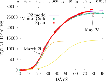
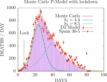
Figure 1: Fit of the P-model to the cumulative deaths and deaths per day by COVID-19 in Spain during the first wave. The red points are the data compiled up to May 25, 2020. The two yellow lines in the left panel are the two D-functions appearing in the D2 model, Eq. (7).

The algorithm so defined depends on the following parameters

• The size of the system $L$, The unit of length in natural units, is the average distance between individuals. This determines the number of cells $L^{2}$.

• The range of interaction $R_{0}$, indicating the maximum distance on average that the infection can propagate in one day. This parameter can be time dependent, and, by changing it, one can simulate for instance lockdown or long travels in holidays.

• The cross section $\sigma$ measures the probability of interaction between two individuals. In the case of classical particles interacting with contact forces the cross sections is just the effective geometrical area of the pair. For long range forces the cross section is larger. In our case it is typically much larger than the geometrical human size, because this parameter takes into account the human behavior. Humans move and are social increasing its cross section, like a long range force.

• The temperature of the system, $T$ determines the average energy of the individuals, which is related to the movility within its range of interaction.

• The infection probability $0\leq p_{i}\leq 1$

• The removal probability parameters $t_{r}$ and $b$ (two parameters).

• The death probability of removed $p_{d}$

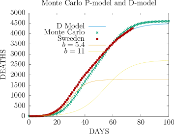
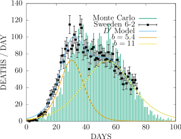
Figure 2: Fit of the P-model to the cumulative deaths and deaths per day by COVID-19 in Sweden during the first wave.

These are in total 8 parameters $L$, $R_{0}$, $\sigma$, $T$, $p_{i}$, $a$, $b$ and $p_{d}$. In addition, each one of these parameters can be easily made time dependent to study the effects of political enforcement, lockdown, social distancing, large events, etc. The model could also be modified easily to include coordinate dependence of the parameters to specify for instance a large event in some region by increasing the temperature or the cross section in that region.

Actually one can argue that increasing temperature, increasing cross section and increasing the infection probability are expected to produce similar effects on the pandemic evolution, and that the pandemic evolution is effectively driven by less parameters, perhaps six or less, unless time or space dependence (or non constant densities) is introduced in them.

In the next section we fit the parameters of this MCP model to describe data from the first wave of the COVID-19 pandemic.

3 Results

Firstly, the MCP model requires fixing the number of individuals, which is equal to the area $N=L^{2}$ of the square lattice (each individual occupies one square). To make the calculation manageable, we chose an initial size of $L=300$, that is $N=90,000$ individuals in the sample, although we latter also consider the effect of making L larger. Obviously, if the number of deaths exceeds this figure, to study a more realistic case, a size comparable to the population of the country in question should be considered. But in this first simulation we prefer to make the model as simple and manageable as possible in order to investigate whether under these simplifications it is still possible to describe the data.

An important detail is that, given the probability of death $p_{D}$, the expected mean number of deaths is fixed from the beginning $D(\infty)\simeq Np_{D}$. If this value is not known experimentally, we first fix it by fitting a SIR-type model to the incomplete data. Specifically, we apply the D- and D2-models of Ref. [9], which consist of sums of logistic functions, to estimate the probability of death before doing the Monte Carlo. The death number as a function of time in the D-model is

$$D(t)=\frac{a}{{\rm e}^{-(t-t_{0})/b}+c},$$ (7)

where the three parameters $a,b,c$ are fitted to data and the initial time $t_{0}$ is arbitrary. In the case of the D2-model we fit the sum of two D-functions with six parameters $a_{1},b_{1},c_{1},a_{2},b_{2},c_{2}$ in total. This provides a method for estimating a prediction for the total number of deaths $D(\infty)=a/c$ ($a_{1}/c_{1}+a_{2}+c_{2}$ in the case of the D2-model). This value $D(\infty)$ is used as input to set the parameters of the Monte Carlo simulation since we know that the D model works well as a starting point for pandemic forecasting [9]. Thus the Monte Carlo will be useful to study the stochastic distribution of daily cases, since the SIR models only provide the mean values without statistical fluctuations.

Table 1: Parameters of the MCP model for Spain, Sweden and South Africa. The value of the range $R_{0}$ during lockdown in Spain and the temperature $T$ during gathering restrictions in Sweeden are in parentheses.

$L$ $R_{0}$ $\rho\sigma$ $T$ $t_{r}$ $b$ $p_{i}$ $p_{d}$ (days) (days) Spain First wave 300 8 (3) 0.1 20 20.7 4.5 0.2 0.3 Sweden First wave 300 10 0.3 20 (15) 24 4 0.2 0.3 South Africa First wave 300 2.9 0.09 20 20 4 0.15 0.2 Second wave 300 3 0.1 20 20 4 0.15 0.5

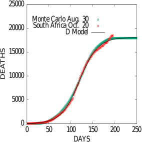
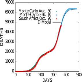
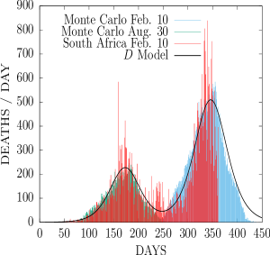
Figure 3: Fit of MCP model to the cumulative deaths by coronavirus in South Africa during the first (left) and second (middle) pandemic waves, together with the overall daily deaths (right). Data from [23] fitted up to Feb. 10 2021.

The simulation was started assuming that in the initial instant $t=0$ there is an infected individual in the central cell of the array and all the others cells are susceptible. The algorithm of the previous sections is then applied by assuming time steps $\Delta t=1$ day. In Figure 1 we show the results of the Monte Carlo simulation of the deaths-per-day, $\Delta(t)$, in Spain. We fitted the data until May 30, 2020, where clearly the first COVID-19 wave had practically ended. We first fitted the D2 model (as the sum of two logistic functions) to the data to better estimate the end of the epidemic, and then we fitted the MCP paremeters to the curve of total accumulated deaths $D(t)$ of the D2-model. It is worth mentioning that fitting the Monte Carlo to the accumulated deaths curve is more reliable than fitting the daily data, $\Delta D(t)$, and gives better results. This is because the cumulative curve data has less fluctuations and less error than the daily data.

The MCP parameters are given in Table 1. The parameters of Table 1 have been tuned to describe the experimental data, including the lockdown. In general The Monte Carlo points have to be shifted in time ($\Delta t=12$ days in the Spain case) to agree with the center of the experimental peak, that has a different time origin. This is so because there is an arbitrariness regarding the start of the pandemic.

For Spain, the MCP simulation includes lockdown effect on day 20, where the value of the range was reduced to $R_{0}=3$ (fitted also to the data). In Spain the lockdown started on day 14M (March 14), corresponding to day 7 in the plot of Fig.1, and the maximum of the daily deaths, $\Delta D(t)$, occurred on 2A (April 2), corresponding to day 26 in the plot. The distance between maximum and lockdown therefore is $t_{\max}-t_{L}=26-7=19$ days. In the the MCP simulation this distance is 15 days.

From the results of Fig. 1 we see that the MCP and the D2 models present the same trend. Both models describe the death data, both total and daily deaths, very similarly. This means that the hypothesis of the MCP model that the spread of infection can be described by physical interactions in a system of many particles is correct, since it agrees with the statistical model of the SIR type and is able to describe the experimental data of the pandemic.

The main difference with the D2 statistical model is that the MCP acquires random statistical fluctuations, which the SIR models do not have, since they only describe mean values. We also see that the fluctuations in the data are much larger than in our model, even considering the statistical errors of the daily data. These values have been taken from the Poisson distribution $\Delta n=\sqrt{n}$. However it must be taken into account that the official death data have systematic errors due to the data collection methods and delays, and that these errors could be quite large. In such cases it may be reasonable to first compute a moving average of the data over three or more days to reduce fluctuations before fitting the models.

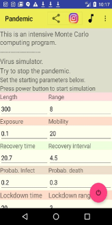
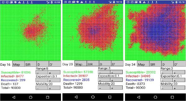
Figure 4: Monte Carlo Plank model simulator for Androids illustrating how the pandemic spreads in a lattice of length $L=300$ – which corresponds to a population of $L^{2}=N=90000$ – as a function of time.

Concerning the values of the parameters, the death probability $p_{D}=0.3$ is fixed by the total fatalities. In Spain the three physical parameters are the following. The initial range $R_{0}=8$, later changed to $R_{0}=3$ after the first week to take into account the lockdown. The temperature or mobility $T=20$, means that in average 20 shots are used to compute the interaction in Eq. (4). The cross section multiplied by the density gives the probability of interaction between cells $\rho\sigma=0.1$. This means about 2 interactions in average. The infection probability is $p_{I}=0.2$. Finally the recovery time is $t_{r}=20.7$ days and the recovery interval $b=4.5$ days These parameters give an idea of how long the infection lasts, until there is recovery or death, which is around three weeks.

In Figure 2 we show a simulation of the case of Sweden. In order to keep the probability of death equal to the Spanish one, we have randomly chosen 85% of the cells with total lockdown, which produces the same effect as reducing the size of the susceptible ones, in order to obtain the number of deaths from the first or $~{}4500$. As a result, the value obtained for the range is larger than in Spain $R_{0}=10$, and also the value of $\rho\sigma=0.3$. In Sweden there was no lockdown and this value does not change in time. But in Sweden there was a gathering restriction that no more than 10 people could meet. This has been simulated in the Monte Carlo by lowering the temperature from $T=20$ to $T=15$ during gathering restrictions. The gathering day here has been taken equal to 40. The recovery time $t_{r}=24$ is about three days larger than in Spain.

In Figure 3 we present results in the case of South Africa. The first and second waves are well differentiated and each of them can be described separately with model D. This is what has been done in the figure, adjusting the data for each wave separately. In the same way, the MCP model has been adjusted here separately for each of the two waves. The first Monte Carlo was adjusted for data through August 30, 2020. The second Monte Carlo was adjusted for data from the second from this date through February 10, 2021. Each Monte Carlo simulation has been adjusted independently with a lattice of $L=300$. That is why the probability of death in the first wave is 0.2 whereas in the second wave is 0.5, since the number of deaths according to these models would be in a 5:2 ratio between the second and first waves. The remaining parameters of the Monte Carlo have not changed from those of the first wave, except for one decimal in the case of the range $R_{0}$ and the exposition $\rho\sigma$. The right panel in Figure 3 is a Monte Carlo prediction of the second wave daily deaths from the data up to February 10, 2021.

Note the similarity between the parameters of the model for the three countries that are shown in table 1. This shows some universality in the physical characteristics that describe the process in our simplistic model. A more realistic model would require describing the geographic details and the average population distribution according to a more realistic geometry than that taken on a square lattice with constant density. But in view of the results obtained there is hope that this model will be useful to describe a more realistic case, but requiring some more work.

To finish, we have also developed [25] an educative android app to demonstrate the virus propagation interactively by ploting the daily grid evolution (Fig. 4) using a color for each cell state: susceptible (green), infected (red), recovered (blue) and dead (black). The resulting SIR functions S(t), I(t) and R(t) computed with the MCP model are also displayed in the app screens, as well as the daily deaths and cumulative deaths. The initial pandemic parameters are given by the user in the init screen of the app. The Monte Carlo is started by pressing the running button and the grid evolution is shown day by day on the screen. Here the user is allowed to change interactively the parameter range, $R_{0}$, exposition, $\rho\sigma$, and mobility, $T$, to observe the effect of contention measures and stop the pandemic from spreading. More information, including online lectures and the Fortran code, can be found at UWC’s nuclear GitHub [26].

4 Conclusions

In this work we have presented a Monte Carlo model (MCP) of the spread of an infection, based on interaction parameters inspired by the physics of many particles. Starting from physical quantities such as interaction range, cross section and temperature, we translate these concepts to the mathematical description of a pandemic under the names of range, exposition and mobility.

The model consists of individuals in a rectangular lattice that can interact with their neighbors within a range and at a certain speed, with a certain probability of interaction, which in turn can produce infection with the result of recovery or death.

The model fits only for daily deaths, although it could be adapted to fit other infection data. In this work we have proceeded to calculate the simplest case with certain simplifications to keep the calculation as simple and short as possible. In particular, we have set a square lattice with 90,000 individuals, with which the probability of death is fixed by the data when they are adjusted to a SIR-type model.

In general, the model is capable of describing the experimental data as well as the SIR-type models, with the difference that the MCP has a stochastic behavior, as it is a Monte Carlo simulation subject to probabilistic parameters. It also allows the inclusion of parameter modifications over time to simulate mobility restrictions or quarantines.

The model parameters have been adjusted to describe pandemic waves in Spain, Sweden and South Africa, with similar results for the parameters, showing a certain universality of the physical process involved in the pandemic.

In future work we will study the dependence of the results with the parameters of the model, as well as extensions to describe larger populations, of the order of magnitude of complete countries to determine parameters in more realistic cases.

5 Acknowledgements

The authors acknowledge useful discussions with Jérémie Dudouet and Ramon Wyss. This work is supported by Spanish Ministerio de Economia y Competitividad and European FEDER funds (grant FIS2017-85053-C2-1-P) and Junta de Andalucia (grant FQM-225).

References

- [1] D. S. Hui, E. Azhar, T. A. Madani et al., The continuing 2019-nCoV epidemic threat of novel coronaviruses to global health — The latest 2019 novel coronavirus outbreak in Wuhan, China. Int. J. Infect. Dis. 91 (2020) 264-266.
- [2] WHO. Coronavirus disease 2019 (COVID-19) Situation Report – 83. 12 April 2020. https://www.who.int/emergencies/diseases/novel-coronavirus-2019/situation-reports.
- [3] M. Garin et al., Epidemic Models for COVID-19 during the First Wave from February to May 2020: a Methodological Review, arXiv:2109.01450.
- [4] I. Cooper, A. Mondal, and C. G. Antonopoulos, A SIR model assumption for the spread of COVID-19 in different communities, Chaos, Solitons & Fractals 139 (2020) 110057.
- [5] I. Cooper, A. Mondal, and C. G. Antonopoulos, Dynamic tracking with model-based forecasting for the spread of the COVID-19 pandemic, Chaos, Solitons & Fractals 139 (2020) 110298.
- [6] W. Langel, COVID-19: The Second Wave is not due to Cooling-down in Autumn. J. Epidemiol. Glob. Health. 11(2) (2021) 160.
- [7] S. Purkayastha, R. Bhattacharyya, R. Bhaduri et al., A comparison of five epidemiological models for transmission of SARS-CoV-2 in India, BMC. Infect. Dis. 21 (2021) 533.
- [8] W. D. Flanders and D. G. Kleinbaum, Basic Models for Disease Occurrence in Epidemiology, Int. J. Epidemiology 24 (1995) 1–7.
- [9] J. E. Amaro, J. Dudouet, and J. N. Orce, Global Analysis of the COVID-19 pandemic using simple epidemiological models, Applied Mathematical Modeling 90 (2021) 995–1008.
- [10] W. O. Kermack and A. G. McKendrick. A contribution to the mathematical theory of epidemics, Proc. Roy. Soc. A 115 (1927) 700-721.
- [11] H. Weiss, The SIR model and the Foundations of Public Health, Mater. Mat. no. 3 (2013).
- [12] S. Chauhan, O. P. Misra, and J. Dhar, Stability analysis of SIR model with vaccination, J. Comput. Appl. Math. 4(1) (2014) 17-23.
- [13] D. L. Chao and D. T. Dimitrov, Seasonality and the effectiveness of mass vaccination, Math. Biosci. Eng. 13(2) (2016) 249–259.
- [14] Sashikumaar Ganesan and Deepak Subramani, Spatio-temporal predictive modeling framework for infectious disease spread, Sci. Rep. 11 (2021) 6741.
- [15] D. G. Kendall, Discussion of ‘Measles periodicity and community size’ by M. S. Bartlett, J. Roy. Stat. Soc. A 120 (1957) 64–76.
- [16] M. S. Bartlett, Measles Periodicity and Community Size, J. Royal Stat. Soc. A 120 (1957) 48-70.
- [17] M. S. Bartlett, Deterministic and Stochastic Models for Recurrent Epidemics, Berkeley Symp. on Math. Statist. and Prob., Proc. Third Berkeley Symp. on Math. Statist. and Prob., Vol. 4, (1956) 81-109.
- [18] S. Triambak, D. P. Mahapatra, A random-walk Monte Carlo simulation study of COVID-19-like infection spread. Physica A 574 (2021) 126014.
- [19] Gang Xie, A novel Monte Carlo simulation procedure for modelling COVID-19 spread over time, Scientific Reports 10 (2020) 13120.
- [20] S. Maltezos and A. Georgakopoulou, Novel approach for Monte Carlo simulation of the new COVID-19 spread dynamics. Infect. Genet. Evol. 92 (2021) 104896.
- [21] R. M. Anderson, Discussion: the Kermack-McKendrick epidemic threshold theorem. Bulletin of mathematical biology, 53(1) (1991) 132.
- [22] H. S. Rodrigues, Application of SIR epidemiological model: new trends, Int. J. Appl. Math. 10 (2016) 92.
- [23] https://www.worldometers.info/coronavirus/
- [24] https://www.samrc.ac.za/reports/report-weekly-deaths-south-africa
- [25] https://www.ugr.es/~amaro/coronavirus/
- [26] https://github.com/UWCNuclear/Covid19_minischool