Token Pooling in Vision Transformers

Abstract

Despite the recent success in many applications, the high computational requirements of vision transformers limit their use in resource-constrained settings. While many existing methods improve the quadratic complexity of attention, in most vision transformers, self-attention is not the major computation bottleneck, more than 80% of the computation is spent on fully-connected layers. To improve the computational complexity of all layers, we propose a novel token downsampling method, called Token Pooling, efficiently exploiting redundancies in the images and intermediate token representations. We show that, under mild assumptions, softmax-attention acts as a high-dimensional low-pass (smoothing) filter. Thus, its output contains redundancy that can be pruned to achieve a better trade-off between the computational cost and accuracy. Our new technique accurately approximates a set of tokens by minimizing the reconstruction error caused by downsampling. We solve this optimization problem via cost-efficient clustering. We rigorously analyze and compare to prior downsampling methods. Our experiments show that Token Pooling significantly improves the cost-accuracy trade-off over the state-of-the-art downsampling. Token Pooling is a simple and effective operator that can benefit many architectures. Applied to DeiT, it achieves the same ImageNet top-1 accuracy using 42% fewer computations.

1 Introduction

Vision transformers (Dosovitskiy et al., 2020; Touvron et al., 2021; Liu et al., 2021; Heo et al., 2021; Zheng et al., 2021) have demonstrated state-of-the-art results in many vision applications, from image classification to segmentation. However, the high computational cost limits their use in resource-restricted, real-time, or low-powered applications. While most prior work in Natural Language Processing (NLP) improve the time-complexity of attention (Tay et al., 2020b; Ilharco et al., 2020), in vision transformers the main computation bottleneck is the fully-connected layers, as we show in § 3.1. The computational complexity of these layers is determined by the number of tokens and their feature dimensionality. While reducing the dimensionality improves computational cost, it sacrifices model capacity and often significantly deteriorates the accuracy of the model. On the other hand, since images often contain mostly smooth surfaces with sparsely located edges and corners, they contain similar (and thus redundant) features. Moreover, we show that, under mild assumptions, softmax-attention is equivalent to low-pass filtering of tokens and thereby produces tokens with similar features, as empirically observed by Goyal et al. (2020) and Rao et al. (2021). This redundancy in representations suggests that we can reduce the number of tokens, downsampling, without a significant impact to the accuracy, achieving a better cost-accuracy trade-off than reducing feature dimensionality alone.

Downsampling is widely used in Convolutional Neural Network (CNN) architectures to improve computational efficiency, among other purposes. Given a grid of pixels or features, downsampling gradually reduces the grid dimensions via combining neighboring vertices on the grid. The prevailing max/average pooling and sub-sampling are examples of (spatially uniform) grid-downsampling that only uses locations on the grid to decide which vertices to combine. Such methods do not efficiently address non-uniformly distributed redundancy in images and features (Recasens et al., 2018; Marin et al., 2019). Unlike CNNs that require grid preservation, transformers allow a wider range of nonuniform data-aware downsampling layers, where a better operator can be designed.

We propose Token Pooling, a novel nonuniform data-aware downsampling operator for transformers efficiently exploiting redundancy in features. See the illustration and performance metric in Figures 1(a) & 1(b). Motivated by nonuniform sampling and image compression (Marvasti, 2012; Unat et al., 2009; Belfor et al., 1994; Rabbani, 2002), we formulate token downsampling as an optimization problem that minimizes the reconstruction error caused by downsampling. We show that clustering algorithms, K-Means and K-Medoids, efficiently solve this problem, see illustration in 1(c). To the best of our knowledge, we are the first to use this formulation and simple clustering analysis for token donwsampling in transformers. We also compare with various prior downsampling techniques, including grid-downsampling (Pan et al., 2021) and token pruning (Goyal et al., 2020; Rao et al., 2021). Our results show that the proposed Token Pooling outperforms existing methods and provides the best trade-off between computational cost and classification accuracy.

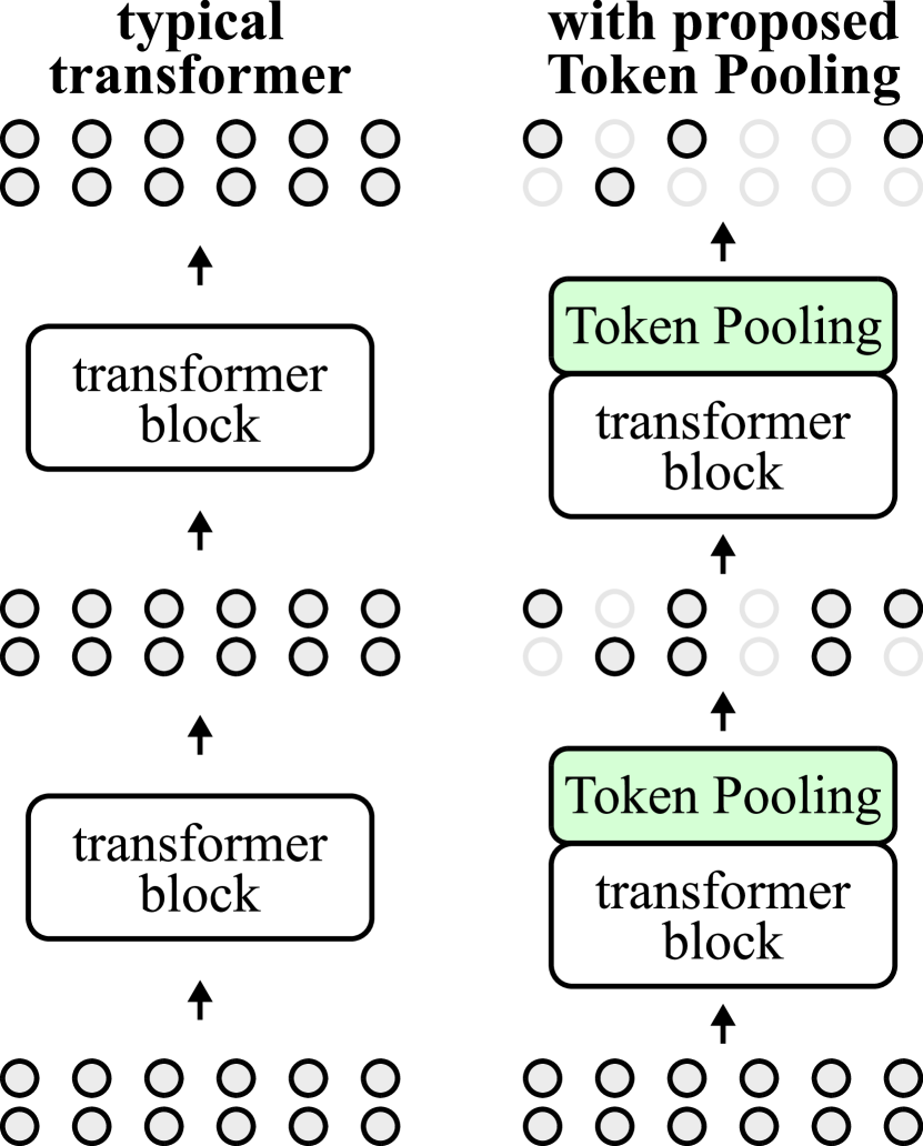
(a) Proposed Token Pooling

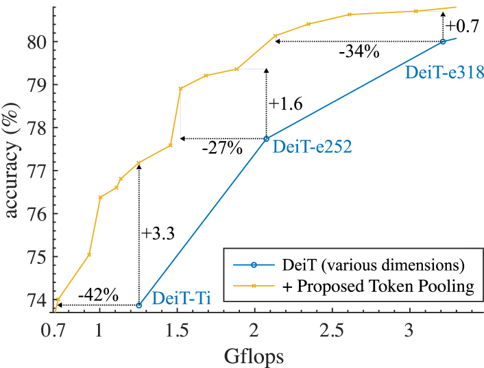
(b) Accuracy vs. computation

(c) Token Pooling via cluster analysis of token representations.

Figure 1: (a) We propose Token Pooling, a novel token downsampling method, for visual transformers. (b) The proposed method achieves a state-of-the-art trade-off between accuracy and computation. (c) Token Pooling uses cluster analysis to aggregate information from individual tokens automatically. We show the input images and the token clusters at the 6-th layer of DeiT-S.

Contributions.

The paper makes the following contributions:

• We conduct an extensive study of prior downsampling techniques for visual transformers by comparing their computation-accuracy trade-offs.

• We analyze the computational cost of vision-transformer components and the limitations of the prior score-based downsampling methods. We also show that attention layers behave like low-pass filtering and thus produce redundant tokens.

• Motivated by the redundancy in images and features, we propose a novel token downsampling technique, Token Pooling, for transformers via error minimization and achieve a significant improvement in the computation-accuracy trade-off.

2 Related work

In this section, we introduce vision transformers, and review existing methods that improve the efficiency of transformers including existing token-downsampling methods.

2.1 Vision transformers

Vision transformers (Dosovitskiy et al., 2020; Touvron et al., 2021; Heo et al., 2021; Liu et al., 2021; Pan et al., 2021) utilize the transformer architecture that is originally designed for NLP by Vaswani et al. (2017) and further popularized by Radford et al. (2018) and Devlin et al. (2019). In a high level, a vision transformer is a composition of $L$ transformer blocks that take a set of input tokens and return another set of output tokens. In vision, input tokens are features representing individual non-overlapping image patches. To perform classification, a classification token is inserted to estimate the probabilities of individual classes. To achieve the state-of-the-art, ViT (Dosovitskiy et al., 2020) used pretraining on JFT-300M, a proprietary dataset much larger than standard ImageNet1k (Deng et al., 2009). Recently, DeiT (Touvron et al., 2021) achieved state-of-the-art results with advanced training on ImageNet1k only.

Let the set of tokens at depth $l$ be ${\mathcal{F}}^{l}=\{{\bm{f}}^{l}_{0},\dots,{\bm{f}}^{l}_{N}\}$ where ${\bm{f}}^{l}_{i}\in\mathbb{R}^{M}$ is the feature values of the $i$-th token. A typical transformer block $\phi$ at depth $l$ processes ${\mathcal{F}}^{l}$ by a Multi-head Self-Attention (MSA) layer and a point-wise Multi-Layer Perceptron (MLP). Let matrix ${\bm{F}}\in\mathbb{R}^{N\times M}$ be a row-wise concatenation of tokens ${\mathcal{F}}^{l}$. Then,

$$\phi({\bm{F}}) \;=\;\operatorname{MLP}(\operatorname{MSA}({\bm{F}}))\;\;\;\;\;\;\text{such that}$$ (1)

$$\operatorname{MSA}({\bm{F}}) \;=\;[{\bm{O}}_{1},{\bm{O}}_{2},\dots,{\bm{O}}_{H}]{\bm{W}}^{O}$$ (2)

where $H$ is the number of heads, matrix ${\bm{W}}^{O}\in\mathbb{R}^{M\times M}$ is a learnable parameter of the block, $[,]$ is column-wise concatenation and ${\bm{O}}_{h}\in\mathbb{R}^{N\times d}$ is the output of $h$-th attention head for $d=M/H$:

$${\bm{O}}_{h} ={\bm{A}}_{h}{\bm{V}}_{h}\;\;\;\text{ such that }\;\;\;{\bm{A}}_{h}=\operatorname{softmax}({\bm{Q}}_{h}{\bm{K}}_{h}^{\top}{\big{/}}\sqrt{d})\in\mathbb{R}^{N\times N}.$$ (3)

Keys ${\bm{K}}_{h}$, queries ${\bm{Q}}_{h}$ and values ${\bm{V}}_{h}$ are linear projections of the input tokens (QKV projections):

$${\bm{Q}}_{h} ={\bm{F}}{\bm{W}}_{h}^{Q},\;\;\;\;{\bm{K}}_{h}={\bm{F}}{\bm{W}}_{h}^{K},\;\;\;\;{\bm{V}}_{h}={\bm{F}}{\bm{W}}_{h}^{V}$$ (4)

where ${\bm{W}}_{h}^{Q}\in\mathbb{R}^{M\times d}$, ${\bm{W}}_{h}^{K}\in\mathbb{R}^{M\times d}$, ${\bm{W}}_{h}^{V}\in\mathbb{R}^{M\times d}$ are learnable linear transformations. Note, the number of tokens is not affected by the transformer blocks, $|{\mathcal{F}}^{l+1}|=|{\mathcal{F}}^{l}|$.

2.2 Efficient transformers

Similar to many machine learning models, the efficiency of transformers can be improved via meta-parameter search (Howard et al., 2017; Tan & Le, 2019), automated neural architecture search (Elsken et al., 2019; Tan et al., 2019; Wu et al., 2019), manipulating the input size and resolution of feature maps (Paszke et al., 2016; Howard et al., 2017; Zhao et al., 2018), pruning (LeCun et al., 1990), quantization (Jacob et al., 2018), and sparsification (Gale et al., 2019), . For example, Dosovitskiy et al. (2020) and Touvron et al. (2021) obtain a family of ViT and DeiT models, respectively, by varying the input resolution, the number of heads $H$, and the feature dimensionality $M$. Each of the models operates with a different computational requirement and accuracy. In the following, we review techniques developed for transformers.

2.2.1 Efficient self-attention

The softmax-attention layer (3) has a quadratic time complexity w.r.t. the number of tokens, $\mathcal{O}(N^{2})$. In many NLP applications where every token represents a word or a character, $N$ can be large, making attention a computation bottleneck (Dai et al., 2019; Rae et al., 2019). While many works improve the time complexity of attention layers, as we will see in § 3.1, they are not the bottleneck in most current vision transformers.

The time complexity of an attention layer can be reduced by restricting the attention field-of-view and thus imposing sparsity on ${\bm{A}}_{h}$ in (3). This can be achieved using the spatial relationship between tokens in the image/text domain (Parmar et al., 2018; Ramachandran et al., 2019; Qiu et al., 2020; Beltagy et al., 2020; Child et al., 2019; Zaheer et al., 2020) or based on token values using locality-sensitive hashing, sorting, compression, (Kitaev et al., 2020; Roy et al., 2021; Vyas et al., 2020; Tay et al., 2020a; Liu et al., 2018; Wang et al., 2020; Tay et al., 2021). Prior works have also proposed attention mechanisms with lower time complexity, $\mathcal{O}(N)$ or $\mathcal{O}(N\log N)$ (Katharopoulos et al., 2020; Peng et al., 2021; Choromanski et al., 2021; Tay et al., 2021).

Note that the goal of these methods is to reduce the time complexity of the attention layer—the number of tokens remains the same across the transformer blocks. In contrast, our method reduces the number of tokens after attention has been computed. Thereby, we can utilize these methods to further improve the overall efficiency of transformers.

Recently, Wu et al. (2020) proposed a new attention-based layer that learns a small number of query vectors to extract information from the input feature map. Similarly, Wu et al. (2021) replace self-attention with a new recurrent layer that outputs a smaller number of tokens. In comparison, our method directly minimizes the token reconstruction error due to token downsampling. Also, our layer has no learnable parameters and can be easily incorporated into existing vision transformers.

2.2.2 Downsampling methods for transformers

Grid-downsampling.

The input tokens of the first vision transformer block are computed from image patches. Therefore, even though transformers treat tokens as a set, we can still associate a grid to the tokens using their initial locations on the image. The regular grid structure allows typical downsampling methods, such as max/mean pooling, uniform sub-sampling. For example, Liu et al. (2021); Heo et al. (2021) use convolutions with stride to downsample the feature maps formed by the tokens. Also, these works increase the feature dimensionality with depth, similarly to CNNs.

Score-based token downsampling.

In the area of NLP, Goyal et al. (2020) introduce the idea of dropping tokens. Their approach, called PoWER-BERT, is based on a measure of significance score, which is defined as the total attention given to a token from all other tokens. Specifically, the significance scores of all tokens in the $l$-th transformer block, $\bm{s}^{l}\in\mathbb{R}^{N}$, is computed by

$$\bm{s}^{l}=\sum_{h=1}^{H}{{\bm{A}}_{h}^{l}}^{\top}{\bm{1}},$$ (5)

where ${\bm{A}}_{h}^{l}$ is the attention weights of head $h$ defined in (3). They only pass $K_{l}$ tokens with the highest scores in $\bm{s}^{l}$ to the next transformer block. The pruning is performed on all blocks.

PoWER-BERT is trained using a three-stage process. First, given a base architecture, they pretrain a model without pruning. In the second stage, a soft-selection layer is inserted after each transformer block, and the model is finetuned for a small number of epochs. Once learned, the number of tokens to keep, $K_{l}$, for each layer is computed from the soft-selection layers. Last, the model is finetuned again with the tokens pruned using the $K_{l}$ from the second stage. See Goyal et al. (2020) for details.

Recently, Rao et al. (2021) proposed Dynamic-ViT that also uses scores to prune tokens. Unlike PoWER-BERT, which computes significance scores from attention weights, Rao et al. use a dedicated sub-network with learned parameters. The method requires knowledge distillation, Gumbel-Softmax, and straight-through estimators on top of the DeiT training.

We will analyze the limitations of score-based methods in § 3.2.

3 Analysis

This section addresses three questions. First, it identifies the computational bottleneck of vision transformers. Second, it discusses the limitations of score-based downsampling. Third, it analyzes how the softmax-attention affects the redundancy in tokens.

3.1 Computation analysis of vision transformers

Layer Complexity Computation ($10^{9}$ Flops) ViT-B/384 ($N=577$) ViT-B ($N=197$) DeiT-S ($N=197$) DeiT-Ti ($N=197$) softmax-attention ${\mathcal{O}}(LN^{2}M)$ 6.18 0.72 0.36 0.18 QKV projections ${\mathcal{O}}(LNM^{2})$ 12.25 4.18 1.05 0.26 O projection ${\mathcal{O}}(LNM^{2})$ 4.08 1.39 0.35 0.09 Multi-linear Perceptron ${\mathcal{O}}(LNM^{2})$ 32.67 11.15 2.79 0.70 Total ${\mathcal{O}}(LNM(M+N))$ 55.5 17.6 4.6 1.3

Table 1: Time complexity and computation breakdown of ViT (Dosovitskiy et al., 2020) and DeiT (Touvron et al., 2021). $L$ is the number of transformer blocks, $N$ is the number of input tokens (patches), and $M$ is the feature dimensionality. All models take input images of size $224\times 224$ except ViT-B/384, which uses $384\times 384$. The softmax-attention layers constitute a fraction (15% or less) of the total compute, whereas fully-connected layers (MLP and projections) spend over 80%.

We analyze the time complexity and computational costs (measured in flops) of commonly used vision transformers, namely ViT and DeiT. We breakdown the computation into four categories: softmax-attention (3), QKV projections (4), O projection (2) and MLP (1). As shown in Table 1, in all these vision transformers, the main computational bottleneck is the fully-connected layers that spend over 80% of the total computation. In comparison, softmax-attention only takes less than 15%. Note that we explicitly break down the multi-head attention into the softmax-attention, QKV and O projections, as they have different time complexity, see Table 1. This decomposition reveals that the QKV and O projections spend most of the computations of the multi-head self-attention.

3.2 Limitations of score-based token downsampling

Existing score-based token downsampling methods like PoWER-BERT and Dynamic-ViT utilize scoring functions to determine the tokens to keep (or prune). They keep tokens with the top-K scores and discard the rest. Since these scoring functions are continuous with limited Lipschitz constants, tokens that are close in the feature space will be assigned similar scores. Therefore, these similar tokens will likely either be all kept or discarded, as illustrated in 3(a). As our experiments show, this redundancy (in the kept tokens) and severe information loss (in the pruned tokens) deteriorate the computation-accuracy trade-off of the score-based downsampling methods.

(a) Score-based downsampling

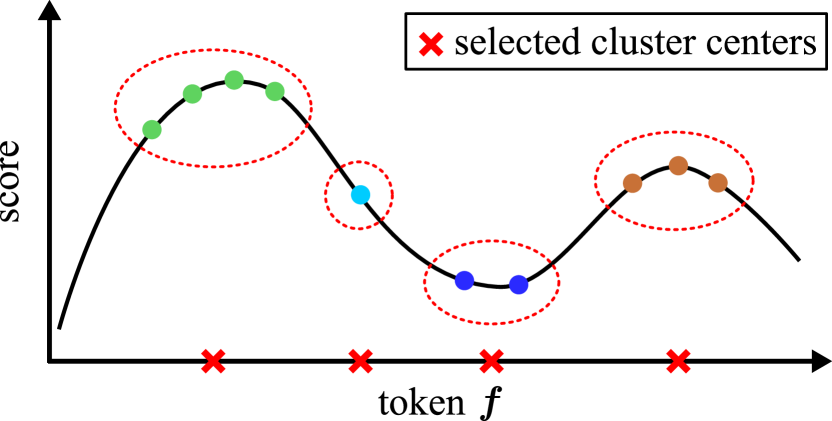
(b) Proposed downsampling

Figure 3: Score-based downsampling methods (Goyal et al., 2020; Rao et al., 2021) vs. our method. In the figure, the x-axis represents the token values (in one dimension), and the y-axis represents their scores. Suppose four tokens are to be selected. (a) Score-based methods select tokens with higher scores. Since the scoring function is continuous, all tokens in the left lobe will be selected, resulting in redundancy and information loss in the right lobe. (b) The proposed method first forms four clusters to approximate the set of tokens, then selects the cluster centers. Thus, the output tokens are a more accurate representation of the original token set than the score-based methods.

3.3 Attention as a low-pass filter

Given a query vector ${\bm{q}}$, a set of key vectors $\mathcal{K}=\{{\bm{k}}_{1},\dots,{\bm{k}}_{N}\}$, the corresponding value vectors $\mathcal{V}=\{{\bm{v}}_{1},\dots,{\bm{v}}_{N}\}$ and a scalar $\alpha>0$, softmax-attention computes the output via

$${\bm{o}}({\bm{q}})=\frac{1}{z({\bm{q}})}\sum_{i=1}^{N}\exp(\alpha\,{\bm{q}}\cdot{\bm{k}}_{i})\,{\bm{v}}_{i} z({\bm{q}})=\sum_{i=1}^{N}\exp(\alpha\,{\bm{q}}\cdot{\bm{k}}_{i}).$$ where (6)

Note that we write ${\bm{o}}({\bm{q}})$ to indicate that the output vector ${\bm{o}}$ is a function of the query ${\bm{q}}$. If the query vector and all key vectors are normalized to have a fixed $\ell^{2}$ norm, we can rewrite (6) as

$${\bm{o}}({\bm{q}}) =\frac{1}{z^{\prime}({\bm{q}})}\!\sum_{i=1}^{N}\exp\!\left(-\frac{\alpha}{2}\|{\bm{q}}-{\bm{k}}_{i}\|^{2}\right){\bm{v}}_{i}=\frac{1}{z^{\prime}({\bm{q}})}\!\int\!\exp\!\left(-\frac{\alpha}{2}\|{\bm{q}}-{\bm{k}}\|^{2}\right)\!\left(\sum_{i=1}^{N}\!\delta({\bm{k}}-{\bm{k}}_{i}){\bm{v}}_{i}\right)\differential{{\bm{k}}}$$

$$=\frac{1}{z^{\prime}({\bm{q}})}\ G\!\left({\bm{q}};\frac{1}{\alpha}\right)*S({\bm{q}};\mathcal{K},\mathcal{V})$$ (7)

where $*$ represents high-dimensional convolution, $z^{\prime}({\bm{q}})=\sum_{i}\exp(-\frac{\alpha}{2}\|{\bm{q}}-{\bm{k}}_{i}\|^{2})=G\!\left({\bm{q}};\frac{1}{\alpha}\right)*S({\bm{q}};\mathcal{K},1)$ is the normalization scalar function, $G\!\left({\bm{q}};\sigma^{2}\right)=\exp({-\|{\bm{q}}\|^{2}}\big{/}{2\sigma^{2}})$ is an isometric Gaussian kernel, and $S({\bm{q}};\mathcal{K},\mathcal{V})=\sum_{i=1}^{N}\delta({\bm{q}}-{\bm{k}}_{i})\,{\bm{v}}_{i}$ is a high-dimensional sparse signal, which is composed of $N$ delta functions located at ${\bm{k}}_{i}$ with value ${\bm{v}}_{i}$. According to (7), given query vectors ${\bm{q}}_{1},\dots,{\bm{q}}_{N}$, there are two conceptual steps to compute softmax-attention:

1. filter $S({\bm{q}};\mathcal{K},\mathcal{V})$ with a Gaussian kernel to get ${\bm{o}}({\bm{q}})$, and

2. sample ${\bm{o}}({\bm{q}})$ at coordinates ${\bm{q}}_{1},\dots,{\bm{q}}_{N}$ to get the output vectors ${\bm{o}}_{1},\dots,{\bm{o}}_{N}$.

Since Gaussian filtering is low-pass, ${\bm{o}}({\bm{q}})$ is a smooth signal. Therefore, the output tokens of the attention layer, discrete samples of ${\bm{o}}({\bm{q}})$, contain similar feature values. So, based on Nyquist-Shannon sampling theorem (Shannon, 1949), there exists redundant information in the output, which is used by our methods to reduce computation without losing much of the important information.

Note that our analysis is based on the normalized query and key vectors, which can be achieved by inserting a normalizing layer before the softmax-attention layer without significantly affecting the performance of a transformer, as shown by Kitaev et al. (2020). It has also been empirically observed by Goyal et al. (2020) and Rao et al. (2021) that even without the normalization, transformers produce tokens with similar values. To demonstrate this, in all our experiments, we use standard multi-head attention without normalizing keys and queries. We conduct an ablation study with normalized keys and queries in Appendix F.

4 Token pooling

Pruning tokens inevitably loses information. In this section, we formulate a new token downsampling principle enabling strategical tokens selection that preserves the most information. Based on this principle, we formulate and discuss several Token Pooling algorithms.

Given a set of output tokens ${\mathcal{F}}=\{{\bm{f}}_{1},\dots,{\bm{f}}_{N}\}$ of a transformer block, our goal is to find a smaller set of tokens $\hat{{\mathcal{F}}}=\{\hat{{\bm{f}}}_{1},\dots,\hat{{\bm{f}}}_{K}\}$ that after upsampling minimizes the reconstruction error of ${\mathcal{F}}$. Specifically, the reconstruction of $u({\bm{f}}_{i};\hat{{\mathcal{F}}})$ of token ${\bm{f}}_{i}$ is computed via interpolating the tokens in $\hat{{\mathcal{F}}}$. The reconstruction error is then defined as

$$\ell({\mathcal{F}},\hat{{\mathcal{F}}})=\sum_{{\bm{f}}_{i}\in{\mathcal{F}}}\|{\bm{f}}_{i}-u({\bm{f}}_{i};\hat{{\mathcal{F}}})\|^{2}.$$ (8)

To simplify our formulation and reduce computation, we use nearest-neighbor interpolation as $u$. As a consequence, the reconstruction error (8) becomes

$$\ell({\mathcal{F}},\hat{{\mathcal{F}}})=\sum_{{\bm{f}}_{i}\in F}\ \min_{\hat{{\bm{f}}}_{j}\in\hat{F}}\ \|{\bm{f}}_{i}-\hat{{\bm{f}}}_{j}\|^{2},$$ (9)

which is the asymmetric Chamfer divergence between ${\mathcal{F}}$ and $\hat{{\mathcal{F}}}$ (Barrow et al., 1977; Mechrez et al., 2018). The loss (9) can be minimized by the K-Means algorithm, clustering the tokens in ${\mathcal{F}}$ into $K$ clusters.

The proposed Token Pooling layer is defined in Algorithm 1. It downsamples input tokens via clustering the tokens and returns the cluster centers (the average of the tokens in a cluster). As we have shown above, this operation directly minimizes the reconstruction error (9) caused by the downsampling. Intuitively, clustering the tokens provides a more accurate and diverse representation of the original set of tokens, compared to the top-K selection used by score-based downsampling methods, as shown in 3(b). Note that Token Pooling is robust to the initialization of cluster centers, as shown in Appendix B. Below, we provide details of the clustering algorithms.

K-Means.

We use the K-Means algorithm to minimize (9) via the following iterations:

$$a(i) \;\;\;\leftarrow\;\;\;\arg\min_{j}\|{\bm{f}}_{i}-\hat{\bm{f}}_{j}\| \forall i\in\{1,2,\dots,N\}$$ (10)

$$\hat{\bm{f}}_{j} \;\;\;\leftarrow\;\;\;\sum_{i=1}^{N}[a(i)=j]{\bm{f}}_{i}\Bigg{/}\sum_{i=1}^{N}[a(i)=j] \forall j\in\{1,2,\dots,K\}$$ (11)

where $[\,]$ is the Iverson bracket and $a$ is the cluster assignment function. The overall algorithm complexity is ${\mathcal{O}}(TKNM)$ where $T$ is the number of iterations. The vast majority of the computation is spent on the repetitive evaluation of the distances between tokens and centroids in step (10).

K-Medoids.

We can use the more efficient K-Medoids algorithm by replacing step (11) with:

$$n(j)\;\leftarrow\;{\arg\min_{i:a(i)=j}\sum_{i^{\prime}:a(i^{\prime})=j}\|{\bm{f}}_{i}-{\bm{f}}_{i^{\prime}}\|^{2}} \hat{\bm{f}}_{j}\;\leftarrow\;{\bm{f}}_{n(j)}.$$ and (12)

These steps minimize objective (9) under the medoid constraint: $\hat{\mathcal{F}}\subseteq{\mathcal{F}}$.

The advantage of the K-Medoids algorithm is its time complexity ${\mathcal{O}}(TKN+N^{2}M)$, which is substantially lower in practice as we only compute the distances between tokens once. In our experience, it requires less than 5 iterations to converge. Apart from the distance matrix computation, the cost of the K-Medoids algorithm is negligible when compared with the cost of the other layers.

input : tokens ${\mathcal{F}}=\{{\bm{f}}_{1},\dots,{\bm{f}}_{N}\}$; target set size $K$; (optional) weights ${\mathcal{W}}=\{w_{1},\dots,w_{N}\}$

output : downsampled set $\hat{\mathcal{F}}=\{\hat{\bm{f}}_{1},\dots,\hat{\bm{f}}_{K}\}$

1 if $k\geq N$ then return F;

2 initialize cluster centers $\hat{\mathcal{F}}$ to be the $K$ tokens from ${\mathcal{F}}$ with the highest weights ;

3 while not converged and max number of iterations is not reached do

4       for  $i\in\{1,...,N\}$  do  update cluster assignment $z(i)\leftarrow\arg\min_{j=1}^{K}\|{\bm{f}}_{i}-\hat{\bm{f}}_{j}\|$ ;

5       for  $j\in\{1,...,K\}$  do  update cluster center $\hat{{\bm{f}}}_{j}$ according to the chosen clustering algorithm, that is either (11), (12), (15) or (18) ;

6      

return weighted means of tokens in each cluster

Algorithm 1 Token Pooling

Weighted clustering.

Reconstruction error (9) treats every token equally; however, each token contributes differently to the final output of an attention layer. Thus, we also consider a weighted reconstruction error: $\ell({\mathcal{F}},\hat{{\mathcal{F}}};{\bm{w}})=\sum_{{\bm{f}}_{i}\in F}\min_{\hat{{\bm{f}}}_{j}\in\hat{F}}w_{i}\|{\bm{f}}_{i}-\hat{{\bm{f}}}_{j}\|^{2}$ where ${\bm{w}}=[w_{1},\dots,w_{N}]$ are the positive weights corresponding to the individual tokens in ${\mathcal{F}}$. Appendix A details the clustering algorithms for the weighted case. A good choice of the weights is the significance scores (5), $w_{i}=s_{i}$. The significance score identifies the tokens that influence the current transformer block most and thus should be approximated more precisely.

5 Experiments

Our implementation is based on DeiT (Touvron et al., 2021) where we insert downsampling layers after each transformer block. To evaluate the pure effect of downsampling, we keep all meta-parameters of DeiT, including the feature dimensionality, network depth, learning rate schedule, . We also do not use knowledge distillation during training. We use ImageNet1k classification benchmark (Russakovsky et al., 2015). Our cost and performance metrics are flops and top-1 accuracy.

Methods.

We evaluate the following token downsampling methods:

1. Convolution downsampling. We implement uniform grid-downsampling via convolution with stride 2, , the tokens corresponding to the adjacent image patches are concatenated and mapped to $\mathbb{R}^{M}$. This design is used in Liu et al. (2021); Heo et al. (2021). See details in Appendix D.

2. PoWER-BERT. We implement PoWER-BERT on DeiT, following (Goyal et al., 2020).

3. Random selection, a simple baseline randomly selecting $K$ tokens without replacement.

4. Importance selection chooses $K$ tokens by drawing from a categorical distribution without replacement with probabilities proportional to the significance score (5) of each token.

5. Token Pooling use K-Means or K-Medoids algorithms, or their weighted versions, WK-Means or WK-Medoids, respectively. The weights are the significance scores (5).

Selection of ${\bm{K}}=[K_{1},\dots,K_{L}]$.

To fairly compare our Token Pooling with PoWER-BERT and other baselines, all methods (except convolution downsampling) use the same number of retained tokens for downsampling layers. Appendix C details the selection of ${\bm{K}}$.

Training protocol.

(1) A base DeiT model (DeiT-S) is trained using the original training (Touvron et al., 2021). (2) We then finetune the base DeiT model using the second stage of PoWER-BERT’s training and acquire ${\bm{K}}$. (3) We further finetune the downsampling methods using ${\bm{K}}$. (4) We also finetune the base DeiT model. Our protocol ensures a fair comparison such that all of the models are trained with the same number of iterations, the same learning rate schedule, .

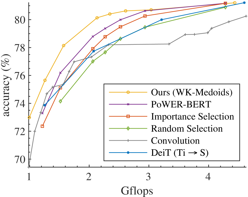
(a) Models based on DeiT-S

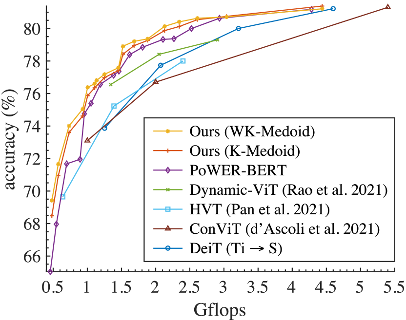
(b) Comparison with current SOTA

Figure 4: Main results. (a) shows the accuracy when we apply different downsampling methods to DeiT-S. More is in Appendix G. (b) shows a comparison between the proposed method with the state-of-the-art downsampling methods. The results of our method and PoWER-BERT are acquired by varying ${\bm{K}}$ and the base architecture among DeiT-Ti, DeiT-e252, DeiT-e318, and DeiT-S.

5.1 Main results

First, we apply different downsampling methods on DeiT-S. As shown in 4(a), random selection achieves a similar trade-off as lowering feature dimensionality $M$. While convolution with stride is better than adjusting $M$ at the low-compute regime, it fails in high-compute regimes. Importance selection improves upon random selection but is still outperformed by PoWER-BERT. Our Token Pooling (with weighted K-Medoids) achieves the best trade-off in all regimes.

Next, we apply Token Pooling to DeiT models with different $M$ (DeiT-Ti, DeiT-e252, DeiT-e318, and DeiT-S). Figure 5 shows trade-off curves for each DeiT model. Token Pooling enables each of the models to achieve a better computation-accuracy trade-off than simply varying the feature dimensionality $M$. For each computational budget, we find the combination of $M$ and ${\bm{K}}$ that gives the highest accuracy. The best balance is achieved by applying Token Pooling and selecting the best $M$. We do the same for PoWER-BERT. 4(b) shows the results of the proposed Token Pooling and state-of-the-art methods. We cite the results of Rao et al. (2021), d’Ascoli et al. (2021), and Pan et al. (2021). Our Token Pooling achieves the best accuracy across all evaluated compute regimes.

Finally, we compare the best computation-accuracy trade-off achieved by Token Pooling (with WK-Medoids and varying $M$) with standard DeiT models in 1(b). As can be seen, utilizing Token Pooling, we significantly improve the computation costs of DeiT-Ti by 42% and improve the top-1 accuracy by 3.3 points at the same flops. Similar benefits can be seen on DeiT-e252 and DeiT-e318.

5.2 Ablation studies

6(a) compares methods utilizing significance scores. As can be seen, using importance selection improves upon the simple random selection. By minimizing the reconstruction error (9), our method achieves better cost-accuracy trade-off. 6(b) evaluates Token Pooling with different clustering algorithms. Weighted versions outperform regular versions of K-Means and K-Medoids. Due to the higher time complexity, K-Means is outperformed by K-Medoids (the curves are shifted toward the right). See the metrics and flops used by clustering in table format in Appendix G. Still, all Token Pooling variants outperform the baseline, demonstrating the effectiveness of our method.

More ablation studies are in the appendices, including the effect of cluster-center initialization (Appendix B), results of convolution downsampling (Appendix D), results of Token Pooling before finetuning (Appendix E), results with normalized keys and queries of softmax attention (Appendix F), and detailed information (${\bm{K}}$, flops, accuracy, clustering cost) of our models (Appendix G).

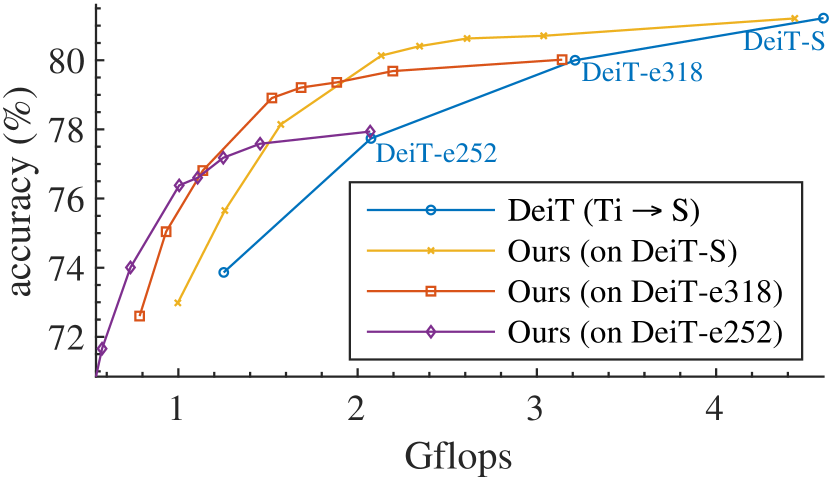
Figure 5: The figure shows the results when we apply Token Pooling to various DeiT architectures. Token Pooling consistently improves the computation-accuracy trade-off for all evaluated architectures. By utilizing both Token Pooling and architecture search, we can further improve the accuracy at a given flops budget. For example, at 1 Gflop, we should use Token Pooling on DeiT-e252 instead of DeiT-S.

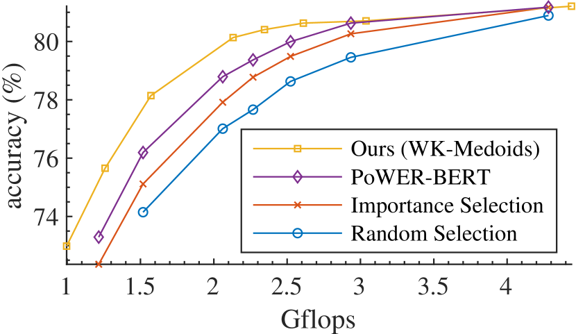
(a) Ours vs. methods using significance score

(b) Variants of Token Pooling

Figure 6: Ablation studies of (a) downsampling methods using significance score, and (b) proposed Token Pooling using different clustering algorithms. The base model is DeiT-S for all methods.

6 Conclusions

This paper provides two insights of vision transformers: first, their computational bottleneck is the fully-connected layers, and second, attention layers generate redundant representations due to the connection to Gaussian filtering. Token Pooling, our novel nonuniform data-aware downsampling operator, utilizes these insights and significantly improves the computation-accuracy balance of DeiT, compared to existing downsampling techniques. We believe that Token Pooling is a timely development and can be used with other techniques (architecture search, quantization) to spur the design of efficient vision transformers.

Appendix A Weighted clustering algorithms

Weighted K-Means

minimizes the following objective w.r.t. $\hat{\mathcal{F}}=\{\hat{{\bm{f}}}_{1},\dots,\hat{{\bm{f}}}_{K}\}\subset\mathbb{R}^{M}$:

$$\ell({\mathcal{F}},\hat{{\mathcal{F}}})=\sum_{{\bm{f}}_{i}\in F}\ \min_{\hat{{\bm{f}}}_{j}\in\hat{F}}w_{i}\|{\bm{f}}_{i}-\hat{{\bm{f}}}_{j}\|^{2}$$ (13)

The extension of the K-Means algorithm to the weighted case iterates the following steps:

$$a(i) \;\;\;\leftarrow\;\;\;\arg\min_{j}\|{\bm{f}}_{i}-\hat{\bm{f}}_{j}\| \forall i\in\{1,2,\dots,N\},$$ (14)

$$\hat{\bm{f}}_{j} \;\;\;\leftarrow\;\;\;\frac{\sum_{i=1}^{N}[a(i)=j]w_{i}{\bm{f}}_{i}}{\sum_{i=1}^{N}[a(i)=j]w_{i}} \forall j\in\{1,2,\dots,K\}.,$$ (15)

Weighted K-Medoids

optimizes objective (13) under the medoid constraint $\hat{\mathcal{F}}\subset{\mathcal{F}}$:

$$a(i) \;\;\;\leftarrow\;\;\;\arg\min_{j}\|{\bm{f}}_{i}-\hat{\bm{f}}_{j}\| \forall i\in\{1,2,\dots,N\},$$ (16)

$$n(j) \;\;\;\leftarrow\;\;\;\operatornamewithlimits{\arg\min}_{i:\,z(i)=j}\sum_{i^{\prime}:\,a(i^{\prime})=j}\|{\bm{f}}_{i}-{\bm{f}}_{i^{\prime}}\|^{2} \forall j\in\{1,2,\dots,K\},$$ (17)

$$\hat{\bm{f}}_{j} \;\;\;\leftarrow\;\;\;{\bm{f}}_{n(j)}.$$ (18)

Appendix B Clustering initialization ablations

We examine the effect of the cluster center initialization. We compare our default initialization, which uses the tokens with top-K significance scores as initial cluster centers, with random initialization, which randomly selects tokens as initial cluster centers. As shown in Figure 7, Token Pooling is robust to the initialization methods.

Figure 7: Default initialization vs. random initialization. Our Token Pooling is robust to initialization of clustering algorithms. The default initialization is top-K w.r.t. significance score, see Algorithm 1.

Appendix C Training details

To fairly compare PoWER-BERT and the baseline methods with the proposed Token Pooling, all methods (except convolution downsampling) use the same target number of tokens for downsampling layers after each transformer block. Specifically, we run the second stage of the PoWER-BERT training for 30 epochs with various values of the token-selection weight parameter producing a family of models. Each of the models has a different number of retained tokens at each of its $L$ transformer blocks: ${\bm{K}}=(K_{1},\dots,K_{L})$. Appendix G lists all combinations of ${\bm{K}}$. We then finetune the base DeiT model (from the first stage training of PoWER-BERT) with the selected ${\bm{K}}$ using the third (last) stage of PoWER-BERT, random selection, importance selection or our Token Pooling using the same ${\bm{K}}$.

We find that the DeiT models provided by Touvron et al. (2021) are under-fit, and their accuracy improves with additional training, see Figure 8. After the standard DeiT training, we restart the training. This ensures that downsampling models and DeiT with almost the same amount of training.

Figure 8: This figure shows the results of the pretrained DeiT models provided by Touvron et al. (2021) (DeiT) and the DeiT models trained with our protocol (DeiT-2x). Our training protocal uses the same hyper-parameters provided by Touvron et al. (2021), but after the model is trained, we finetune the model using the same hyper-parameters (restart the learning rate schedule). We also show DeiT-Distil results (cited from (Touvron et al., 2021)), which use knowledge distillation.

Appendix D Convolution downsampling

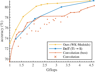
Figure 9: Results of convolution downsampling

As mentioned in the main paper, we enumerate combinations of layers to insert the convolution downsampling layer. We use 2x2 convolution with stride 2 like in Liu et al. (2021). To keep the feature dimensionality of DeiT the same (and evaluate the pure effect of the downsampling layers), the output feature dimensionality is the same as the input. With 196 tokens in DeiT-S model, we can include no more than 3 convolution downsampling layers as each layer reduces the number of token by a factor of 4. When using 3 layers at depths $l_{1}<l_{2}<l_{3}$, we restrict $l_{2}-l_{1}=l_{3}-l_{2}$. With these constraints, we enumerate all possible downsampling configurations. Each of the combinations produces a model with a different computation-accuracy trade-off, and we report the Pareto front, , the best accuracy these models achieve at a given flop. See Figure 9.

Appendix E Results without finetuning

Since Token Pooling minimizes the reconstruction error due to token downsampling, in this section, we evaluate the performance when we insert Token Pooling layers into a pre-trained model without finetuning. Figure 10 shows the results when we directly insert Token Pooling layers (using the same downsampling ratios in 6(b)) into a pretrained DeiT-S. As can be seen, minimizing the reconstruction error, Token Pooling preserves information that enables the model to retain accuracy during token downsampling.

In Figure 10, we also show the results when we replace tokens to their cluster centers (WK-Means, carry, no finetuning and WK-Medoids, carry, no finetuning). Specifically, in addition to outputting $K$ cluster centers, we count the number of tokens assigned to a cluster center and carry the count when we compute softmax-attention in the next transformer blocks. This operation preserves the attention weights, and since the models are not trained after inserting Token Pooling layers, it preserves the most accuracy. In practice, when the models are trained with Token Pooling layers, the carry operation is not important.

Figure 10: The figure shows the performance results when we insert Token Pooling layers into a pretrained DeiT-S without finetuning the model (skip step 3 of the training protocol in Section 5).

Appendix F Normalized key and query vectors

Our analysis of softmax-attention in § 3.3 assumes the query and the key vectors are normalized to have a constant $\ell^{2}$ norm. It has been observed by Kitaev et al. (2020) that normalizing key and query vectors does not change the performance of a transformer. Thus, for all experiments, we train models without the norm normalization. In this section, we verify this observation by training various DeiT, PoWER-BERT, and Token Pooling with normalized keys and queries. We found that the scalar $\alpha$ in the softmax attention layer (6) can affect the performance of a transformer with normalized keys and queries. As can be seen in 11(a), setting the scalar $\alpha=1$ slightly deteriorates the performance of the model. Instead of using a fixed $\alpha$, we let the model learn the $\alpha$ for each layer. As can be seen in 11(b), learning $\alpha$ enables the resulting models to achieve similar cost-accuracy trade-off as the standard (unnormalized) models. With or without the normalization and the learnable $\alpha$, the proposed Token Pooling significantly improves the cost-accuracy trade-off of DeiT and outperforms PoWER-BERT.

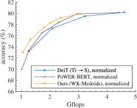
(a) $\alpha=1$

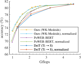
(b) Learned $\alpha$ for each layer

Figure 11: Results of models using normalized key and query vectors with (a) $\alpha=1$ and (b) learned $\alpha$ in (6). The base model architecture is DeiT-S.

Appendix G Clustering algorithm ablations

Tables 3–2 detail the results of PoWER-BERT and Token Pooling on the DeiT architectures that we tested (DeiT-S, DeiT-e318, and DeiT-e252). Figure 12 shows the results. Table 2 details the results of the best cost-accuracy trade-off achieved by the proposed Token Pooling (using K-Medoids and WK-Medoids) and PoWER-BERT via varying token sparsity and feature dimensionality of DeiT.

Apart from the standard K-Means and K-Medoids, other clustering approaches could be used. Many methods are not suitable due to efficiency constraints. For example, normalized cut (Shi & Malik, 2000) uses expensive spectral methods. One prerequisite of using K-Means and K-Medoids is the number of clusters, $K$. While selecting $K$ for each of the layers may be tedious and difficult, one can choose $K$ via computational budgets and heuristics. In this work, we use the automatic search procedure proposed by Goyal et al. (2020) to determine $K$, see Appendix C.

Since both K-Means and K-Medoids require specifying the number of clusters $K$ in advance, one may consider using methods automatically determining $K$. Nevertheless, such methods typically have other parameters, which are less interpretable than $K$. For example, mean-shift (Cheng, 1995) or quick-shift (Vedaldi & Soatto, 2008) require specifying the kernel size. From our experience, determining these parameters is challenging. Also, since the number of clusters (and hence the number of output tokens) is determined on the fly during inference, the computational requirement can fluctuate, making deployment of these models difficult.

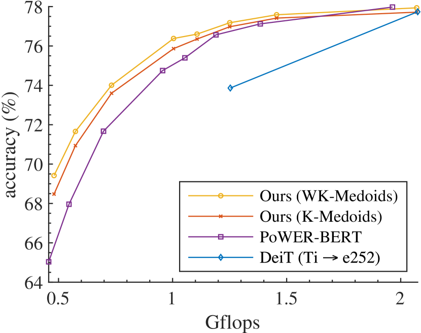
(a) DeiT-e252 as the base architecture

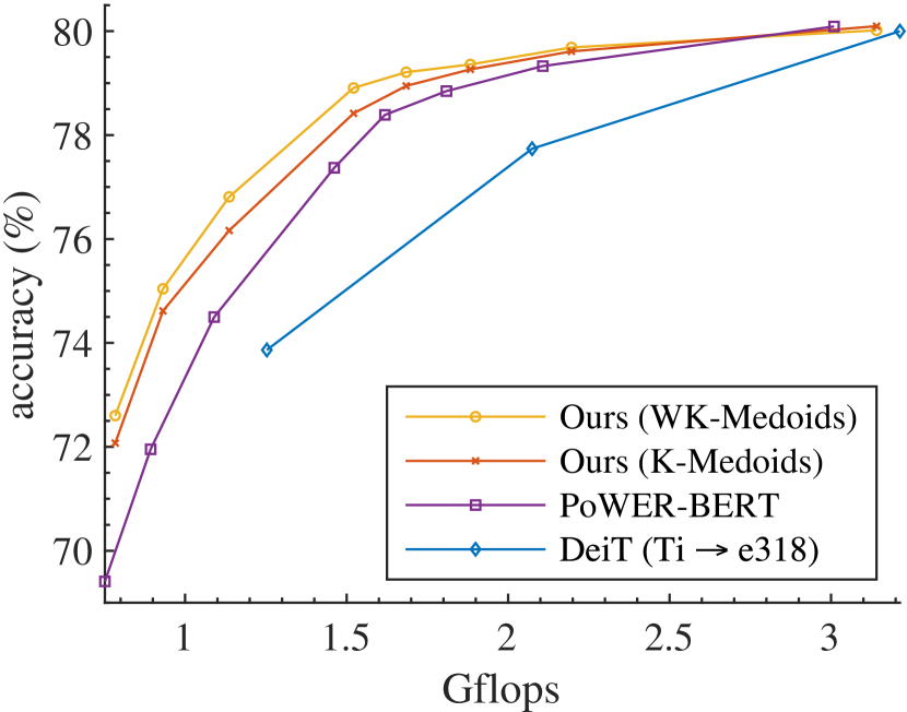
(b) DeiT-e318 as the base architecture

Figure 12: This figure compares the cost-accuracy curves of Token Pooling with PoWER-BERT using (a) DeiT-e252 and (b) DeiT-e318 as the base architectures.

DeiT (Ti $\rightarrow$ S) PoWER-BERT Token Pooling (K-Medoids) Token Pooling (WK-Medoids) Gflops Accuracy (%) Gflops Accuracy (%) Gflops Accuracy (%) Gflops Accuracy (%) - - 0.46 65.0 0.48 68.5 0.48 69.4 - - 0.55 68.0 0.57 70.9 0.57 71.7 - - 0.70 71.7 0.73 73.6 0.73 74.0 - - 0.89 72.0 0.93 74.6 0.93 75.0 - - 0.96 74.8 1.00 75.9 1.00 76.4 - - 1.05 75.4 1.11 76.4 1.11 76.6 1.25 73.9 1.19 76.6 1.25 77.0 1.25 77.2 - - 1.38 77.1 1.46 77.4 1.46 77.6 - - 1.46 77.4 1.52 78.4 1.52 78.9 - - 1.62 78.4 1.68 78.9 1.68 79.2 2.07 77.7 1.81 78.8 1.88 79.3 1.88 79.4 - - 2.11 79.3 2.13 79.9 2.13 80.1 - - 2.27 79.4 2.35 80.1 2.35 80.4 - - 2.52 80.0 2.61 80.5 2.61 80.6 3.21 80.0 2.93 80.6 3.04 80.7 3.04 80.7 4.60 81.2 4.28 81.2 4.44 81.4 4.44 81.2

Table 2: Best cost-accuracy trade-off achieved by PoWER-BERT and the proposed Token Pooling via varying sparsity level and feature dimensionality.

clustering method Weighting ImageNet Accuracy GFlops Sparsity level 0: $\bm{K}=[196,196,195,194,189,180,173,173,173,173,173,173]$ PoWER-BERT N/A 81.2 4.3 K-Means 81.3 4.7 (+0.4) ✓ 81.1 4.7 (+0.4) K-Medoids 81.4 4.4 (+0.1) ✓ 81.2 4.4 (+0.1) Sparsity level 1: $\bm{K}=[196,195,193,188,169,140,121,110,73,38,7,0]$ PoWER-BERT N/A 80.6 2.9 K-Means 80.7 3.3 (+0.4) ✓ 80.8 3.3 (+0.4) K-Medoids 80.7 3.0 (+0.1) ✓ 80.7 3.0 (+0.1) Sparsity level 2: $\bm{K}=[196,195,190,177,141,108,84,69,35,18,3,0]$ PoWER-BERT N/A 80.0 2.5 K-Means 80.5 2.8 (+0.3) ✓ 80.5 2.8 (+0.3) K-Medoids 80.5 2.6 (+0.1) ✓ 80.6 2.6 (+0.1) Sparsity level 3: $\bm{K}=[196,194,187,163,118,85,58,47,20,12,2,0]$ PoWER-BERT N/A 79.4 2.3 K-Means 80.1 2.5 (+0.2) ✓ 80.4 2.5 (+0.2) K-Medoids 80.1 2.3 (+0.08) ✓ 80.4 2.3 (+0.08) Sparsity level 4: $\bm{K}=[196,193,179,142,97,64,46,34,13,9,1,0]$ PoWER-BERT N/A 78.8 2.1 K-Means 79.8 2.3 (+0.2) ✓ 80.0 2.3 (+0.2) K-Medoids 79.9 2.1 (+0.07) ✓ 80.1 2.1 (+0.07) Sparsity level 5: $\bm{K}=[194,183,142,89,41,20,10,7,0,0,0,0]$ PoWER-BERT N/A 76.2 1.5 K-Means 77.6 1.7 (+0.2) ✓ 78.1 1.7 (+0.2) K-Medoids 77.8 1.6 (+0.05) ✓ 78.1 1.6 (+0.05) Sparsity level 6: $\bm{K}=[186,162,102,56,13,4,2,2,0,0,0,0]$ PoWER-BERT N/A 73.3 1.2 K-Means 75.0 1.4 (+0.2) ✓ 75.6 1.4 (+0.2) K-Medoids 75.4 1.3 (+0.04) ✓ 75.7 1.3 (+0.04) Sparsity level 7: $\bm{K}=[162,129,66,33,4,1,1,0,0,0,0,0]$ PoWER-BERT N/A 69.6 1.0 K-Means 72.4 1.1 (+0.1) ✓ 73.0 1.1 (+0.1) K-Medoids 72.3 1.0 (+0.03) ✓ 73.0 1.0 (+0.03)

Table 3: Results of applying Token Pooling and PoWER-BERT on DeiT-S model. The models are grouped by ${\bm{K}}$ described in Appendix C. The integer list denotes the maximal number of tokens retained after each transformer block. These numbers do not take into account the classification token, which is always retained. Thus, “0” means that only the classification token remains. Additional flops (denoted by the parentheses) are due to clustering.

clustering method Weighting ImageNet Accuracy GFlops Sparsity level 0: $\bm{K}=[196,196,196,194,192,184,181,181,170,170,170,170]$ PoWER-BERT N/A 80.1 3.0 K-Medoids 80.1 3.1 (+0.1) ✓ 80.0 3.1 (+0.1) Sparsity level 1: $\bm{K}=[196,195,195,190,171,147,132,122,66,43,15,0]$ PoWER-BERT N/A 79.3 2.1 K-Medoids 79.6 2.2 (+0.1) ✓ 79.7 2.2 (+0.1) Sparsity level 2: $\bm{K}=[196,195,193,180,143,109,92,77,40,21,4,0]$ PoWER-BERT N/A 78.8 1.8 K-Medoids 79.3 1.9 (+0.09) ✓ 79.4 1.9 (+0.09) Sparsity level 3: $\bm{K}=[196,195,190,165,119,84,65,50,26,14,3,0]$ PoWER-BERT N/A 78.3 1.6 K-Medoids 78.9 1.7 (+0.07) ✓ 79.2 1.7 (+0.07) Sparsity level 4: $\bm{K}=[196,194,184,149,97,65,47,33,12,9,2,0]$ PoWER-BERT N/A 77.4 1.5 K-Medoids 78.4 1.5 (+0.06) ✓ 78.9 1.5 (+0.06) Sparsity level 5: $\bm{K}=[196,186,153,93,40,15,12,9,0,0,0,0]$ PoWER-BERT N/A 74.5 1.1 K-Medoids 76.2 1.1 (+0.05) ✓ 76.8 1.1 (+0.05) Sparsity level 6: $\bm{K}=[193,173,109,52,16,4,4,4,0,0,0,0]$ PoWER-BERT N/A 72.0 0.89 K-Medoids 74.6 0.93 (+0.04) ✓ 75.0 0.93 (+0.04) Sparsity level 7: $\bm{K}=[183,145,80,33,5,1,1,2,0,0,0,0]$ PoWER-BERT N/A 69.4 0.75 K-Medoids 72.1 0.78 (+0.03) ✓ 72.6 0.78 (+0.03)

Table 4: Results of applying Token Pooling and PoWER-BERT on DeiT-e318 model. The models are grouped by ${\bm{K}}$ described in Appendix C. The integer list denotes the maximal number of tokens retained after each transformer block. These numbers do not take into account the classification token, which is always retained. Thus, “0” means that only the classification token remains. Additional flops (denoted by the parentheses) are due to clustering.

clustering method Weighting ImageNet Accuracy GFlops Sparsity level 0: $\bm{K}=[196,196,196,195,193,189,177,177,177,177,177,177]$ PoWER-BERT N/A 78.0 2.0 K-Medoids 77.7 2.1 (+0.1) ✓ 77.9 2.1 (+0.1) Sparsity level 1: $\bm{K}=[196,196,195,189,176,161,123,122,76,48,17,0]$ PoWER-BERT N/A 77.1 1.4 K-Medoids 77.4 1.5 (+0.07) ✓ 77.6 1.5 (+0.07) Sparsity level 2: $\bm{K}=[196,196,193,179,154,123,88,79,39,22,5,0],$ PoWER-BERT N/A 76.6 1.2 K-Medoids 77.0 1.3 (+0.06) ✓ 77.2 1.3 (+0.06) Sparsity level 3: $\bm{K}=[196,195,188,167,131,96,63,52,13,11,2,0],$ PoWER-BERT N/A 75.4 1.1 K-Medoids 76.4 1.1 (+0.05) ✓ 76.6 1.1 (+0.05) Sparsity level 4: $\bm{K}=[196,194,181,147,111,75,48,36,5,7,2,0]$ PoWER-BERT N/A 74.8 0.96 K-Medoids 75.9 1.0 (+0.04) ✓ 76.4 1.0 (+0.04) Sparsity level 5: $\bm{K}=[196,187,129,88,54,20,10,10,0,1,0,0]$ PoWER-BERT N/A 71.7 0.70 K-Medoids 73.6 0.73 (+0.03) ✓ 74.0 0.73 (+0.03) Sparsity level 6: $\bm{K}=[194,163,83,44,22,6,1,3,0,0,0,0]$ PoWER-BERT N/A 68.0 0.55 K-Medoids 70.9 0.57 (+0.02) ✓ 71.7 0.57 (+0.02) Sparsity level 7: $\bm{K}=[188,122,58,28,12,2,0,2,0,0,0,0]$ PoWER-BERT N/A 65.0 0.46 K-Medoids 68.5 0.48 (+0.02) ✓ 69.4 0.48 (+0.02)

Table 5: Results of applying Token Pooling and PoWER-BERT on DeiT-e252 model. The models are grouped by ${\bm{K}}$ described in Appendix C. The integer list denotes the maximal number of tokens retained after each transformer block. These numbers do not take into account the classification token, which is always retained. Thus, “0” means that only the classification token remains. Additional flops (denoted by the parentheses) are due to clustering.

References

- Barrow et al. (1977) Harry G Barrow, Jay M Tenenbaum, Robert C Bolles, and Helen C Wolf. Parametric correspondence and chamfer matching: Two new techniques for image matching. Technical report, SRI International Menlo Park CA Artificial Intelligence Center, 1977.
- Belfor et al. (1994) Ricardo AF Belfor, Marc PA Hesp, Reginald L Lagendijk, and Jan Biemond. Spatially adaptive subsampling of image sequences. Transactions on Image Processing, 3:492–500, 1994.
- Beltagy et al. (2020) Iz Beltagy, Matthew E. Peters, and Arman Cohan. Longformer: The long-document transformer. arXiv:2004.05150, 2020.
- Cheng (1995) Yizong Cheng. Mean shift, mode seeking, and clustering. IEEE Transactions on Pattern Analysis and Machine Intelligence (PAMI), 17(8):790–799, 1995.
- Child et al. (2019) Rewon Child, Scott Gray, Alec Radford, and Ilya Sutskever. Generating long sequences with sparse transformers. arXiv preprint arXiv:1904.10509, 2019.
- Choromanski et al. (2021) Krzysztof Choromanski, Valerii Likhosherstov, David Dohan, Xingyou Song, Andreea Gane, Tamas Sarlos, Peter Hawkins, Jared Davis, Afroz Mohiuddin, Lukasz Kaiser, et al. Rethinking attention with performers. International Conference on Learning Representations (ICLR), 2021.
- Dai et al. (2019) Zihang Dai, Zhilin Yang, Yiming Yang, Jaime G Carbonell, Quoc Le, and Ruslan Salakhutdinov. Transformer-XL: Attentive language models beyond a fixed-length context. In Proceedings of the 57th Annual Meeting of the Association for Computational Linguistics, pp. 2978–2988, 2019.
- d’Ascoli et al. (2021) Stéphane d’Ascoli, Hugo Touvron, Matthew Leavitt, Ari Morcos, Giulio Biroli, and Levent Sagun. ConViT: Improving vision transformers with soft convolutional inductive biases. International Conference on Machine Learning (ICML), 2021.
- Deng et al. (2009) Jia Deng, Wei Dong, Richard Socher, Li-Jia Li, Kai Li, and Li Fei-Fei. ImageNet: A large-scale hierarchical image database. In IEEE Conference on Computer Vision and Pattern Recognition (CVPR), pp. 248–255, 2009.
- Devlin et al. (2019) Jacob Devlin, Ming-Wei Chang, Kenton Lee, and Kristina Toutanova. BERT: Pre-training of deep bidirectional transformers for language understanding. In Proceedings of the 2019 Conference of the North American Chapter of the Association for Computational Linguistics: Human Language Technologies, Volume 1 (Long and Short Papers), pp. 4171–4186, 2019.
- Dosovitskiy et al. (2020) Alexey Dosovitskiy, Lucas Beyer, Alexander Kolesnikov, Dirk Weissenborn, Xiaohua Zhai, Thomas Unterthiner, Mostafa Dehghani, Matthias Minderer, Georg Heigold, Sylvain Gelly, et al. An image is worth 16x16 words: Transformers for image recognition at scale. In International Conference on Learning Representations (ICLR), 2020.
- Elsken et al. (2019) Thomas Elsken, Jan Hendrik Metzen, and Frank Hutter. Neural architecture search: A survey. The Journal of Machine Learning Research, 20(1):1997–2017, 2019.
- Gale et al. (2019) Trevor Gale, Erich Elsen, and Sara Hooker. The state of sparsity in deep neural networks. arXiv preprint arXiv:1902.09574, 2019.
- Goyal et al. (2020) Saurabh Goyal, Anamitra Roy Choudhury, Saurabh Raje, Venkatesan Chakaravarthy, Yogish Sabharwal, and Ashish Verma. PoWER-BERT: Accelerating BERT inference via progressive word-vector elimination. In International Conference on Machine Learning (ICML), pp. 3690–3699, 2020.
- Heo et al. (2021) Byeongho Heo, Sangdoo Yun, Dongyoon Han, Sanghyuk Chun, Junsuk Choe, and Seong Joon Oh. Rethinking spatial dimensions of vision transformers. In IEEE International Conference on Computer Vision (ICCV), 2021.
- Howard et al. (2017) Andrew G Howard, Menglong Zhu, Bo Chen, Dmitry Kalenichenko, Weijun Wang, Tobias Weyand, Marco Andreetto, and Hartwig Adam. MobileNets: Efficient convolutional neural networks for mobile vision applications. arXiv preprint arXiv:1704.04861, 2017.
- Ilharco et al. (2020) Gabriel Ilharco, Cesar Ilharco, Iulia Turc, Tim Dettmers, Felipe Ferreira, and Kenton Lee. High performance natural language processing. In Proceedings of the 2020 Conference on Empirical Methods in Natural Language Processing: Tutorial Abstracts, pp. 24–27, 2020.
- Jacob et al. (2018) Benoit Jacob, Skirmantas Kligys, Bo Chen, Menglong Zhu, Matthew Tang, Andrew Howard, Hartwig Adam, and Dmitry Kalenichenko. Quantization and training of neural networks for efficient integer-arithmetic-only inference. In IEEE Conference on Computer Vision and Pattern Recognition (CVPR), pp. 2704–2713, 2018.
- Katharopoulos et al. (2020) Angelos Katharopoulos, Apoorv Vyas, Nikolaos Pappas, and François Fleuret. Transformers are RNNs: Fast autoregressive transformers with linear attention. In International Conference on Machine Learning (ICML), pp. 5156–5165, 2020.
- Kitaev et al. (2020) Nikita Kitaev, Lukasz Kaiser, and Anselm Levskaya. Reformer: The efficient transformer. In International Conference on Learning Representations (ICLR), 2020.
- LeCun et al. (1990) Yann LeCun, John S Denker, and Sara A Solla. Optimal brain damage. In Advances in Neural Information Processing Systems (NeurIPS), pp. 598–605, 1990.
- Liu et al. (2018) Peter J. Liu, Mohammad Saleh, Etienne Pot, Ben Goodrich, Ryan Sepassi, Lukasz Kaiser, and Noam Shazeer. Generating wikipedia by summarizing long sequences. In International Conference on Learning Representations (ICLR), 2018.
- Liu et al. (2021) Ze Liu, Yutong Lin, Yue Cao, Han Hu, Yixuan Wei, Zheng Zhang, Stephen Lin, and Baining Guo. Swin transformer: Hierarchical vision transformer using shifted windows. arXiv preprint arXiv:2103.14030, 2021.
- Marin et al. (2019) Dmitrii Marin, Zijian He, Peter Vajda, Priyam Chatterjee, Sam Tsai, Fei Yang, and Yuri Boykov. Efficient segmentation: Learning downsampling near semantic boundaries. In IEEE International Conference on Computer Vision (ICCV), pp. 2131–2141, 2019.
- Marvasti (2012) Farokh Marvasti. Nonuniform Sampling: Theory and Practice. Springer Science & Business Media, 2012.
- Mechrez et al. (2018) Roey Mechrez, Itamar Talmi, Firas Shama, and Lihi Zelnik-Manor. Maintaining natural image statistics with the contextual loss. In Asian Conference on Computer Vision (ACCV), pp. 427–443, 2018.
- Pan et al. (2021) Zizheng Pan, Bohan Zhuang, Jing Liu, Haoyu He, and Jianfei Cai. Scalable visual transformers with hierarchical pooling. IEEE International Conference on Computer Vision (ICCV), 2021.
- Parmar et al. (2018) Niki Parmar, Ashish Vaswani, Jakob Uszkoreit, Lukasz Kaiser, Noam Shazeer, Alexander Ku, and Dustin Tran. Image transformer. In International Conference on Machine Learning (ICML), pp. 4055–4064. PMLR, 2018.
- Paszke et al. (2016) Adam Paszke, Abhishek Chaurasia, Sangpil Kim, and Eugenio Culurciello. ENet: A deep neural network architecture for real-time semantic segmentation. arXiv preprint arXiv:1606.02147, 2016.
- Peng et al. (2021) Hao Peng, Nikolaos Pappas, Dani Yogatama, Roy Schwartz, Noah Smith, and Lingpeng Kong. Random feature attention. In International Conference on Learning Representations (ICLR), 2021.
- Qiu et al. (2020) Jiezhong Qiu, Hao Ma, Omer Levy, Wen-tau Yih, Sinong Wang, and Jie Tang. Blockwise self-attention for long document understanding. In Proceedings of the 2020 Conference on Empirical Methods in Natural Language Processing: Findings, pp. 2555–2565, 2020.
- Rabbani (2002) Majid Rabbani. JPEG2000: Image compression fundamentals, standards and practice. Journal of Electronic Imaging, 11(2):286, 2002.
- Radford et al. (2018) Alec Radford, Karthik Narasimhan, Tim Salimans, and Ilya Sutskever. Improving language understanding by generative pre-training. 2018. URL https://s3-us-west-2.amazonaws.com/openai-assets/research-covers/language-unsupervised/language_understanding_paper.pdf.
- Rae et al. (2019) Jack W Rae, Anna Potapenko, Siddhant M Jayakumar, Chloe Hillier, and Timothy P Lillicrap. Compressive transformers for long-range sequence modelling. In International Conference on Learning Representations (ICLR), 2019.
- Ramachandran et al. (2019) Prajit Ramachandran, Niki Parmar, Ashish Vaswani, Irwan Bello, Anselm Levskaya, and Jon Shlens. Stand-alone self-attention in vision models. 32, 2019.
- Rao et al. (2021) Yongming Rao, Wenliang Zhao, Benlin Liu, Jiwen Lu, Jie Zhou, and Cho-Jui Hsieh. DynamicViT: Efficient vision transformers with dynamic token sparsification. ArXiv, abs/2106.02034, 2021.
- Recasens et al. (2018) Adria Recasens, Petr Kellnhofer, Simon Stent, Wojciech Matusik, and Antonio Torralba. Learning to zoom: a saliency-based sampling layer for neural networks. In European Conference on Computer Vision (ECCV), pp. 51–66, 2018.
- Roy et al. (2021) Aurko Roy, Mohammad Saffar, Ashish Vaswani, and David Grangier. Efficient content-based sparse attention with routing transformers. Transactions of the Association for Computational Linguistics, 9:53–68, 2021.
- Russakovsky et al. (2015) Olga Russakovsky, Jia Deng, Hao Su, Jonathan Krause, Sanjeev Satheesh, Sean Ma, Zhiheng Huang, Andrej Karpathy, Aditya Khosla, Michael Bernstein, et al. ImageNet large scale visual recognition challenge. International Journal of Computer Vision (IJCV), 115(3):211–252, 2015.
- Shannon (1949) Claude E Shannon. Communication in the presence of noise. Proceedings of the IRE, 37(1):10–21, jan 1949. doi: 10.1109/jrproc.1949.232969. URL https://doi.org/10.1109/jrproc.1949.232969.
- Shi & Malik (2000) Jianbo Shi and Jitendra Malik. Normalized cuts and image segmentation. IEEE Transactions on Pattern Analysis and Machine Intelligence (PAMI), 22(8):888–905, 2000.
- Tan & Le (2019) Mingxing Tan and Quoc Le. EfficientNet: Rethinking model scaling for convolutional neural networks. In International Conference on Machine Learning (ICML), pp. 6105–6114, 2019.
- Tan et al. (2019) Mingxing Tan, Bo Chen, Ruoming Pang, Vijay Vasudevan, Mark Sandler, Andrew Howard, and Quoc V Le. MnasNet: Platform-aware neural architecture search for mobile. In IEEE Conference on Computer Vision and Pattern Recognition (CVPR), pp. 2820–2828, 2019.
- Tay et al. (2020a) Yi Tay, Dara Bahri, Liu Yang, Donald Metzler, and Da-Cheng Juan. Sparse sinkhorn attention. In International Conference on Machine Learning (ICML), pp. 9438–9447, 2020a.
- Tay et al. (2020b) Yi Tay, Mostafa Dehghani, Dara Bahri, and Donald Metzler. Efficient transformers: A survey. arXiv preprint arXiv:2009.06732, 2020b.
- Tay et al. (2021) Yi Tay, Dara Bahri, Donald Metzler, Da-Cheng Juan, Zhe Zhao, and Che Zheng. Synthesizer: Rethinking self-attention in transformer models. International Conference on Machine Learning (ICML), 2021.
- Touvron et al. (2021) Hugo Touvron, Matthieu Cord, Matthijs Douze, Francisco Massa, Alexandre Sablayrolles, and Hervé Jégou. Training data-efficient image transformers & distillation through attention. pp. 10347–10357, 2021.
- Unat et al. (2009) Didem Unat, Theodore Hromadka, and Scott B Baden. An adaptive sub-sampling method for in-memory compression of scientific data. In Data Compression Conference, pp. 262–271. IEEE, 2009.
- Vaswani et al. (2017) Ashish Vaswani, Noam Shazeer, Niki Parmar, Jakob Uszkoreit, Llion Jones, Aidan N Gomez, Łukasz Kaiser, and Illia Polosukhin. Attention is all you need. Advances in Neural Information Processing Systems (NeurIPS), 30:5998–6008, 2017.
- Vedaldi & Soatto (2008) Andrea Vedaldi and Stefano Soatto. Quick shift and kernel methods for mode seeking. In European Conference on Computer Vision (ECCV), pp. 705–718, 2008.
- Vyas et al. (2020) Apoorv Vyas, Angelos Katharopoulos, and François Fleuret. Fast transformers with clustered attention. Advances in Neural Information Processing Systems (NeurIPS), 33, 2020.
- Wang et al. (2020) Sinong Wang, Belinda Li, Madian Khabsa, Han Fang, and Hao Ma. Linformer: Self-attention with linear complexity. arXiv preprint arXiv:2006.04768, 2020.
- Wu et al. (2019) Bichen Wu, Xiaoliang Dai, Peizhao Zhang, Yanghan Wang, Fei Sun, Yiming Wu, Yuandong Tian, Peter Vajda, Yangqing Jia, and Kurt Keutzer. FBNet: Hardware-aware efficient ConvNet design via differentiable neural architecture search. In IEEE Conference on Computer Vision and Pattern Recognition (CVPR), pp. 10734–10742, 2019.
- Wu et al. (2020) Bichen Wu, Chenfeng Xu, Xiaoliang Dai, Alvin Wan, Peizhao Zhang, Zhicheng Yan, Masayoshi Tomizuka, Joseph Gonzalez, Kurt Keutzer, and Peter Vajda. Visual transformers: Token-based image representation and processing for computer vision. arXiv preprint arXiv:2006.03677, 2020.
- Wu et al. (2021) Lemeng Wu, Xingchao Liu, and Qiang Liu. Centroid transformers: Learning to abstract with attention. arXiv preprint arXiv:2102.08606, 2021.
- Zaheer et al. (2020) Manzil Zaheer, Guru Guruganesh, Avinava Dubey, Joshua Ainslie, Chris Alberti, Santiago Ontanon, Philip Pham, Anirudh Ravula, Qifan Wang, Li Yang, et al. Big bird: Transformers for longer sequences. Advances in Neural Information Processing Systems (NeurIPS), 2020.
- Zhao et al. (2018) Hengshuang Zhao, Xiaojuan Qi, Xiaoyong Shen, Jianping Shi, and Jiaya Jia. ICNet for real-time semantic segmentation on high-resolution images. In European Conference on Computer Vision (ECCV), pp. 405–420, 2018.
- Zheng et al. (2021) Sixiao Zheng, Jiachen Lu, Hengshuang Zhao, Xiatian Zhu, Zekun Luo, Yabiao Wang, Yanwei Fu, Jianfeng Feng, Tao Xiang, Philip HS Torr, et al. Rethinking semantic segmentation from a sequence-to-sequence perspective with transformers. In IEEE Conference on Computer Vision and Pattern Recognition (CVPR), pp. 6881–6890, 2021.