Full-frequency dynamical Bethe-Salpeter equation without frequency and a study of double excitations

Abstract

The Bethe-Salpeter equation (BSE) that results from the GW approximation to the self-energy is a frequency-dependent (nonlinear) eigenvalue problem due to the dynamically screened Coulomb interaction between electrons and holes. The computational time required for a numerically exact treatment of this frequency dependence is $O(N^{6})$, where $N$ is the system size. To avoid the common static screening approximation, we show that the full-frequency dynamical BSE can be exactly reformulated as a frequency-independent eigenvalue problem in an expanded space of single and double excitations. When combined with an iterative eigensolver and the density fitting approximation to the electron repulsion integrals, this reformulation yields a dynamical BSE algorithm whose computational time is $O(N^{5})$, which we verify numerically. Furthermore, the reformulation provides direct access to excited states with dominant double excitation character, which are completely absent in the spectrum of the statically screened BSE. We study the $2^{1}A_{\mathrm{g}}$ state of butadiene, hexatriene, and octatetraene and find that GW/BSE overestimates the excitation energy by about 1.5–2 eV and significantly underestimates the double excitation character.

The Bethe-Salpeter equation (BSE) is an exact relation between the two-particle Green’s function and the one-particle self-energy. Using the GW approximation to the self-energy yields an approximate solution of the BSE, providing neutral excitation energies and spectra. Hedin (1965); Strinati (1988) Due to its success in solids, Hanke and Sham (1980); Strinati (1984); Albrecht et al. (1998); Rohlfing and Louie (2000) the BSE has been increasingly applied to molecules Tiago and Chelikowsky (2005); Faber et al. (2014); Körbel et al. (2014); Bruneval, Hamed, and Neaton (2015); Jacquemin, Duchemin, and Blase (2015); Rangel et al. (2017); Blase et al. (2020) and compared to common quantum chemistry methods like time-dependent density functional theory (TDDFT), the algebraic diagrammatic construction (ADC), and coupled-cluster theory. Jacquemin et al. (2016); Jacquemin, Duchemin, and Blase (2017); Blase, Duchemin, and Jacquemin (2018); Gui, Holzer, and Klopper (2018) Physically, the BSE modifies the GW energy gaps due to electron-hole interactions Hanke and Sham (1980); Rohlfing and Louie (2000). Importantly, the electron-hole attraction in the BSE is screened, which is the primary difference compared to time-dependent Hartree-Fock (HF) theory.

In terms of spatial molecular orbitals, the BSE is a frequency-dependent eigenvalue problem $\bm{\mathcal{A}}(\Omega)\mathbf{X}=\Omega\mathbf{X}$ where

$$\mathcal{A}_{ia,jb}(\Omega) =A_{ia,jb}-K^{\mathrm{(p)}}_{abij}(\Omega)$$ (1a)

$$A_{ia,jb} =(E_{a}-E_{i})\delta_{ij}\delta_{ab}+\kappa(ia|jb)-(ab|ij),$$ (1b)

$E_{p}$ are GW quasiparticle energies, $(pq|rs)$ are electron repulsion integrals in $(11|22)$ notation, and $\kappa=2$ for a singlet excited state and $0$ for a triplet excited state. Here and throughout, we make the Tamm-Dancoff approximation (TDA), which typically introduces negligible error and removes triplet instabilities Rangel et al. (2017); Blase, Duchemin, and Jacquemin (2018) but can cause significant errors when plasmonic effects (collective electronic excitations) are important.Rocca, Lu, and Galli (2010) Furthermore, we use $i,j,k,l$ to index orbitals that are occupied in the mean-field reference; $a,b,c,d$ to index orbitals that are unoccupied; and $p,q,r,s$ to index general orbitals. For simplicity, we assume real orbitals.

Like the self-energy in the GW approximation, the polarizable part of the direct electron-hole interaction requires a frequency integration,

$$\begin{split}&K^{(\mathrm{p})}_{abij}(\Omega)=\frac{i}{2\pi}\int d\omega e^{-i\omega 0+}W^{\mathrm{(p)}}_{abij}(\omega)\\ &\times\Bigg{[}\frac{1}{\Omega-\omega-(E_{b}-E_{i})+i\eta}+\frac{1}{\Omega+\omega-(E_{a}-E_{j})+i\eta}\Bigg{]},\end{split}$$ (2)

where

$$W^{(\mathrm{p})}_{abij}(\omega)=\int d{\bm{r}}_{1}d{\bm{r}}_{2}\phi_{a}({\bm{r}}_{1})\phi_{b}({\bm{r}}_{1})W^{(\mathrm{p})}({\bm{r}}_{1},{\bm{r}}_{2};\omega)\phi_{i}({\bm{r}}_{2})\phi_{j}({\bm{r}}_{2})$$ (3)

are matrix elements of the polarizable part of the screened Coulomb interaction

$$W^{(\mathrm{p})}({\bm{r}}_{1},{\bm{r}}_{2};\omega)=\int d{\bm{r}}\varepsilon^{-1}({\bm{r}}_{1},{\bm{r}};\omega)|{\bm{r}}-{\bm{r}}_{2}|^{-1}-|{\bm{r}}_{1}-{\bm{r}}_{2}|^{-1}.$$ (4)

In practice, this frequency integration is typically avoided by making the static screening approximation Krause and Klopper (2017); Bruneval et al. (2016); Liu et al. (2020); Rocca, Lu, and Galli (2010),

$$K_{abij}^{\text{(p)}}(\Omega)\approx W_{abij}^{\text{(p)}}(\omega=0).$$ (5)

Although computationally convenient, the static screening approximation often introduces errors of about 0.1-0.3 eV Rohlfing and Louie (2000); Ma, Rohlfing, and Molteni (2009); Loos and Blase (2020). Moreover, the static screening approximation significantly reduces the number of excited states predicted by the BSE; in particular, as will be discussed more later, it removes double excitations from the BSE spectrum Romaniello et al. (2009); Elliott et al. (2011); Authier and Loos (2020); Loos and Blase (2020). In this work, we show that full-frequency dynamical BSE calculations can be performed by diagonalizing a frequency-independent Hamiltonian matrix in an expanded space of single and double excitations (“full-frequency” means that a model dielectric function or plasmon-pole approximationRohlfing and Louie (2000) is not used, and “dynamical” means that the static screening approximation is not used). This formulation enables the use of iterative eigensolvers and provides access to BSE eigenvectors with dominant double excitation character, which allows us to assess the quality of double excitations predicted by the GW/BSE approach.

As the most common example, we will consider the use of the random-phase approximation (RPA) to calculate the screened Coulomb interaction. Like in our previous work Bintrim and Berkelbach (2021), we consider screening within the TDA to the RPA, which avoids technical problems associated with positive and negative eigenvalue pairs in the RPA matrix; the impact of this choice will be assessed with numerical tests, reported below. Within the TDA, the RPA eigenproblem is $\mathbf{S}\bm{X}^{m}=\Omega_{m}\bm{X}^{m}$, where $S_{ia,jb}=(\varepsilon_{a}-\varepsilon_{i})\delta_{ab}\delta_{ij}+2(ia|bj)$. Using the spectral representation of the RPA polarizability, the frequency integration (LABEL:eq:freq_int) can be performed analytically to give

$$\begin{split}&K^{(\mathrm{p})}_{abij}(\Omega)=2\sum_{m}^{\Omega_{m}>0}(ij|\rho_{m})(ab|\rho_{m})\\ &\hskip 20.00003pt\times\Bigg{[}\frac{1}{\Omega-(E_{b}-E_{i})-\Omega_{m}}+\frac{1}{\Omega-(E_{a}-E_{j})-\Omega_{m}}\Bigg{]},\end{split}$$ (6)

where $(pq|\rho_{m})=\sum_{ia}X_{ia}^{m}(pq|ia)$ and we have dropped $i\eta$ terms. The severe disadvantage of the above expression is that it requires an explicit enumeration of the $O(N^{2})$ excitations entering into the polarizability, which requires diagonalizing the RPA or TDA matrix with $O(N^{6})$ cost. Unsurprisingly, given their similar structure, the same problem plagues full-frequency implementations of the GW approximation. van Setten et al. (2015)

Here we show that the dynamical BSE (1), with the frequency dependence appearing as a sum of simple poles as in Eq. (LABEL:eq:Kd), can be obtained by downfolding a larger, frequency-independent matrix. This is analogous to what was done in our previous work on the GW approximation Bintrim and Berkelbach (2021). First, let us assume that the GW eigenvalues $E_{p}$ have been computed. In that case, it is reasonably straightforward to show that the self-consistent eigenvalues of $\bm{\mathcal{A}}(\Omega)$ are the same as those of the frequency-independent matrix

$$\bm{\mathcal{H}}=\left(\begin{array}[]{ccc}\mathbf{A}&-\mathbf{V}^{\text{e}}&-\mathbf{V}^{\text{h}}\\ \mathbf{(V^{\text{h}})^{\dagger}}&\mathbf{D}&\mathbf{0}\\ \mathbf{(V^{\text{e}})^{\dagger}}&\mathbf{0}&\mathbf{D}\end{array}\right),$$ (7)

where

$$\mathbf{D} =[-\bm{E}_{\text{occ}}]\oplus\bm{E}_{\text{vir}}\oplus\mathbf{S}$$ (8a)

$$V^{\text{h}}_{ia,ldkc} =\sqrt{2}(il|kc)\delta_{ad}$$ (8b)

$$V^{\text{e}}_{ia,ldkc} =\sqrt{2}(kc|ad)\delta_{il}.$$ (8c)

Note that the orbital energies $\varepsilon_{p}$ in Eq. (8b) are the mean-field orbital energies, e.g. from DFT, and $\mathbf{S}$ is the direct RPA matrix in the TDA. The matrix (7) can be expressed in a basis of single and double excitations, similar to configuration interaction or coupled-cluster theories, although the BSE matrix has two sets of double excitations. Downfolding the double excitations into the space of single excitations yields the frequency-dependent matrix

$$\bm{\mathcal{A}}(\omega) =\mathbf{A}-\mathbf{V}^{\text{e}}(\omega\mathbf{I}-\mathbf{D})^{-1}(\mathbf{V}^{\text{h}})^{\dagger}-\mathbf{V}^{\text{h}}(\omega\mathbf{I}-\mathbf{D})^{-1}(\mathbf{V}^{\text{e}})^{\dagger},$$ (9)

which can be checked to be identical to the BSE matrix (1). The double excitations are therefore responsible for the appearance of screening in the BSE, which is similar to how they are viewed as allowing for orbital relaxation in quantum chemical theories.

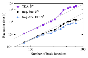
Figure 1: Timings of the sum-over-states (“TDA”), frequency-free (“freq.-free”), and density-fitted frequency-free (“freq.-free, DF”) implementations of the BSE for calculating the first excitation of a series of alkenes C_2nH_2n+2 in the aug-cc-pVDZ basis set Dunning (1989); Kendall, Dunning, and Harrison (1992); Woon and Dunning (1993), up to C₁₂H₁₄, with about 400 basis functions. For the sum-over-states implementation, we timed the diagonalization of the TDA matrix, which dominates the cost of GW and BSE calculations; for the frequency-free implementations, we timed all 8-16 matrix-vector multiplications required for convergence of the Davidson algorithm for the BSE step. Calculations were performed on a single core of an Intel Xeon Gold 6126 2.6 GHz (Skylake) central processing unit (CPU), and density-fitted calculations used the aug-cc-pVDZ-RI auxiliary basis set.

Eigenvalues and eigenvectors of $\bm{\mathcal{H}}$ can be obtained by iterative diagonalization using, e.g., the Davidson algorithm. Writing the solution vector as $\bm{R}=[r_{i}^{a},r_{ij}^{ab},\bar{r}_{ij}^{ab}]$, matrix-vector multiplication is given by $\bm{\mathcal{H}}\bm{R}=\bm{\sigma}$, with

$$\begin{split}\sigma_{i}^{a}&=(E_{a}-E_{i})r_{i}^{a}+\sum_{jb}\left[\kappa(ia|jb)-(ij|ab)\right]r_{j}^{b}\\ &\hskip 10.00002pt-\sqrt{2}\sum_{dkc}(kc|ad)r_{ik}^{dc}-\sqrt{2}\sum_{lkc}(il|ck)\bar{r}_{lk}^{ac}\end{split}$$ (10a)

$$\begin{split}\sigma_{lk}^{dc}&=(E_{d}-E_{l}+\varepsilon_{c}-\varepsilon_{k})r_{lk}^{dc}\\ &\hskip 10.00002pt+\sqrt{2}\sum_{i}(il|ck)r_{i}^{d}+2\sum_{ia}(kc|ia)r_{li}^{da}\end{split}$$ (10b)

$$\begin{split}\bar{\sigma}_{lk}^{dc}&=(E_{d}-E_{l}+\varepsilon_{c}-\varepsilon_{k})\bar{r}_{lk}^{dc}\\ &\hskip 10.00002pt+\sqrt{2}\sum_{a}(kc|ad)r_{l}^{a}+2\sum_{ia}(kc|ia)\bar{r}_{li}^{da}.\end{split}$$ (10c)

Eigenvalues found in this way naturally include dynamical screening and are exactly the same as those from the conventional dynamically screened BSE (within the TDA). As written, the cost of the above matrix-vector products is $O(O^{3}V^{3})$, where $O$ and $V$ are the number of occupied and virtual orbitals in the single-particle basis, or $O(N^{6})$ generically. While the prefactor is significantly smaller (see below), this reformulation exhibits the same asymptotic scaling as full diagonalization of the RPA matrix and explicit evaluation of the dynamically screened Coulomb interaction (LABEL:eq:Kd). However, the absence of exchange-type integrals in the direct RPA enables a scaling reduction through the use of density fitting with $N_{\mathrm{aux}}$ auxiliary basis functions, $(pq|rs)\approx\sum_{P}L_{pq}^{P}L_{rs}^{P}$. This leads to a reformulation of the worst scaling terms, e.g.

$$\sigma_{lk}^{dc}=2\sum_{iaP}L_{kc}^{P}L_{ia}^{P}r_{li}^{da}+\ldots$$ (11)

which now has two $O(N_{\mathrm{aux}}O^{2}V^{2})$ steps or $O(N^{5})$ overall.

In Fig. 1, we show the execution time of dynamical BSE calculations for a series of alkenes of increasing length. As long as only a few BSE eigenvectors are required, the reformulation to an iterative eigenvalue problem is seen to reduce the $N^{6}$ prefactor by about two orders of magnitude. The use of density fitted integrals changes the scaling to $O(N^{5})$. For a system with hundreds of basis functions, selected BSE eigenvalues can be found in a few minutes on a single core. Further timing details are given in the caption of Fig. 1. We recall that an exact BSE calculation (within a basis) requires, as input, all GW quasiparticle eigenvalues. As long as an $O(N^{4})$ GW method is used to find the $O(N)$ GW eigenvalues, then this initial calculation also has $O(N^{5})$ scaling, and so the asymptotic scaling of the full GW/BSE calculation is $O(N^{5})$.

In most GW/BSE calculations, RPA screening is used without the TDA (even though the TDA is commonly made in a subsequent BSE calculation), but our frequency-free implementation is simplest with the TDA. Therefore, we assessed the accuracy of this approximation by comparing to the “theoretical best estimate” excitation energies of the molecules in the Thiel set Schreiber et al. (2008). In Fig. 2, we show that when PBE and PBE0 references are used, the excitation energies obtained with TDA screening exhibit errors that are generally larger than or similar to those obtained with RPA screening (slightly worse for singlets and slightly better for triplets). However, a HF reference provides smaller errors than these two DFT references. Perhaps surprisingly, we find that the most accurate results are those obtained when a HF reference is combined with TDA screening, achieving an accuracy of about 0.2-0.3 eV and empirically justifying our use of TDA screening. This conclusion, which is the same as we previously found for ionization potentials of molecules within the GW approximation, Bintrim and Berkelbach (2021) may change when GW/BSE is applied to solids, especially metals and small gap semiconductors that are highly polarizable.

One might ask whether the GW/BSE@HF results with TDA screening are the most accurate because (a) TDA screening is best for both GW and the BSE or (b) TDA screening is best for GW but not the BSE. To test this, we combined TDA-GW eigenvalues with an RPA-screened Coulomb interaction in the BSE. The accuracy of the singlet excitations was not significantly different, and triplets were slightly less accurate, further justifying our use of TDA screening for both steps of a GW/BSE@HF calculation.

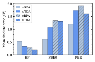
Figure 2: Mean absolute errors in singlet (s) and triplet (t) excitation energies calculated using the dynamical GW/BSE with RPA Loos and Blase (2020) and TDA screening, starting from three mean-field references. Statistics were collected for all excitations with less than 50% double excitation character Harbach, Wormit, and Dreuw (2014) for the 25 smallest molecules in the Thiel set Schreiber et al. (2008) in the def2-TZVP basis Weigend and Ahlrichs (2005). Error is calculated with respect to the first Thiel set theoretical best estimates. Silva-Junior et al. (2010)

As mentioned previously, the BSE with static screening (or with perturbative corrections to account for dynamical screening Loos and Blase (2020)) cannot access excited states of primarily double excitation character. Therefore, to the best of our knowledge, the performance of GW/BSE on double excitations has not been assessed. This is distinct from the GW approximation, where satellite structures in the spectral function due to hole-plasmon coupling, i.e., double excitations and higher, have been studied extensively Hedin and Lundqvist (1970); Guzzo et al. (2011); Zhou et al. (2015). Using our frequency-free formulation of the BSE, we are well-positioned to evaluate its performance for double excitations. As an example, we have studied the $2^{1}$A_g excitation of butadiene, hexatriene, and octatetraene, which is known to have substantial double excitation character Cave et al. (2004); Starcke et al. (2006); Romaniello et al. (2009); Angeli and Pastore (2011); Harbach, Wormit, and Dreuw (2014); Loos et al. (2019); Manna, Chaudhuri, and Chattopadhyay (2020). Table 1 provides our GW/BSE@HF excitation energies and the percentage contribution of doubles excitations (%$R_{2}$) to the eigenvector. We also list theoretical best estimates (“TBE-1”) Silva-Junior et al. (2010) and literature values from strict and extended ADC(2), EOM-CCSD, and ADC(3) methods.

Overall, we see that GW/BSE@HF provides a poor description of double excitations, overestimating their energy by about 1.5–2 eV and significantly underestimating their double excitation character. This behavior is similar to that exhibited by strict ADC(2) and EOM-CCSD. We tentatively conclude that the dynamical BSE provides a qualitative but not quantitative description of doubly excited states, but more thorough testing is required.

Table 1: Excitation energies (eV) and percentage doubles character (“%$R_{2}$”) for the $2^{1}$A${}_{\text{g}}$ excitation in three alkenes (C_2nH_2n+2) calculated with the def2-TZVP Weigend and Ahlrichs (2005) basis set. Theoretical best estimate (TBE-1) results are from Ref. Silva-Junior et al., 2010 and all ADC and EOM-CCSD results are from Ref. Harbach, Wormit, and Dreuw, 2014.

	butadiene		hexatriene		octatetraene
	$E$	%$R_{2}$	$E$	%$R_{2}$	$E$	%$R_{2}$
TBE-1	6.55	-	5.09	-	4.47	-
BSE	8.02	8	7.09	9	6.33	10
ADC(2)-s	7.68	10	6.72	12	5.93	13
ADC(2)-x	5.12	59	4.02	66	3.30	70
ADC(3)	5.77	68	4.52	77	3.73	80
EOM-CCSD	7.42	24	6.61	24	5.99	21

Before concluding, we note that our frequency-independent matrix $\bm{\mathcal{H}}$ that is represented in a basis of single and double excitations is superficially similar to the one appearing in configuration interaction or the ADC, but it is asymmetric, has two sets of double excitations, and requires correlated GW eigenvalues as input. With some approximations, it can be brought to a more familiar form,

$$\bm{\tilde{\mathcal{H}}}=\left(\begin{array}[]{ccc}\mathbf{\tilde{A}}&\mathbf{V}^{\text{e}}-\mathbf{V}^{\text{h}}\\ (\mathbf{V}^{\text{e}}-\mathbf{V}^{\text{h}})^{\dagger}&\mathbf{\tilde{D}}\end{array}\right)$$ (12)

where

$$\tilde{A}_{ia,jb} =(\varepsilon_{a}-\varepsilon_{i})\delta_{ij}\delta_{ab}+\kappa(ia|jb)-(ij|ab)$$ (13a)

$$\mathbf{\tilde{D}} =[-\bm{\varepsilon}_{\text{occ}}]\oplus\bm{\varepsilon}_{\text{vir}}\oplus\mathbf{S}.$$ (13b)

Note that all orbital energies are now mean-field energies; therefore this formulation has the advantage of not requiring an initial GW calculation. Instead, this formulation has a natural self-energy-like correction,

$$\mathbf{\tilde{\Sigma}}(\omega) =\mathbf{V}^{\text{e}}(\omega\mathbf{I}-\mathbf{\tilde{D}})^{-1}(\mathbf{V}^{\text{e}})^{\dagger}+\mathbf{V}^{\text{h}}(\omega\mathbf{I}-\mathbf{\tilde{D}})^{-1}(\mathbf{V}^{\text{h}})^{\dagger}$$ (14a)

$$\begin{split}\tilde{\Sigma}_{ia,jb}(\omega)&=\delta_{ij}\sum_{km}\frac{(ik|\rho_{m})(jk|\rho_{m})}{\omega-(\epsilon_{a}-\epsilon_{k}+\Omega_{m})}\\ &\hskip 10.00002pt+\delta_{ab}\sum_{cm}\frac{(ac|\rho_{m})(bc|\rho_{m})}{\omega-(\epsilon_{c}-\epsilon_{i}+\Omega_{m})},\end{split}$$ (14b)

with a frequency argument to be evaluated at the neutral BSE excitation energies.

Despite its attractive features and essential GW/BSE physics, our testing (not shown) indicates that the matrix (12) has eigenvalues that are about 2–3 eV below our exact dynamical BSE results. We attribute this discrepancy to the fact that the self-energy-like correction (14) has only forward time-ordered diagrams, i.e., the particle propagator is only renormalized by two-particle+one-hole configurations and not by two-hole+one-particle configurations and vice versa for the hole propagator. Making this approximation in a GW calculation was observed to severely affect the GW eigenvalues, which yielded similarly poor neutral excitation energies when used in a subsequent BSE calculation.

To summarize, we have shown that the conventionally frequency-dependent dynamical BSE can be exactly reformulated into a frequency-independent eigenvalue problem in an expanded space of single and double excitations, enabling a reduced cost implementation and a study of doubly excited states. We anticipate that this reformulation will enable future methodological developments to account for, for example, orbital optimization or multiconfigurational reference wavefunctions. It would be interesting to explore extensions of the cumulant approach, which provides an improved description of satellite peaks in the one-particle spectral function Aryasetiawan, Hedin, and Karlsson (1996); Guzzo et al. (2011), to two-particle response functions Zhou et al. (2015); Kas, Rehr, and Curtis (2016). Similarly, while our current work has studied double excitations in gapped molecules, it would be interesting to perform analogous studies in bulk materials to study biexcitons, exciton-plasmon interactions, or plasmon lifetimes Lewis and Berkelbach (2019) within the GW/BSE framework.

Data availability statement

The data that support the findings of this study are available from the corresponding author upon reasonable request.

References

- Hedin (1965) L. Hedin, Phys. Rev. 139, A796 (1965).
- Strinati (1988) G. Strinati, Riv. del Nuovo Cim. 11, 1 (1988).
- Hanke and Sham (1980) W. Hanke and L. J. Sham, Phys. Rev. B 21, 4656 (1980).
- Strinati (1984) G. Strinati, Phys. Rev. B 29, 5718 (1984).
- Albrecht et al. (1998) S. Albrecht, L. Reining, R. D. Sole, and G. Onida, Phys. Stat. Sol. A 170, 189 (1998).
- Rohlfing and Louie (2000) M. Rohlfing and S. G. Louie, Phys. Rev. B 62, 4927 (2000).
- Tiago and Chelikowsky (2005) M. L. Tiago and J. R. Chelikowsky, Solid State Commun. 136, 333 (2005).
- Faber et al. (2014) C. Faber, P. Boulanger, C. Attaccalite, I. Duchemin, and X. Blase, Philos. Trans. R. Soc. A: Math. Phys. Eng. Sci. 372, 20130271 (2014).
- Körbel et al. (2014) S. Körbel, P. Boulanger, I. Duchemin, X. Blase, M. A. L. Marques, and S. Botti, J. Chem. Theory Comput. 10, 3934 (2014).
- Bruneval, Hamed, and Neaton (2015) F. Bruneval, S. M. Hamed, and J. B. Neaton, J. Chem. Phys. 142, 244101 (2015).
- Jacquemin, Duchemin, and Blase (2015) D. Jacquemin, I. Duchemin, and X. Blase, J. Chem. Theory Comput. 11, 3290 (2015).
- Rangel et al. (2017) T. Rangel, S. M. Hamed, F. Bruneval, and J. B. Neaton, J. Chem. Phys. 146, 194108 (2017).
- Blase et al. (2020) X. Blase, I. Duchemin, D. Jacquemin, and P.-F. Loos, J. Phys. Chem. Lett. 11, 7371 (2020).
- Jacquemin et al. (2016) D. Jacquemin, I. Duchemin, A. Blondel, and X. Blase, J. Chem. Theory Comput. 12, 3969 (2016).
- Jacquemin, Duchemin, and Blase (2017) D. Jacquemin, I. Duchemin, and X. Blase, J. Phys. Chem. Lett. 8, 1524 (2017).
- Blase, Duchemin, and Jacquemin (2018) X. Blase, I. Duchemin, and D. Jacquemin, Chem. Soc. Rev. 47, 1022 (2018).
- Gui, Holzer, and Klopper (2018) X. Gui, C. Holzer, and W. Klopper, J. Chem. Theory Comput. 14, 2127 (2018).
- Rocca, Lu, and Galli (2010) D. Rocca, D. Lu, and G. Galli, J. Chem. Phys. 133, 164109 (2010).
- Krause and Klopper (2017) K. Krause and W. Klopper, J. Comput. Chem. 38, 383 (2017).
- Bruneval et al. (2016) F. Bruneval, T. Rangel, S. M. Hamed, M. Shao, C. Yang, and J. B. Neaton, Comput. Phys. Commun. 208, 149 (2016).
- Liu et al. (2020) C. Liu, J. Kloppenburg, Y. Yao, X. Ren, H. Appel, Y. Kanai, and V. Blum, J. Chem. Phys. 152, 044105 (2020).
- Ma, Rohlfing, and Molteni (2009) Y. Ma, M. Rohlfing, and C. Molteni, J. Chem. Theory Comput. 6, 257 (2009).
- Loos and Blase (2020) P.-F. Loos and X. Blase, J. Chem. Phys. 153, 114120 (2020).
- Romaniello et al. (2009) P. Romaniello, D. Sangalli, J. A. Berger, F. Sottile, L. G. Molinari, L. Reining, and G. Onida, J. Chem. Phys. 130, 044108 (2009).
- Elliott et al. (2011) P. Elliott, S. Goldson, C. Canahui, and N. T. Maitra, Chem. Phys. 391, 110 (2011).
- Authier and Loos (2020) J. Authier and P.-F. Loos, J. Chem. Phys. 153, 184105 (2020).
- Bintrim and Berkelbach (2021) S. J. Bintrim and T. C. Berkelbach, J. Chem. Phys. 154, 041101 (2021).
- van Setten et al. (2015) M. J. van Setten, F. Caruso, S. Sharifzadeh, X. Ren, M. Scheffler, F. Liu, J. Lischner, L. Lin, J. R. Deslippe, S. G. Louie, C. Yang, F. Weigend, J. B. Neaton, F. Evers, and P. Rinke, J. Chem. Theory Comput. 11, 5665 (2015).
- Dunning (1989) T. H. Dunning, J. Chem. Phys. 90, 1007 (1989).
- Kendall, Dunning, and Harrison (1992) R. A. Kendall, T. H. Dunning, and R. J. Harrison, J. Chem. Phys. 96, 6796 (1992).
- Woon and Dunning (1993) D. E. Woon and T. H. Dunning, J. Chem. Phys. 98, 1358 (1993).
- Schreiber et al. (2008) M. Schreiber, M. R. Silva-Junior, S. P. A. Sauer, and W. Thiel, J. Chem. Phys. 128, 134110 (2008).
- Harbach, Wormit, and Dreuw (2014) P. H. P. Harbach, M. Wormit, and A. Dreuw, J. Chem. Phys. 141, 064113 (2014).
- Weigend and Ahlrichs (2005) F. Weigend and R. Ahlrichs, Phys. Chem. Chem. Phys. 7, 3297 (2005).
- Silva-Junior et al. (2010) M. R. Silva-Junior, M. Schreiber, S. P. A. Sauer, and W. Thiel, J. Chem. Phys. 133, 174318 (2010).
- Hedin and Lundqvist (1970) L. Hedin and S. Lundqvist, Solid State Phys. 23, 1 (1970).
- Guzzo et al. (2011) M. Guzzo, G. Lani, F. Sottile, P. Romaniello, M. Gatti, J. J. Kas, J. J. Rehr, M. G. Silly, F. Sirotti, and L. Reining, Phys. Rev. Lett. 107, 166401 (2011).
- Zhou et al. (2015) J. S. Zhou, J. J. Kas, L. Sponza, I. Reshetnyak, M. Guzzo, C. Giorgetti, M. Gatti, F. Sottile, J. J. Rehr, and L. Reining, J. Chem. Phys. 143, 184109 (2015).
- Cave et al. (2004) R. J. Cave, F. Zhang, N. T. Maitra, and K. Burke, Chem. Phys. Lett. 389, 39 (2004).
- Starcke et al. (2006) J. H. Starcke, M. Wormit, J. Schirmer, and A. Dreuw, Chem. Phys. 329, 39 (2006).
- Angeli and Pastore (2011) C. Angeli and M. Pastore, J. Chem. Phys. 134, 184302 (2011).
- Loos et al. (2019) P.-F. Loos, M. Boggio-Pasqua, A. Scemama, M. Caffarel, and D. Jacquemin, J. Chem. Theory Comput. 15, 1939 (2019).
- Manna, Chaudhuri, and Chattopadhyay (2020) S. Manna, R. K. Chaudhuri, and S. Chattopadhyay, J. Chem. Phys. 152, 244105 (2020).
- Aryasetiawan, Hedin, and Karlsson (1996) F. Aryasetiawan, L. Hedin, and K. Karlsson, Phys. Rev. Lett. 77, 2268 (1996).
- Kas, Rehr, and Curtis (2016) J. J. Kas, J. J. Rehr, and J. B. Curtis, Phys. Rev. B 94, 035156 (2016).
- Lewis and Berkelbach (2019) A. M. Lewis and T. C. Berkelbach, Phys. Rev. Lett. 122, 226402 (2019).