FOCUS: Familiar Objects in Common and Uncommon Settings

Abstract

Standard training datasets for deep learning often do not contain objects in uncommon and rare settings (e.g., “a plane on water”, “a car in snowy weather”). This can cause models trained on these datasets to incorrectly predict objects that are typical for the context in the image, rather than identifying the objects that are actually present. In this paper, we introduce FOCUS (Familiar Objects in Common and Uncommon Settings), a dataset for stress-testing the generalization power of deep image classifiers. By leveraging the power of modern search engines, we deliberately gather data containing objects in common and uncommon settings; in a wide range of locations, weather conditions, and time of day. We present a detailed analysis of the performance of various popular image classifiers on our dataset and demonstrate a clear drop in accuracy when classifying images in uncommon settings. We also show that finetuning a model on our dataset drastically improves its ability to focus on the object of interest leading to better generalization. Lastly, we leverage FOCUS to machine annotate additional visual attributes for the entirety of ImageNet. We believe that our dataset will aid researchers in understanding the inability of deep models to generalize well to uncommon settings and drive future work on improving their distributional robustness.

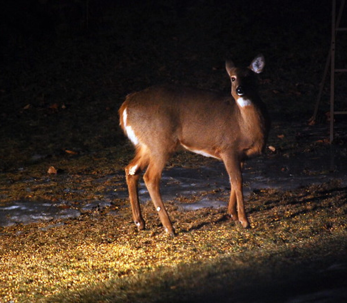
(a) deer at night

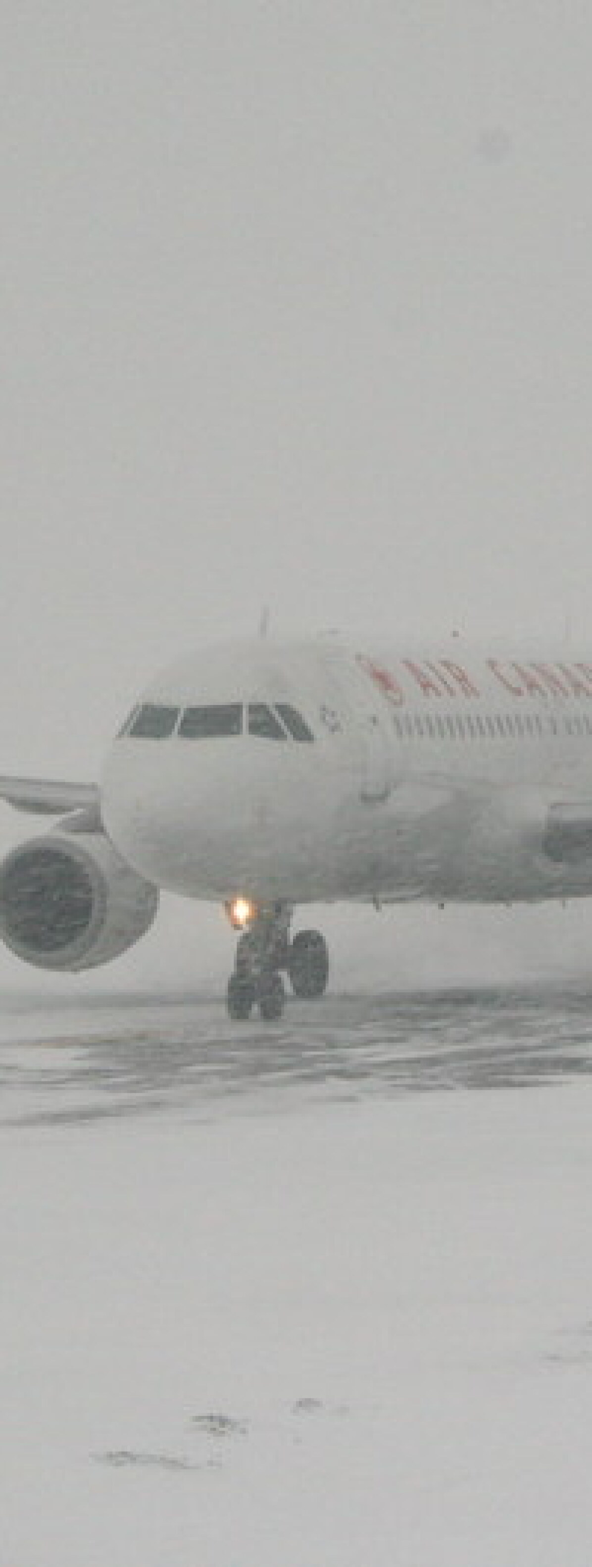
(b) plane in snowy weather

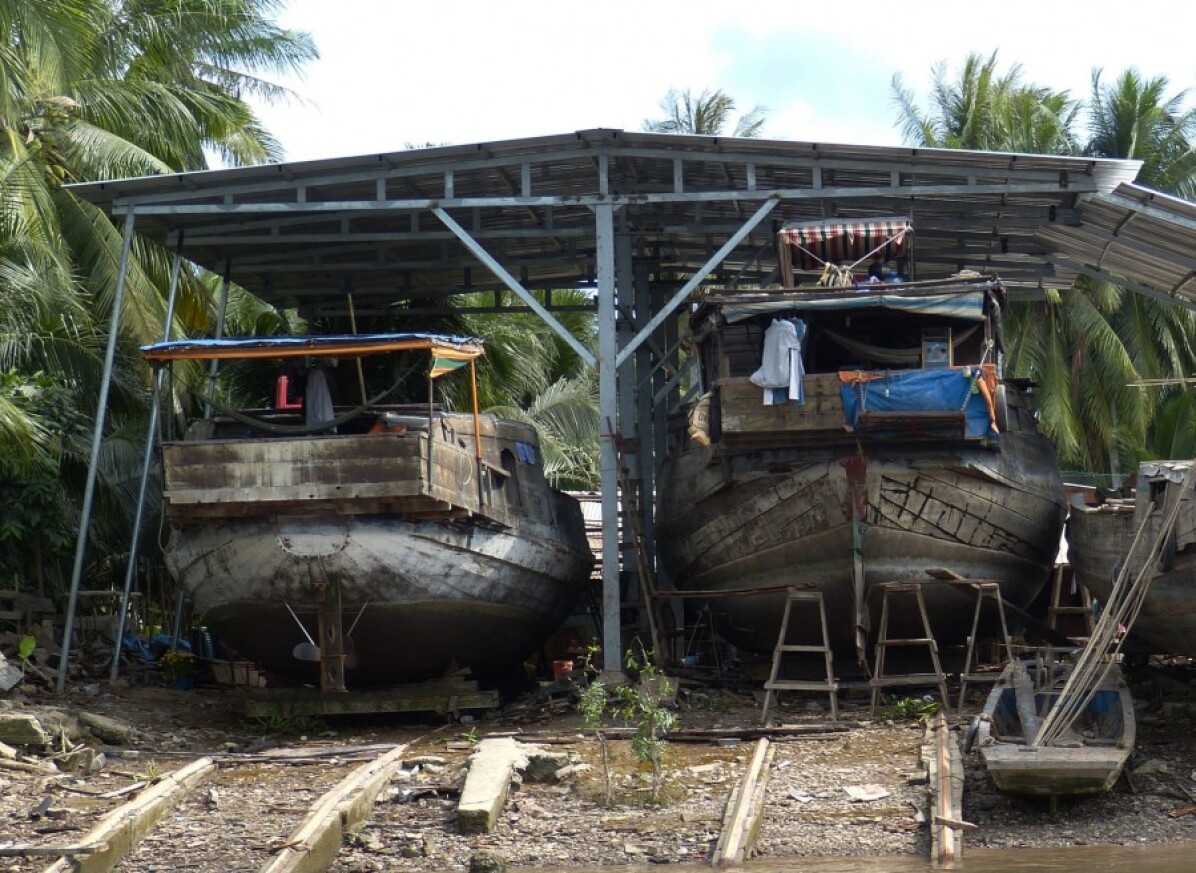
(c) ship indoors

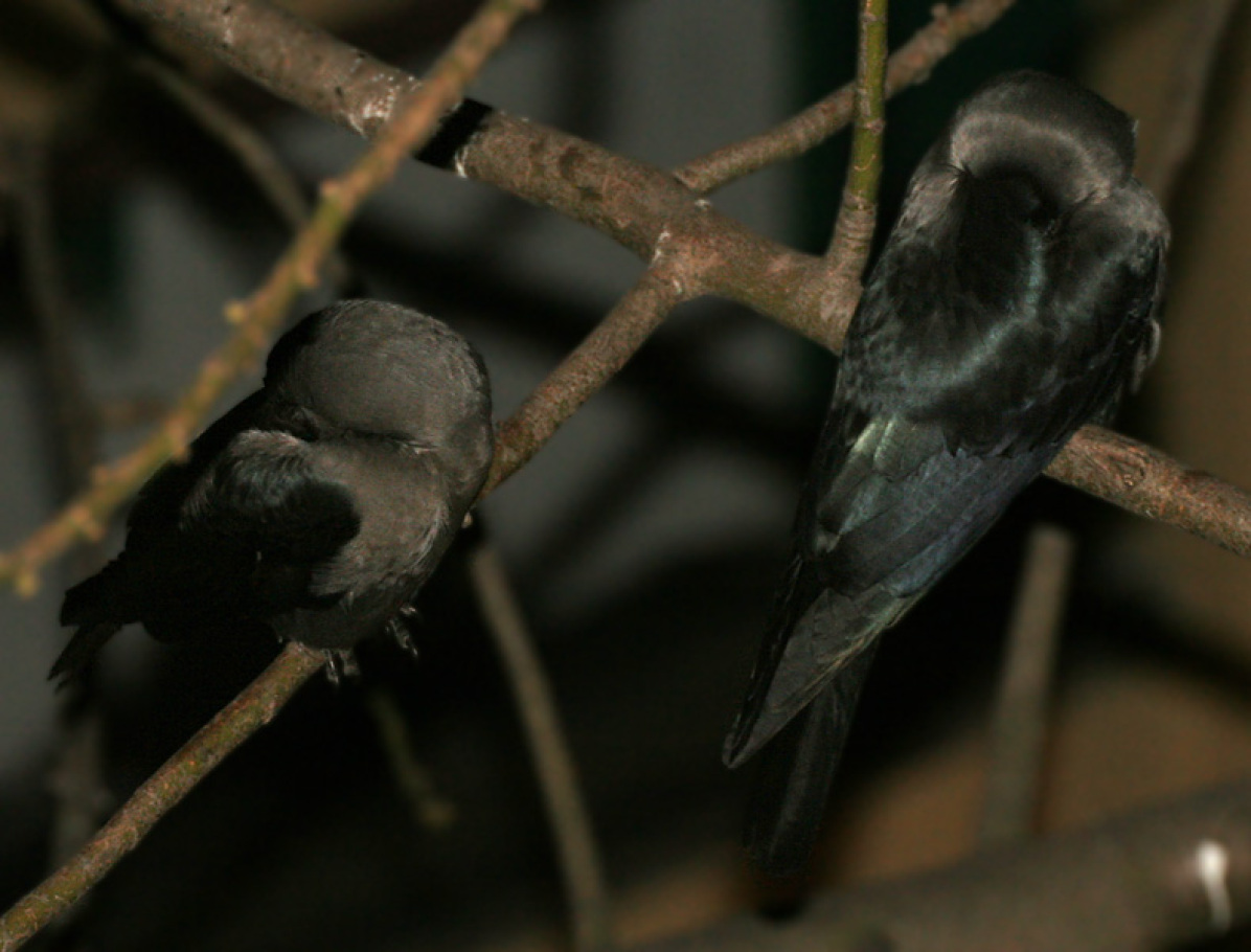
(d) bird at night

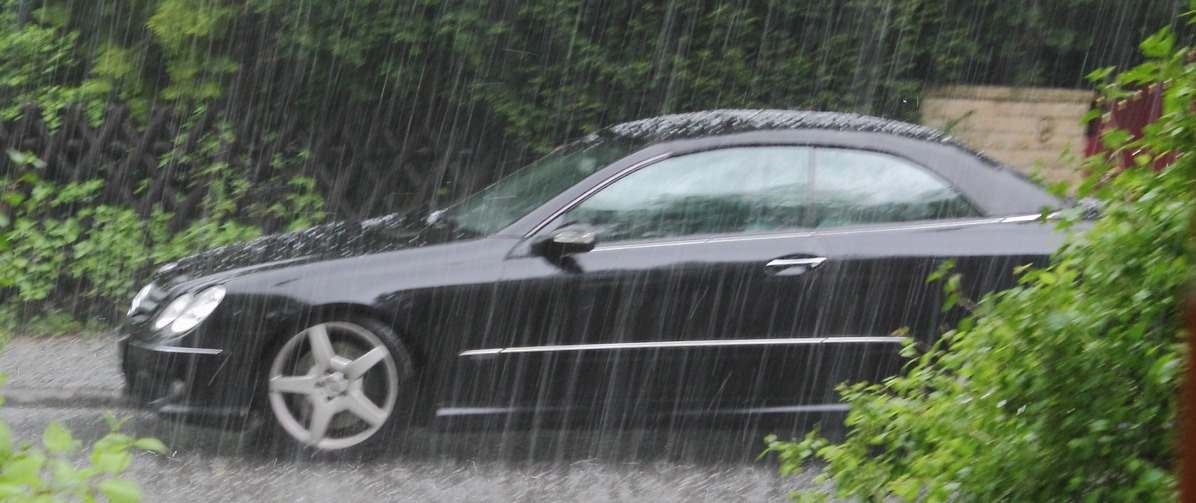
(e) car in rain

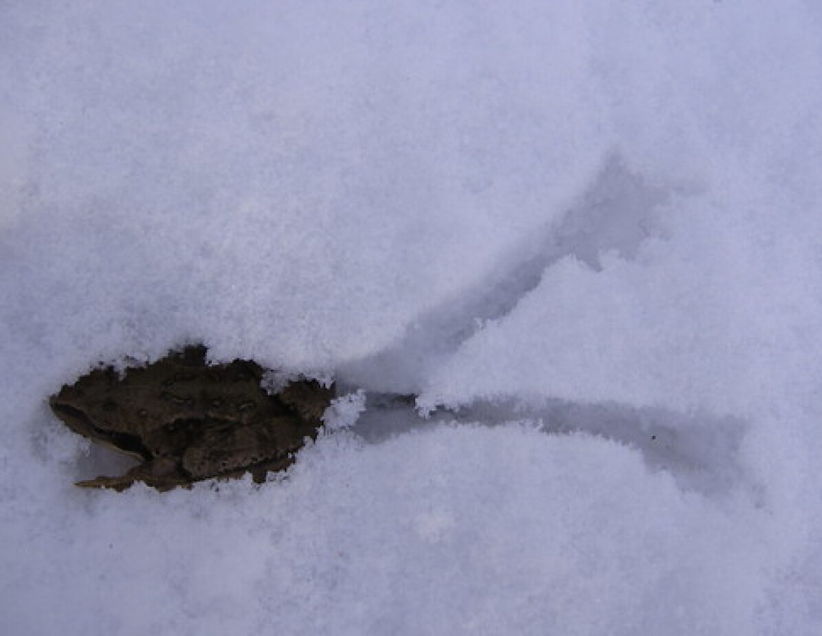
(f) frog in snow

Figure 1: Some uncommon images in the FOCUS dataset. The images in the first column depict uncommon time of day, those in the second column depict uncommon weather, and the ones in the third column depict uncommon locations.

1 Introduction

Since the remarkable success of AlexNet (Krizhevsky et al., 2012) in the ImageNet Large Scale Visual Recognition Challenge (ILSVRC) (Russakovsky et al., 2015), deep learning models have been used in a variety of applications ranging from robotics and self-driving cars to stock trading and computational biology. Undoubtedly, large scale datasets such as ImageNet (Deng et al., 2009) deserve much of the credit for the success of deep learning. These datasets typically consist of natural images of objects in some environment. For our purposes, the environment in an image includes all the contextual information surrounding the object in the image. Evidently, objects do not occur independently of their environments. In other words, objects are more likely to be found in some environments than in others (we call these common settings). For example, ships are often on water; cars are usually on streets; birds are usually on trees, etc. Search engines are more likely to return images with objects in their common settings when queried for an object alone, i.e., without any additional qualifiers (e.g., just “deer” or “frog”). As a result, objects in uncommon settings are often missing in many of the popular datasets in use today. Therefore, a classifier’s performance on these datasets is not indicative of how well it does in novel environments.

To address this issue, we introduce a new dataset containing images both in common and uncommon settings called FOCUS (Familiar Objects in Common and Uncommon Settings). Our key idea is that modern search engines often return many relevant results even for qualified queries of objects in uncommon settings. For example, searching “bird indoors” still returns a few relevant images even though this is an uncommon setting. Building on this idea, we collect images of objects in various common and uncommon environments explicitly. FOCUS has around 21K images of ten objects along with annotations for different aspects of the environment in the images including a wide range of locations, weather conditions, and time of day. Depending on the class, we further annotate these environmental settings as common or uncommon.

Using FOCUS, we assess the performance of some popular deep learning models with high accuracy on ImageNet, on uncommon settings. We observe that all of these popular models show significant drop in accuracy when tested on objects in uncommon settings. Next, we finetune these models on FOCUS and show clear evidence for substantial improvement in generalization. We also use FOCUS to train classifiers that can detect various visual attributes we consider in FOCUS and use these classifiers to add additional annotations to ImageNet. To the best of our knowledge, FOCUS is the first large-scale dataset of natural images with explicit environmental annotations such as locations, weather conditions, and time of day for both common and uncommon settings. We believe richly annotated datasets such as FOCUS can pave the way to develop models that not only have high accuracy in common settings but are reliable in rare and uncommon settings as well. Our dataset and code for evaluating models on FOCUS are available at https://github.com/priyathamkat/focus.

2 Related Work

Deep neural networks are well known to rely on spurious features or “shortcuts” for image classification and object detection (Geirhos et al., 2020). Beery et al. (2018) demonstrate this phenomenon in the case of detection and classification of animals in uncommon locations; cows are improperly detected or incorrectly classified in beaches. Sagawa* et al. (2020) show a similar issue in regard to classification of waterbirds and the color of human hair in CelebA (Liu et al., 2015). Rosenfeld et al. (2018) observe that object detectors may not always detect objects artificially placed into an image. Further, these objects can have a non-local impact, causing the detector to not detect other objects in the image.

In light of the above, test accuracy on datasets like CIFAR (Krizhevsky et al., 2014), ImageNet (Deng et al., 2009), etc., though crucial, is insufficient to measure the efficacy of deep neural networks. Many datasets have been proposed in the literature for testing the out-of-distribution effectiveness of classification models. Hendrycks et al. (2021a) propose three datasets, namely, ImageNet-Renditions, DeepFashion Remixed, StreetView StoreFronts that are designed to test the generalization ability of classifiers to unseen rendition styles, camera view points, and geography, respectively. Barbu et al. (2019) propose ObjectNet, a dataset that provides a far richer variation in the rotation, viewpoint and backgrounds of many object classes in ImageNet. They observe that models trained on ImageNet are 40-45% less accurate on ObjectNet. Realistic corruptions such as blur, noise, etc., can occur in the real world, for instance, due to camera shake, low light, etc. Thus, training on high-quality clean images may cause classifiers to perform poorly on corrupted images. Hendrycks & Dietterich (2019) propose ImageNet-C, a dataset of 15 types of artifically corrupted images to systematically study robustness of deep learning models against (synthetic) corruptions. Hendrycks et al. (2021a) propose Real Blurry Images, a dataset of 1000 real world blurry images. ImageNet-A (Hendrycks et al., 2021b) is a dataset of natural, adversarial images which yield drastically low performance on classifiers trained on ImageNet.

In parallel to OOD datasets, many works have been proposed to explicitly find the spurious dependencies on context and/or circumvent them. Singla et al. (2021) propose a method for identifying the visual attributes that cause classification failures using the features of an adversarially robust model. Xiao et al. (2020) propose the Backgrounds Challenge to evaluate how robust models are to (synthetic) changes in backgrounds. Sauer & Geiger (2021) propose a generative framework which allows choosing the color, texture and background of a generated image independently. Using this, they generate counterfactual images and show that training on these images improves out-of-distribution robustness. BDD100K(Yu et al., 2020) is a large scale video dataset for driving that covers a wide range of locations, environments and weather conditions. Wong et al. (2021) show that training sparse linear models with deep features as inputs results in improved debuggability of neural networks. In a similar vein, 3DB (Leclerc et al., 2021) uses photorealistic simulations to test and debug computer vision models. Beery et al. (2018) introduce a dataset of camera trap images. Since, the traps are fixed, the backgrounds in these images are also more or less fixed and hence this dataset provides an ideal testing ground for classification/detection in uncommon contexts.

A large body of influential work proposes models that explicitly use context to improve image classification or object detection performance. Galleguillos et al. (2008) use a conditional random field to incorporate spatial and semantic context. Mottaghi et al. (2014) propose a deformable parts based model that uses both local and global context to improve object detection at various scales. Bell et al. (2016) present a novel architecture called the Inside-Outside Net which uses skip pooling to extract context inside the region of interest while the information from outside the ROI is extracted through spatial recurrent neural networks. Choi et al. (2012) build an explicit support context model to capture inter-object physical relationships and use it to detect out-of-context objects. Lastly, Divvala et al. (2009) is an extensive survey on the role of various types of context in object detection.

Table 1: A frequency breakdown of the various categories and attributes in the FOCUS dataset. Uncommon settings are highlighted in orange.

		Truck	Car	Plane	Ship	Cat	Dog	Horse	Deer	Frog	Bird
Time of Day	Day	1036	2232	1498	1573	1809	2415	2989	1622	931	2298
	Night	50	241	128	159	72	56	60	51	180	45
	None	29	212	109	29	941	503	66	34	323	124
Weather	Cloudy	139	301	259	324	50	151	186	95	17	171
	Foggy	27	103	56	109	7	46	105	78	1	43
	Partly Cloudy	145	310	305	309	111	170	284	175	44	151
	Raining	10	92	19	7	11	7	14	2	3	17
	Snowing	9	39	4	3	23	39	36	44	0	32
	Sunny	538	956	694	687	639	1083	957	742	423	1184
	None	247	884	398	322	1981	1478	533	571	946	869
Locations	Forest	172	378	178	79	123	247	586	916	142	400
	Grass	326	651	391	105	517	804	1142	1255	274	541
	Indoors	31	259	125	5	1344	790	93	10	39	40
	Rocks	43	115	55	71	137	109	92	95	239	183
	Sand	295	526	239	187	143	414	662	214	152	296
	Street	708	1635	389	103	405	372	417	103	29	130
	Snow	88	255	110	140	127	298	206	290	7	176
	Water	46	211	296	1606	93	403	296	122	355	581
	None	56	96	526	51	372	279	146	49	446	699

3 FOCUS: A Dataset with Common and Uncommon Settings

3.1 Building FOCUS

We use the time of day, weather and the locations depicted in an image to characterize environment in it. Modern search engines are capable of returning relevant results even for uncommon qualified queries of objects (e.g., “frog indoors”). We leverage this to collect images of objects in various common and uncommon environments explicitly. Concretely, we query the Microsoft Bing Image Search API with statements of the form <object>  <preposition>  <attribute>  (e.g., “ship on grass”). This ensures that we collect a great variety of uncommon images. We also use synonyms of the object categories and the attributes to increase the number of samples we collect. Note that we only query for images which have a license that permits sharing allowing us to release the FOCUS dataset for the research community.

We collect a total of around 37K images using the above procedure. But the search results are not always accurate; a significant fraction of them do not have the relevant object or if they do, the object is not in the environment mentioned in the search query. In addition, because we query images based on only one attribute, we do not have any information about the other attributes in the images. For instance, we do not know the time of day or the locations in a search result for “car in rain”.

We conduct an Amazon Mechanical Turk study both to improve the accuracy of annotations inferred from the search queries and to collect missing annotations. Images are shown to workers in a series of Human Intelligence Tasks (HITs), and they are asked to annotate the image with the appropriate choice for the different attributes. See the appendix B for more details about the design of our HITs.

3.2 The Data in FOCUS

The FOCUS dataset is a collection of around 21K images, each annotated with the time of day, the weather condition and the locations in the image. Concretely, our dataset is as follows:

$$\{(\mathbf{x}_{i},y_{i},t_{i},w_{i},l_{i})\}_{i=1}^{n}$$

where

$$\mathbf{x}_{i}\text{ is the image}$$

$$y_{i}\text{ is the object label}\in\{\textit{truck, car, plane, ship, cat, dog,}$$

$$\qquad\qquad\qquad\qquad\quad\,\,\,\,\textit{horse, deer, frog, bird}\}$$

$$t_{i}\text{ is the time of day}\in\{\textit{day, night, none}\}$$

$$w_{i}\text{ is the weather}\in\{\textit{cloudy, foggy, partly cloudy, raining,}$$

$$\qquad\qquad\qquad\qquad\,\,\,\textit{snowing, sunny, none}\}$$

$$l_{i}\text{ are the locations}\subset\{\textit{forest, grass, indoors, rocks, sand,}$$

$$\qquad\qquad\qquad\qquad\quad\textit{street, snow, water, none}\}$$

The rationale behind our choices for different attributes is as follows:

1. Object Label: We choose to work with the same 10 object classes in CIFAR-10 (Krizhevsky et al., 2014). These classes cover 226 (including various birds, animals and vehicles) of the 1000 classes in ImageNet.

2. Time of day: Most images in standard datasets are captured during the day, when the objects are well lit. In contrast, nighttime images often lack a lot of details and are corrupted by high levels of noise.

3. Weather: Our choices of weather are fairly comprehensive and include the raining, snowing and foggy conditions which often produce natural corruptions in images.

4. Locations: We choose a wide range of locations with a healthy mix between common and uncommon (object, location) pairs. Since images are often likely to include a combination of locations, we let the locations attribute of an image to be a subset of the above set instead of being exactly one element out of it.

“none” is assigned to an attribute if its ambiguous or impossible to determine from the image. In addition, “none” is also assigned to $l_{i}$ of an image if none of the considered locations is in the image. Table 1 summarizes the number of FOCUS samples for each object in various environments.

3.3 Common vs. Uncommon Settings

We consider two sources of uncommon (object, environment) pairs:

1. The pair is uncommon in the real world (e.g., “ship on grass”). On the Internet, searching for “ship” alone is extremely unlikely to return any images of a ship on grass in the top results. In other words, the rarity of a pair in the real world is reflected in the dataset.

2. The pair is uncommon due to the choice of labels and queries used to construct a particular benchmark. For example, consider the “plane” class. ImageNet has two labels corresponding to an airplane: “warplane, military plane”, “airliner”. Neither of these are planes that are usually found on water making (“plane in water”) an uncommon, if not a non-existent pair in ImageNet. Seaplanes, however, are not that uncommon in the real world.

We declare an (object, attribute) uncommon if the number of samples corresponding to that pair is low (case 1 above). Additionally, we also declare the (“plane”, “water”) pair as uncommon (case 2 above). Our final choices for uncommon settings are highlighted in orange, in table 1. Figure 1 shows some uncommon images from our dataset.

We believe that assigning “night” as uncommon Time of Day and “snowing”, “raining”, “foggy” as uncommon Weather is reasonable. However, categorizing locations into common and uncommon settings for various objects is more subjective. In order to further justify our assignments, we use Gram matrices to identify out-of-distribution samples (Sastry & Oore, 2020). We first compute the Gram matrix deviations for images in the validation set of ImageNet. Next, we identify the threshold that achieves a 95% true positive rate (TPR) for these images. Finally, we compute the same deviations for images in FOCUS and note the fraction (table 2) of images with deviations above the threshold. For each class (row), we see that the locations with higher percentages are, generally speaking, tagged as uncommon (highlighted in orange).

Table 2: Uncommon locations (highlighted in orange) in FOCUS are OOD with respect to ImageNet. Higher percentages (see text for details) indicate that the corresponding images are out-of-distribution.

	Forest	Grass	Indoors	Rocks	Sand	Street	Snow	Water
Truck	70.9	71.3	70	78.8	70.7	66.4	73.8	71.4
Car	69.4	68.7	68.1	72.6	74.5	65.2	68.9	73.1
Plane	88.2	89.4	91.5	92.6	91.1	88.6	85.8	91.9
Ship	62.7	63.5	90	62.6	62.8	56.8	63.9	61.8
Cat	78.7	78.3	73.6	71.8	78.1	71.9	77.6	75.9
Dog	28.8	29	27	30.2	32.2	26	29.4	33.1
Horse	86.9	86.8	91.7	87.9	88.7	86.1	88.6	89.2
Deer	81.1	81.2	86.7	81.5	78.8	77.7	83.6	77
Frog	76.2	74.4	75	75.6	76.1	76.7	77.5	72.9
Bird	30.6	34.7	27.5	34.4	35.5	36.8	35.5	35.6

We acknowledge that this is by no means the one true way. We facilitate other studies opting to do it in other ways by providing all annotations for the collected samples in our dataset, FOCUS.

3.4 Why FOCUS?

Consider a dataset for image classification, that is constructed by collecting samples for each object class without controlling for the environment the object is in. If the images are collected from the internet, using a search engine, then the distribution of images in the dataset reflects that of the search results. Barring any bias in the search engine, it is reasonable to expect that the images are an accurate representation of the real world. This means that for a given object, most, if not all, images will depict the object in an environment that is typical or natural for the object to be in (eg., “ship in water”). Furthermore, unless the number of samples is exceptionally large, the dataset may not contain some objects in some specific environments (eg., “plane in water”).

A deep learning model trained on such a dataset will exploit any correlation between objects and their environments in the images since context is a shortcut for identifying the object, especially when the correlation is strong. This can be troublesome when the object of interest is an atypical environment; a model that relies too much on context may fail to identify the object in the absence of context cues it has seen during training. This does not mean that all usage of context is “spurious” and undoubtedly, even humans depend on various types of context (namely semantic, spatial, pose, etc.,) (Oliva & Torralba, 2007), especially when the object is occluded or lacks discernible details. However, our argument is that humans’ use of context is nuanced; we do not look at the surroundings when we can tell what an object is simply by looking at the object alone. On the contrary, today’s deep learning models are indiscriminate in their use of context and therein lies the problem.

Lastly, we believe that FOCUS complements existing datasets such as ObjectNet (Barbu et al., 2019) by controlling for a different set of contexts, namely, illumination, weather, and location. In addition, in order to exercise a rich variation in the control variables, ObjectNet only includes objects that are easily manipulated by humans. However, our procedure for building FOCUS (Section 3.1) can be used with any object class.

4 Evaluating Deep Models on FOCUS

It is crucial to ensure that machine learning models are reliable even in rare and uncommon settings especially when they are deployed in safety-critical applications. As an example, consider a self-driving car that infers various attributes about its surroundings using deep learning models. The deployed models may be accurate in $99.99\%$ of cases that occur in common settings (e.g., pedestrian crossing on a sunny day). However, given the vast complexity of the real world, uncommon and corner cases, although rare, are still possible (e.g., a heavily snow covered car cutting in). If a model is unreliable in those uncommon settings, it could make a grave error resulting in loss of life and/or property.

In spirit of the aforementioned, we stress test the generalization power of various deep learning models to uncommon settings using the FOCUS dataset. Specifically, we are considering models that are trained using images close to the mode of the (object, environment) distribution (i.e., common images) and evaluating them on images that fall more on the tail of the (object, environment) distribution (i.e., uncommon images).

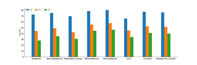
Figure 2: Top-1 classification accuracy for different models on the FOCUS dataset as a function of the partitions $P_{i}$

4.1 Experimental Setup

Model architectures.

We select some of the most popular deep learning models that have high test accuracy on ImageNet, namely ResNet50 (He et al., 2016), Wide-ResNet50-2 (Zagoruyko & Komodakis, 2016), MobileNet-v3-large (Howard et al., 2019), EfficientNet-b4 (Tan & Le, 2019), EfficientNet-b7 (Tan & Le, 2019), CLIP (Radford et al., 2021), ViT-B/16 (Dosovitskiy et al., 2021), and ResNeXt-50 (32x4d) (Xie et al., 2017). For the first three models, we use the pretrained weights provided by PyTorch (Paszke et al., 2019). We obtain the weights for both variations of EfficientNet from https://github.com/lukemelas/EfficientNet-PyTorch. We use the authors’ implementation for CLIP (from https://github.com/openai/CLIP). Following Radford et al. (2021), the text inputs to CLIP are of the form “a photo of <class>”, one for each of the 1000 classes in ImageNet. Lastly, we use timm (Wightman, 2019) for ViT-B/16 and ResNext-50 (32x4d).

Evaluation metrics.

Since the models we evaluate are pretrained on ImageNet, they output 1,000 probabilities (recall, ImageNet has 1,000 classes). On the other hand, our dataset has only 10 object categories. We resolve this apparent mismatch by first constructing a mapping (denoted by $M$) between the 1000 labels in ImageNet and those in our dataset. Concretely, a label $l_{I}$ in ImageNet is assigned to a label $l_{F}$ in our dataset if $l_{F}$ is a semantic superclass of $l_{I}$. For example, all the different dog breeds in ImageNet are mapped to the dog label in FOCUS. Decidedly, some labels in ImageNet do not have any corresponding labels in our dataset (e.g., “analog clock”, “carton” etc.). As our dataset has no images from these labels, we declare a misclassification whenever the network predicts a label that is not in the domain of $M$. We say a prediction is correct if the ImageNet label with the highest logit was assigned to the ground truth label in FOCUS. That is, for a sample $(\mathbf{x}_{i},y_{i},t_{i},w_{i},l_{i})$ from the FOCUS dataset, let $g(\mathbf{x}_{i})$ be the ImageNet label predicted by a trained network. Then, we have:

$$\text{correct prediction}\iff f(\mathbf{x}_{i})\coloneqq M(g(\mathbf{x}_{i}))=y_{i}.$$

To facilitate the evaluation of the effect of uncommon attributes, we first partition the dataset based on the number of uncommon attributes in images: $P_{i}$ is a subset of FOCUS samples with $i$ uncommon attributes for $i=0,1,2,3$. Note that $P_{0}$ denote common samples while $\bigcup_{i\geq 1}P_{i}$ denotes uncommon samples that have at least one uncommon attribute.

Table 3: Sizes of different partitions in FOCUS. $P_{i}$ is the set of images with $i$ uncommon attributes and $P^{A},\,A\subseteq\{t,w,l\}$ is the set of images where the attributes in $A$ are uncommon. Note that $P_{0}$ constitutes common images.

Total (23902)
$P_{0}$ (14144)	$P_{1}$ (5974)			$P_{2}$ (674)			$P_{3}$ (21)
	$P^{(t)}$ (641)	$P^{(w)}$ (448)	$P^{(l)}$ (4885)	$P^{(t,w)}$ (43)	$P^{(w,l)}$ (474)	$P^{(t,l)}$ (157)	$P^{(t,w,l)}$ (21)

We further subdivide $P_{i}$ into $P^{A},\,A\subseteq\{t,w,l\},\,|A|=i$ where the attributes in $A$ are uncommon (for instance, $P^{(w,l)}$ is the set of all images with two uncommon attributes: weather and location). Table 3 shows the sizes of the different partitions in our dataset.

We then evaluate the classification accuracy of different models in different partitions (referred to as $Acc(P)$). In an attempt to measure the effect of a single attribute on the accuracy of a model $f$, we define the following generalization gap with respect to an attribute $a$:

$$\begin{split}G_{a}&=\frac{|\{\mathbf{x}_{i}\in\text{C}(a)\mid f(\mathbf{x}_{i})=y_{i}\}|}{|\text{C}(a)|}\\ &-\frac{|\{\mathbf{x}_{i}\in\text{UC}(a)\mid f(\mathbf{x}_{i})=y_{i}\}|}{|\text{UC}(a)|},\end{split}$$ (1)

where C($a$) and UC($a$) are the subsets of images in which attribute $a$ is common and uncommon, respectively. Succinctly, $G_{a}$ is the difference in the classification accuracy between images with a common choice for $a$ and those with an uncommon choice for the same. The larger the $G_{a}$, the worse the generalization performance of the model on uncommon choices for $a$.

Table 4: Generalization gap (as in Equation 1) per attribute for various models. The best gap on each attribute is in boldface.

Model	$G_{t}$	$G_{w}$	$G_{l}$
ResNet50	9%	23%	20%
Wide-ResNet50-2	11%	22%	19%
MobileNet-v3-large	12%	20%	19%
EfficientNet-b4	7%	19%	18%
EfficientNet-b7	11%	18%	16%
CLIP	0%	17%	15%
ViT-B/16	11%	17%	19%
ResNeXt-50 (32x4d)	8%	18%	18%

4.2 Results

Figure 2 shows the accuracy of different model architectures on different partitions of the FOCUS dataset. We observe that for all the models, the accuracy falls as the number of uncommon attributes increases. Note that both the EfficientNet models have the highest accuracy in all three subsets, with EfficientNet-b7 performing the best among all the models. We postulate that this is because these models have larger input size: 380 for EfficientNet-b4 and 600 for EfficientNet-b7 (see Tan & Le (2019) for details). However, CLIP has the lowest (best) generalization gap between common and uncommon images (i.e., $A(P_{0})-A(\bigcup_{i\geq 1}P_{i})$) at 21.6% and ResNet has the highest gap (i.e., the worst generalization) at 29.8%.

Table 4 shows the generalization gap (as in Equation 1) per attribute for various models. We see that all the gaps are positive, clearly indicating poor generalization ability to uncommon settings. Note that $G_{t}$ is smaller than both $G_{w}$ and $G_{l}$ for all the models. So, these models are not hurt as much by uncommon time (i.e., “night”) as they are by uncommon weather or location. Additionally, we see that CLIP has the best generalization in uncommon time of day, weather (tied with ViT-B/16), and location.

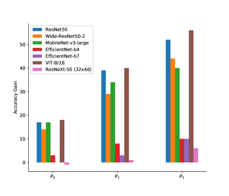
Figure 3: Gains in accuracy of classification of objects on uncommon settings after finetuning on FOCUS.

Input Image

Localization before finetuning

Localization after finetuning

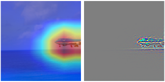
(a) Plane on Water. Base model attends to the water and predicts ‘seashore’, while the Finetuned model correctly predicts ‘warplane’.

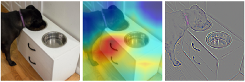
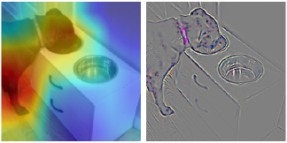
(b) Dog Indoors. Base model predicts ‘dishwasher’. Finetuned model, which localizes on the dog correctly, predicts ‘Labrador Retriever’.

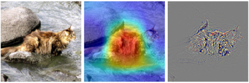
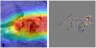
(c) Cat in Water. Base model incorrectly predicts ‘brown bear’. Note the lack of attention on the cat’s head. Finetuned model has a more accurate localization map and predicts ‘tabby cat’.

Figure 4: Comparison of localization maps of a base ResNet50 model (pretrained on ImageNet) before and after finetuning on FOCUS. In each sub-figure, the first image is the input uncommon image. The second and third images, respectively, show the Grad-CAM (Selvaraju et al., 2017) and the Guided Grad-CAM of the model before finetuning. Finally, the fourth and fifth images show the same for the model after finetuning. All Grad-CAM and Guided Grad-CAM images use the predicted class as their target. After finetuning on FOCUS, the model learns to focus more precisely on the object of interest which leads to substantial increase in classification accuracy (see table 3).

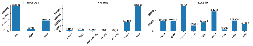
Figure 5: Statistics of various contextual attributes on ImageNet computed by attribute classifiers trained on FOCUS.

4.3 Finetuning

In an attempt to improve classification accuracy in uncommon settings, we finetune the classifiers (except CLIP) we previously tested in subsection 4.2, on the FOCUS dataset. We do not fine-tune CLIP on FOCUS because it is a zero-shot classifier and unlike the other models, it does not have a final fully connected layer that can be fine-tuned. We start by randomly splitting the dataset into train and test sets, which are 70% and 30% of the dataset in size, respectively. We use SGD with a learning rate of 1e-4 to update the last layer (fully-connected layer) of each model for 10 epochs of the train split. Figure 3 shows the gains in top-1 classification accuracy for each of the model on different partitions of the test set. All models perform better on $P_{1}$ and $P_{2}$ after finetuning, with ViT-B/16 having a substantial gain of 40% and 56% respectively. This shows that finetuning on FOCUS improves the generalization of classification models and allows them to identify objects in atypical contexts.

Figure 4 provides some insight into the effects of finetuning a model on FOCUS. The figure compares the localization maps of a base ResNet50 model that was pretrained on imagenet with those of the finetuned model. Each row illustrates an image from the test split of FOCUS that is misclassified by the base model, but is classified correctly by the finetuned model. It also includes the Grad-CAM (Selvaraju et al., 2017) localization maps of both the models on that image. In each case, it is evident that the base model is attending heavily to the wrong part of the image. As a result, it incorrectly predicts a class that is closely associated with the background: (a) In figure 4(a), the model is relying on the presence of water to predict ‘seashore’ even though its in the middle of an sea/ocean (b) In figure 4(b), bowl and the handles on the drawer cause the model to predict a dishwasher (c) Lastly, in figure 4(c), the model only looks at the wet, brown fur in water to predict a ‘brown bear’. On the other hand, the finetuned model focuses more accurately on the correct object alone, allowing it to identify these objects even though they are present in uncommon settings.

4.4 Expanding ImageNet with FOCUS

Although FOCUS has rich sample annotations, its relatively small size prohibits training deep classifiers on it from the scratch. In this section, we show that FOCUS can be effectively used to provide rich annotations for other large-scale and standard image datasets such as ImageNet. To do this, we train three classifiers on FOCUS, one for predicting each of the contextual attributes considered in FOCUS. Specifically, we use a pretrained ResNet50 model as backbone and attach a linear head for $n$-way classification ($n=3,7,9$ for time of day, weather, and location, respectively). To estimate the efficacy of these classifiers on ImageNet, we conducted a separate AMT survey where we ask AMT workers to annotate the contextual attributes for 5,000 randomly chosen images from ImageNet. We find that these classifiers are reasonably accurate: the predictions of the classifier agree with that of the humans 74%, 71%, and 75% of the time, for each of the attributes, respectively.

Finally, we use the attribute classifiers to provide rich annotations of time, weather and location for all ImageNet samples. Figure 5 shows the statistics of various attributes in the train split of ImageNet. Interestingly, we observe that some contexts such as inclement weather and images of objects in the dark are severely underrepresented. Given the wide use of Imagenet in the machine learning community, we believe that such richly annotated version of it can facilitate large-scale future works to improve model generalization. To that end, we will release these annotations on ImageNet, along with the FOCUS dataset upon the acceptance of this paper.

5 Conclusion

In this work, we introduced FOCUS, a dataset that contains images both in common and uncommon settings. FOCUS has around 21K samples annotated by their environmental attributes such as locations, weather, and time of day. Using FOCUS, we evaluated the performance of several popular ImageNet classifiers. These models clearly have reduced performance when classifying images in uncommon settings. We showed that finetuning on our dataset alleviates this issue. We also used FOCUS to machine annotate ImageNet with the attributes mentioned above. We believe that richly annotated datasets such as FOCUS open new directions for the development of deep models that are reliable both in common and uncommon settings.

Appendix

Appendix A Image Search

The images for our dataset were collected using queries formed as a concatenation of an object label and one of the phrases from below:

Attribute	Phrases used in queries
“raining”	“in rain”
“foggy”	“in fog”
“snow”	“on snow”
“sand”	“in a desert”, “on sand”
“forest”	“in forest”
“water”	“on water”
“night”	“at night”
“grass”	“on grass”
“street”	“on a street”, “on a road”

In addition, we use some class specific queries: “ship on ice”, “ship on a dock”, “dog on a couch”, “dog on a bed”, “dog on the floor”, “cat on a couch”, “cat on a bed”, “cat on the floor”, “horse in a stable”, “car in a garage”, “truck in a garage”, “plane in a hangar”.

Figure 6 shows some more uncommon images in FOCUS.

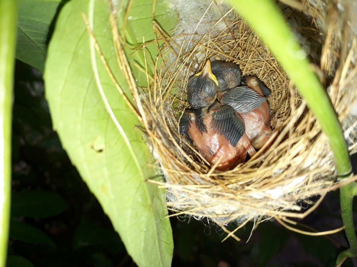
(a) bird at night

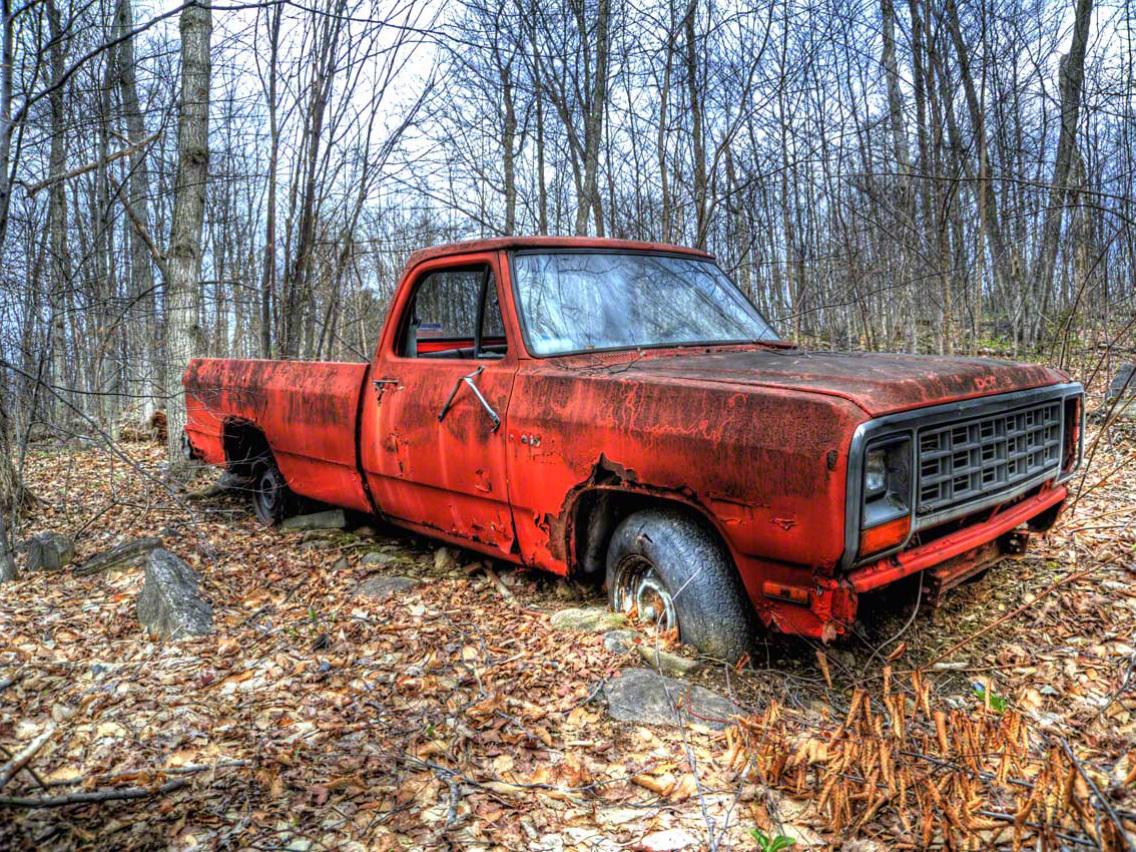
(b) car in forest

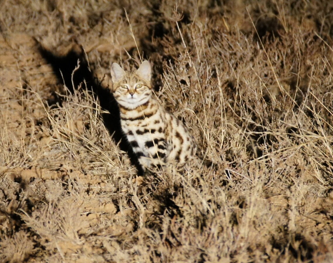
(c) cat at night in forest

(d) plane at night indoors

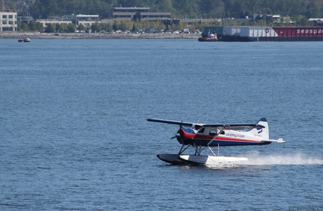
(e) plane in water

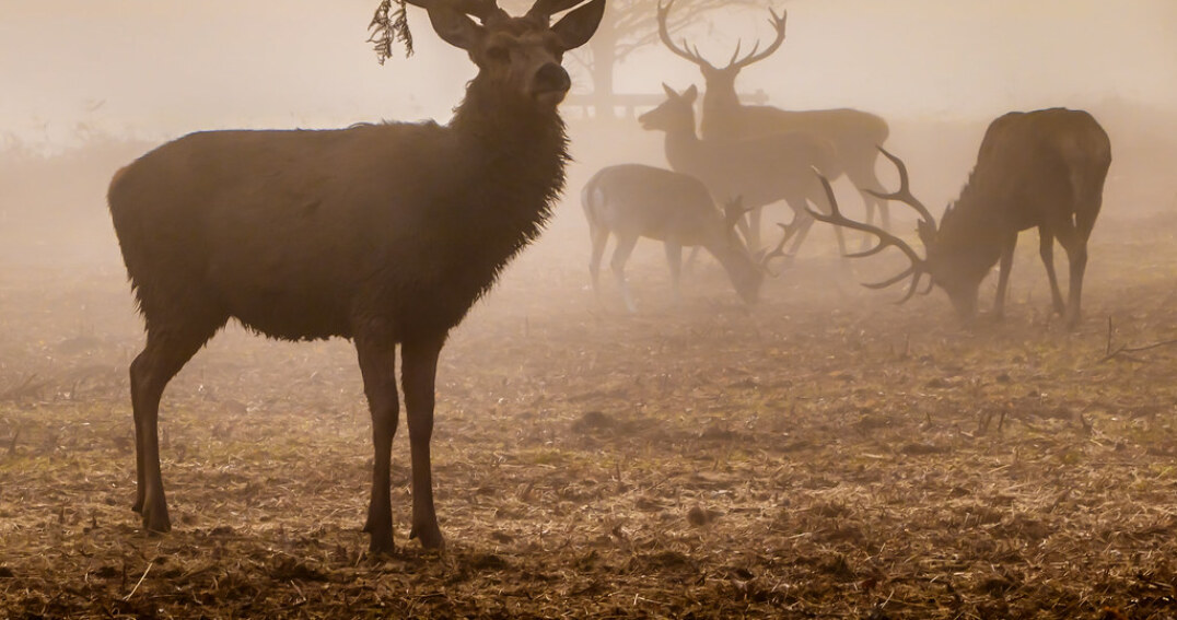
(f) deer in fog

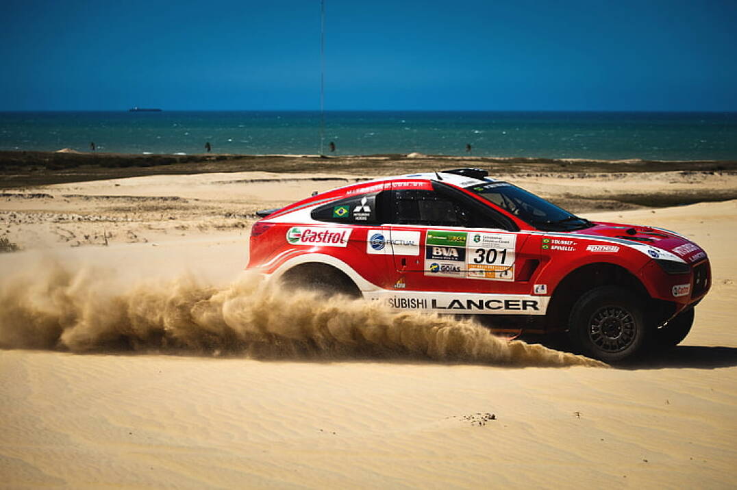
(g) car on sand

(h) dog in snow

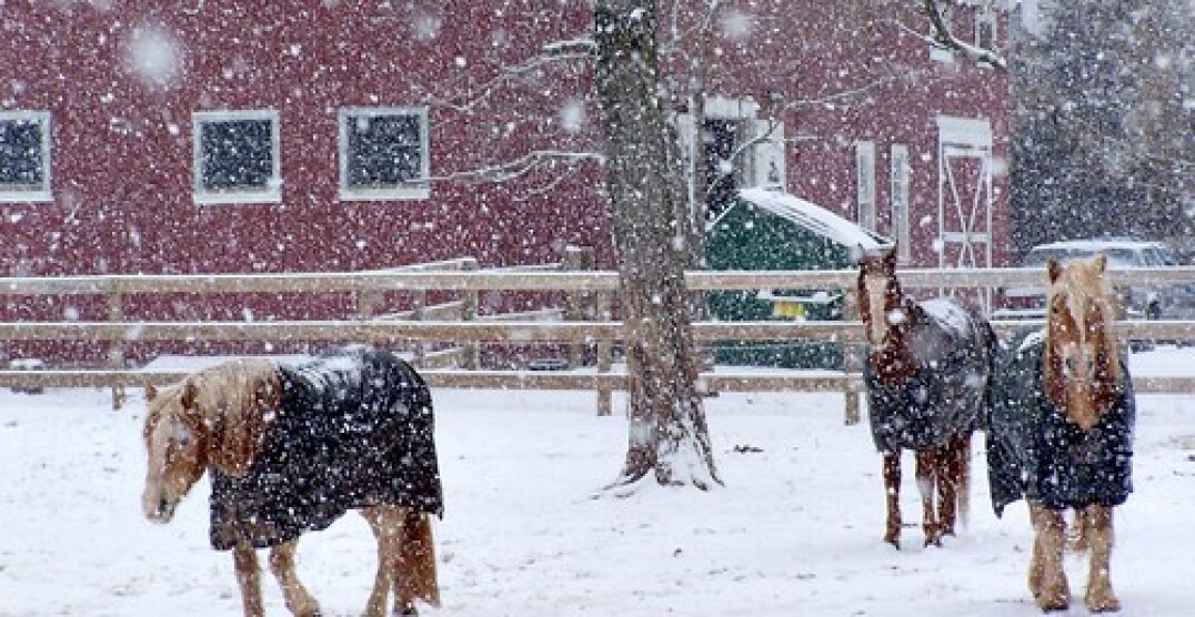
(i) horse in snow

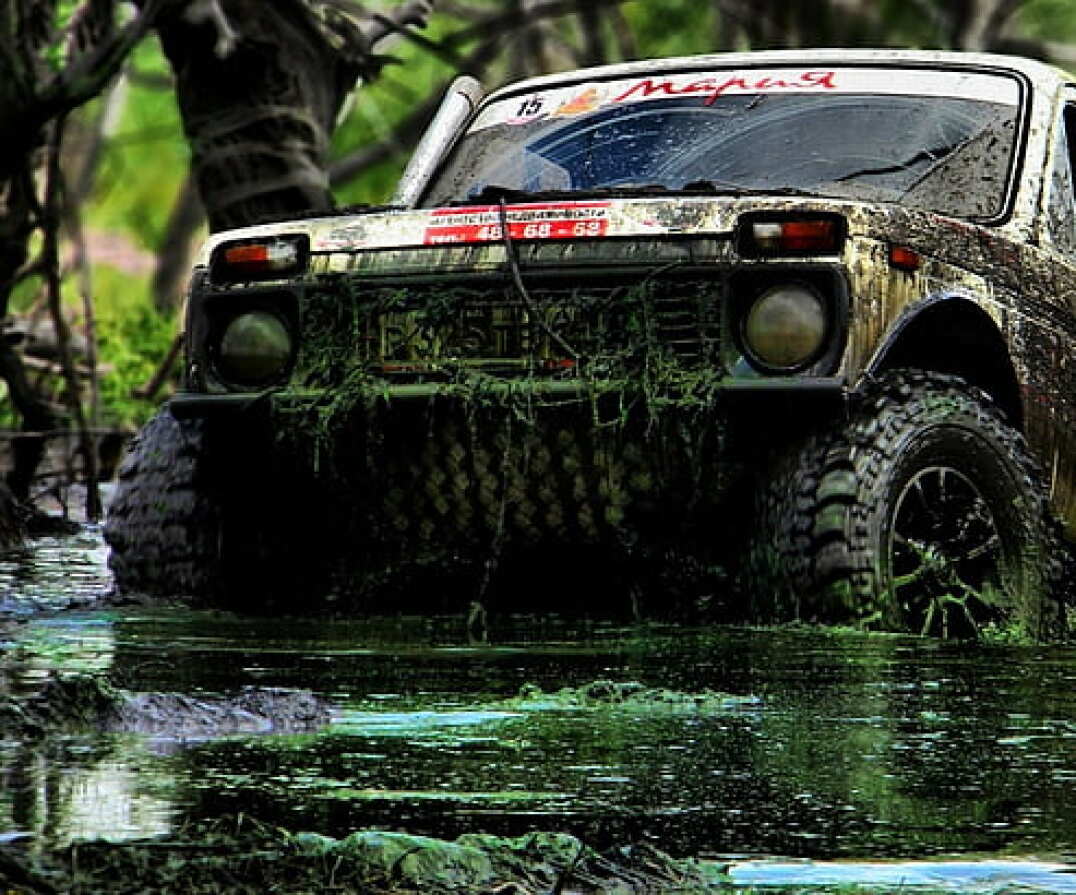
(j) car in water

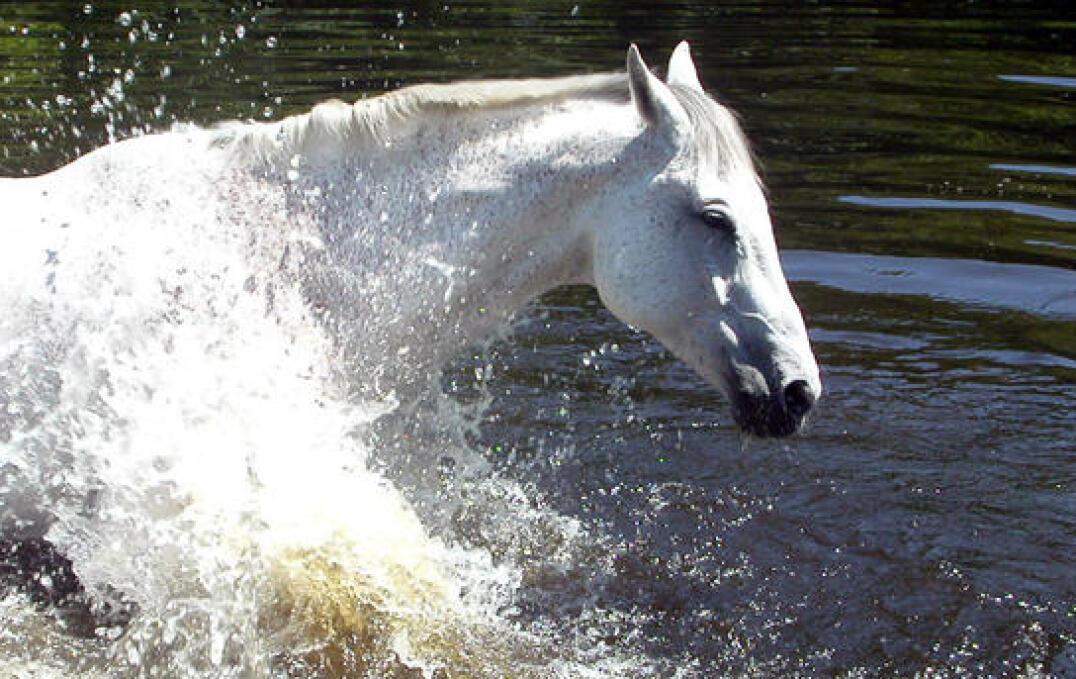
(k) horse in water

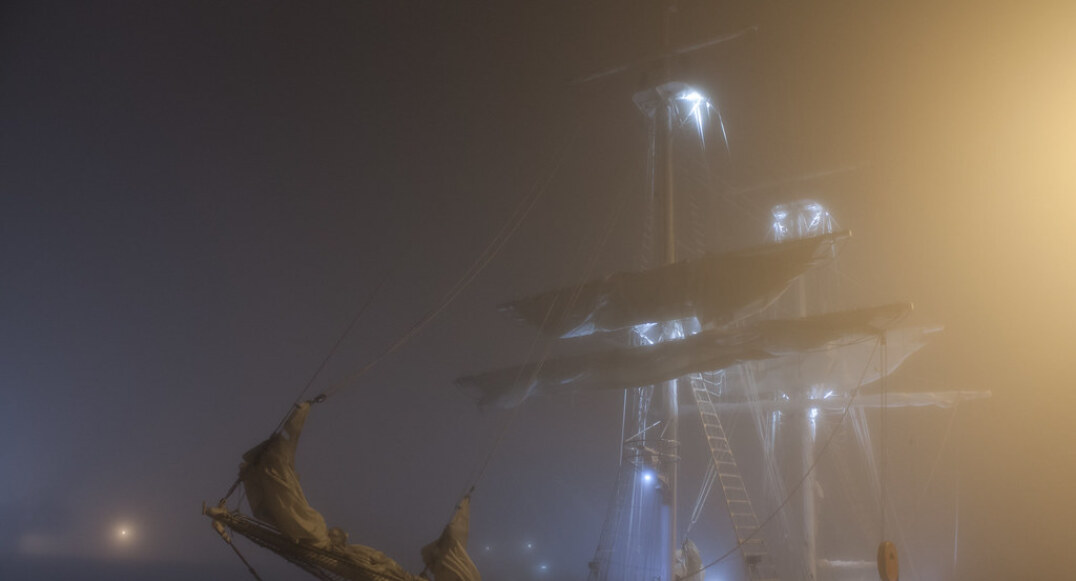
(l) ship in fog

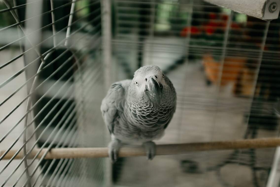
(m) bird indoors

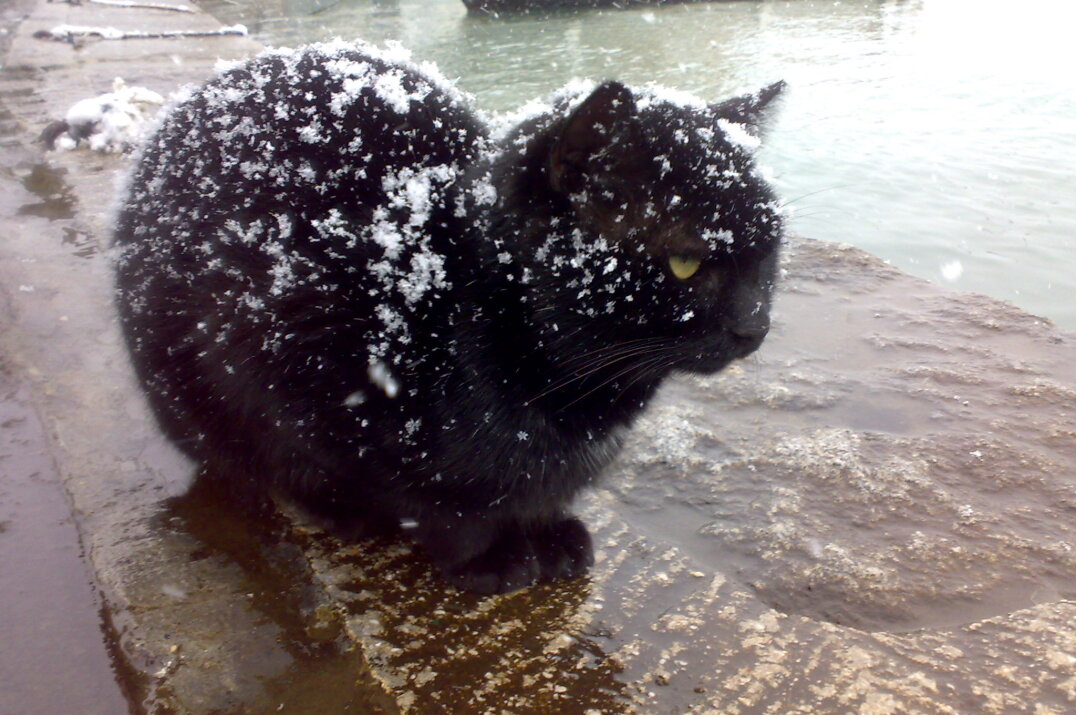
(n) cat in snowy weather & water

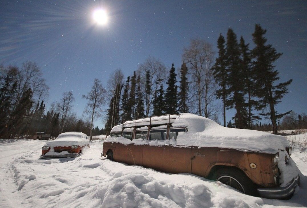
(o) car in snow

Figure 6: Some uncommon images in the FOCUS dataset.

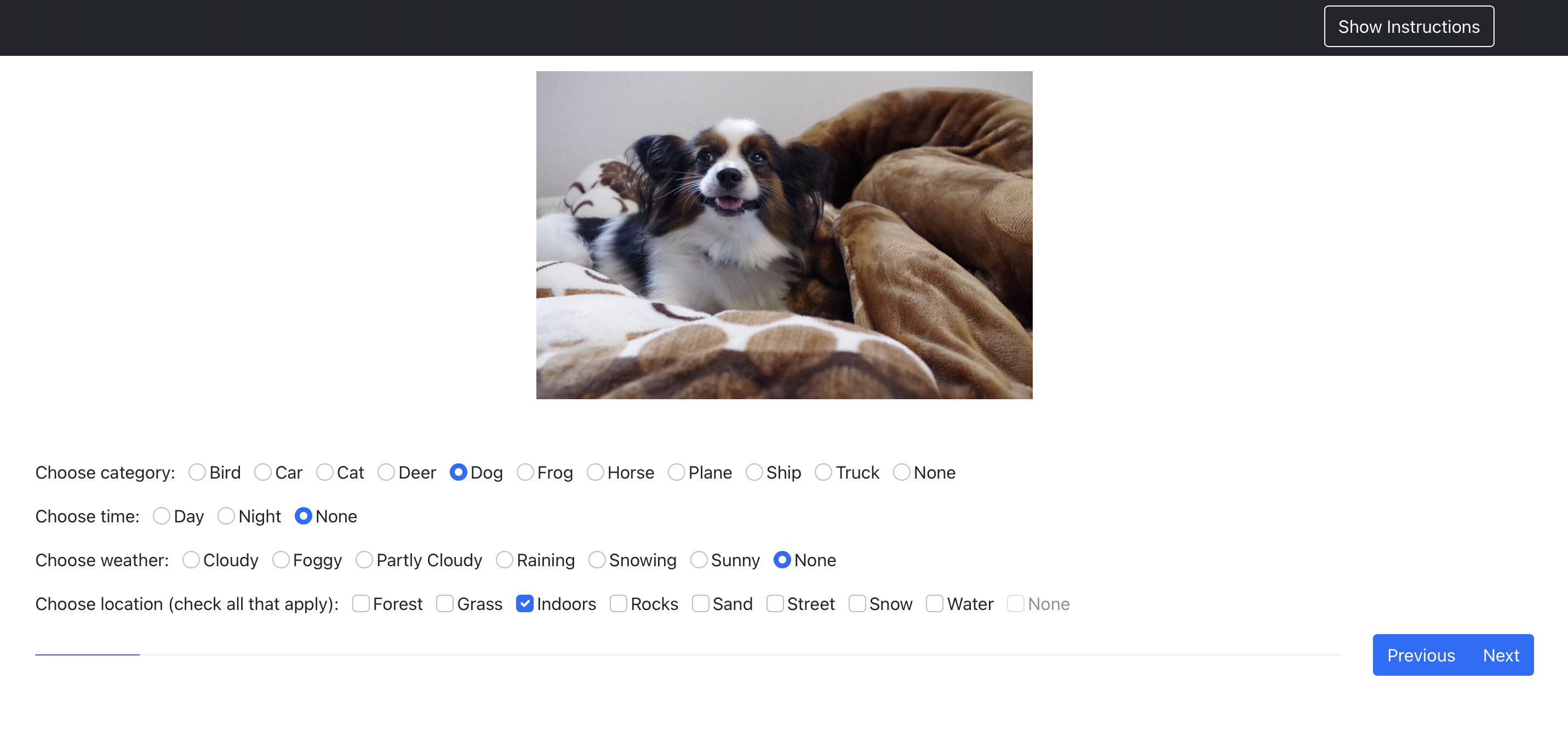
Figure 7: Our UI for annotating images in FOCUS.

Appendix B Human Intelligence Tasks (HITs)

To gather high quality annotations, we first vet the workers through a qualification process; workers are shown a series of 10 images (in the UI shown in figure 7) from our dataset for which the ground truth is known (these images were annotated by us manually). We qualify workers who have done well on this qualification test. Worker’s annotations were checked manually in this stage instead of using a strict threshold as there is an element of subjectivity to the annotations. In the second stage, our HITs have 25 images each; 23 of which are unannotated and 2 are from the subset that were annotated by us. We use these 2 images as a way to track workers’ annotation accuracy. Each image is annotated by two workers and we pick annotations of the worker who has the higher annotation accuracy on the 2 “check” images in that HIT. Workers received a base pay of $0.67 per HIT (25 images) which takes an average of around 5 minutes to annotate. A bonus of $30 was paid for completion of 100 HITs. This payment structure has created an incentive for workers to annotate a large number of images.

Appendix C Accuracy as a function of class and attributes

This section shows the accuracy of different models for each class and attribute. Uncommon attributes are highlighted in shades of orange, while common attributes are highlighted in shades of blue. The last row (except the bottom right-most value) shows the overall accuracy for the corresponding attribute. Additionally, the last column is the generalization gap with respect to the corresponding attribute. The first 10 values in the last column are class specific generalization gaps, while the last (i.e., bottom rightmost) value is the aggregate generalization gap defined in Equation 1 (and reported in table 4).

An image can have a combination of common and uncommon attributes (e.g., “cat on street at night” — uncommon time but common location). Such images may appear in a “blue” cell in one of the tables while in a different table they may appear in “orange”. This explains why for some classes the models seem to do better at “night” than in day. Note that majority of the uncommon weather conditions: (“raining”, “snowing”, “foggy”) occur during the day and they are potentially decreasing the classification accuracy so much that it outweighs the drop due to “night” and leads to this apparently paradoxical result.

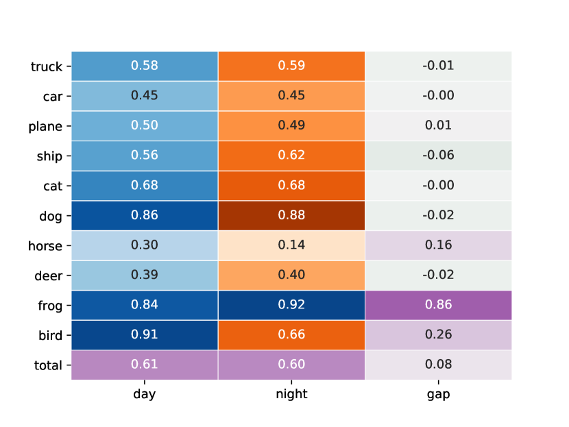
(a) Category vs Time of Day

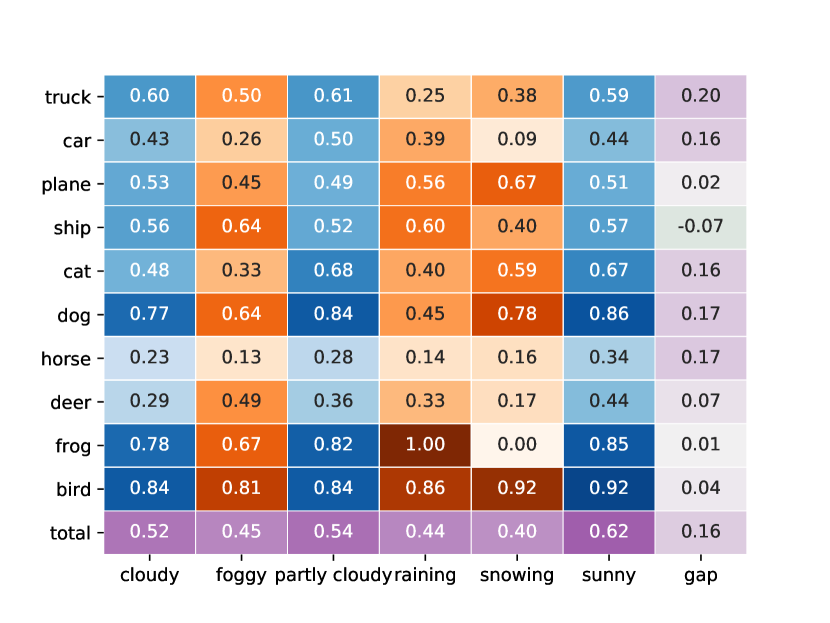
(b) Category vs Weather

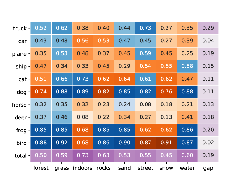
(c) Category vs Location

Figure 8: Accuracy of ResNet50 for all combinations of classes and attributes.

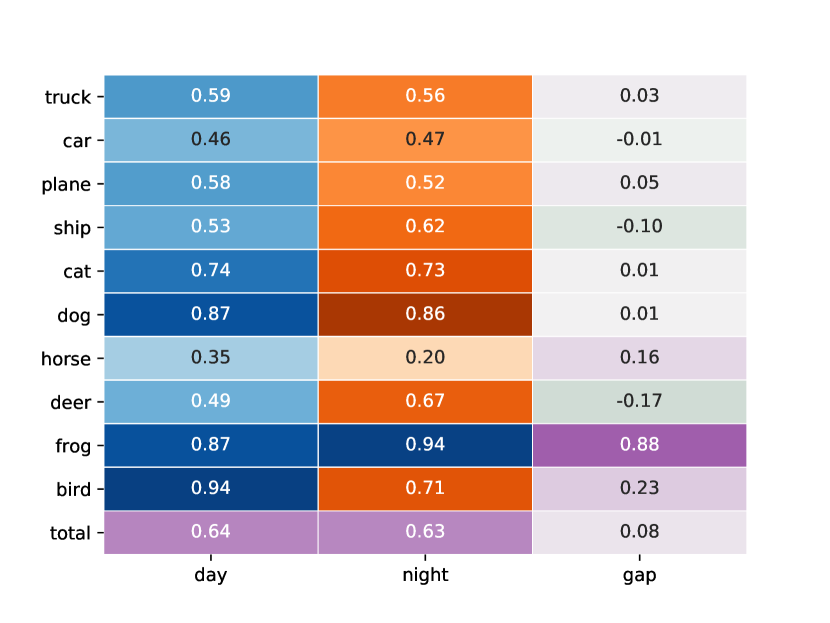
(a) Category vs Time of Day

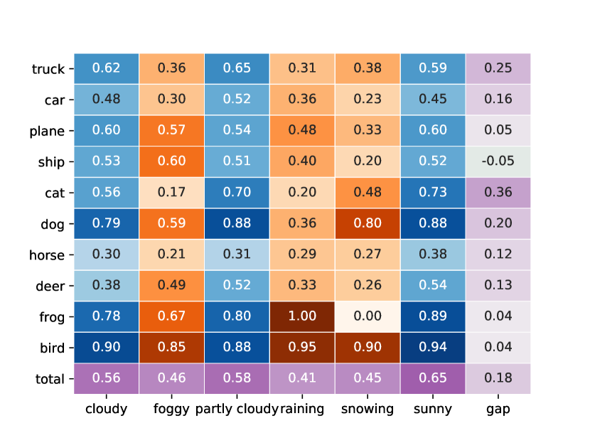
(b) Category vs Weather

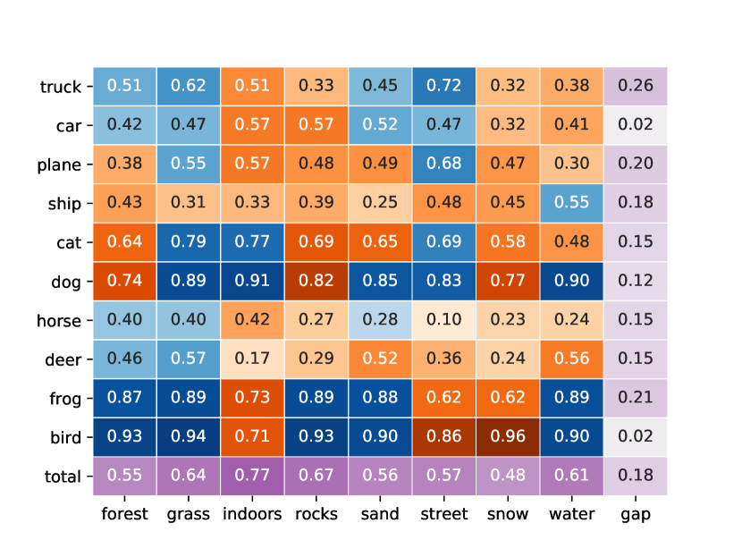
(c) Category vs Location

Figure 9: Accuracy of Wide-ResNet50-2 for all combinations of classes and attributes.

(a) Category vs Time of Day

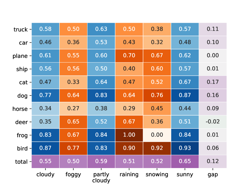
(b) Category vs Weather

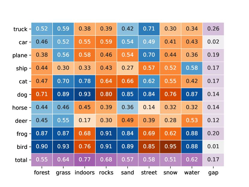
(c) Category vs Location

Figure 10: Accuracy of EfficientNet-b4 for all combinations of classes and attributes.

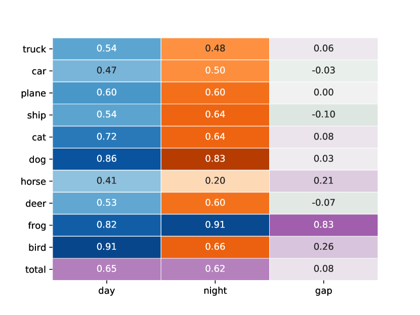
(a) Category vs Time of Day

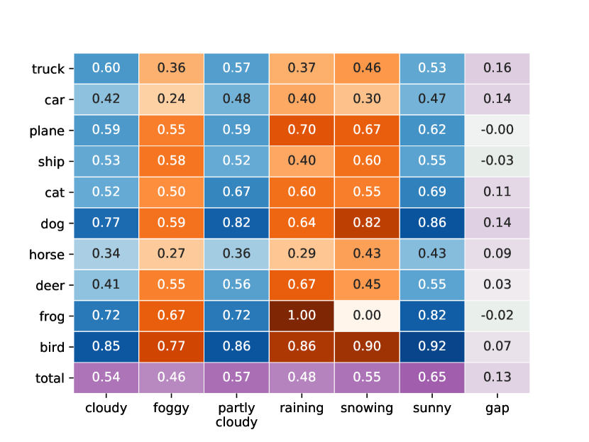
(b) Category vs Weather

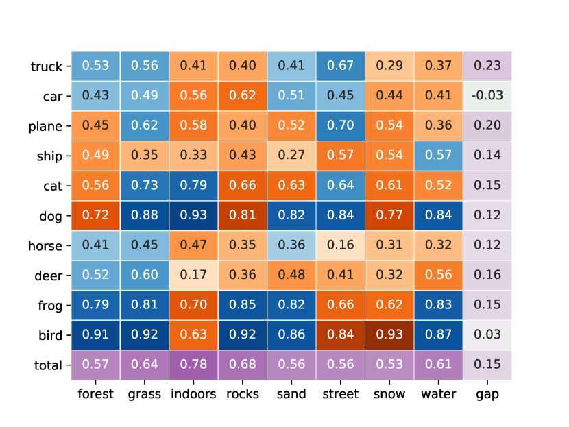
(c) Category vs Location

Figure 11: Accuracy of EfficientNet-b7 for all combinations of classes and attributes.

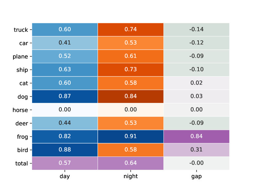
(a) Category vs Time of Day

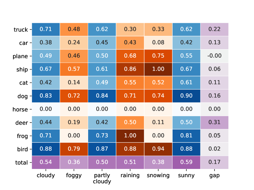
(b) Category vs Weather

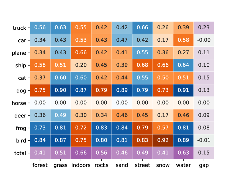
(c) Category vs Location

Figure 12: Accuracy of CLIP for all combinations of classes and attributes.

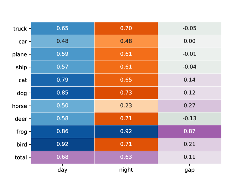
(a) Category vs Time of Day

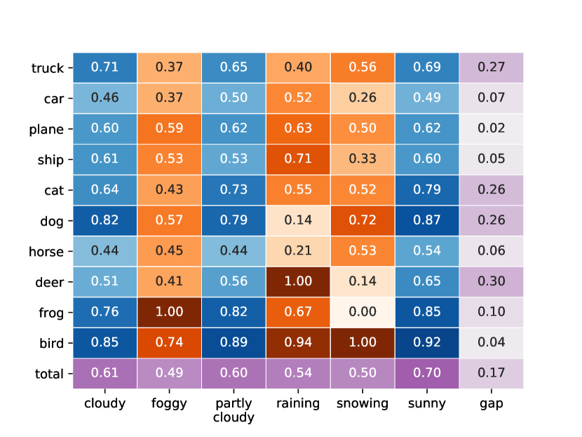
(b) Category vs Weather

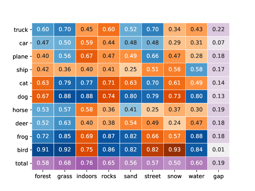
(c) Category vs Location

Figure 13: Accuracy of ViT-B/16 for all combinations of classes and attributes.

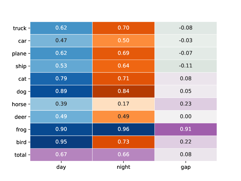
(a) Category vs Time of Day

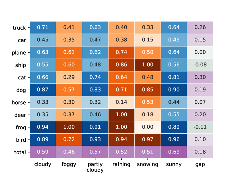
(b) Category vs Weather

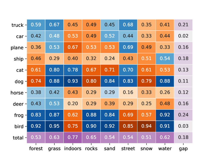
(c) Category vs Location

Figure 14: Accuracy of ResNext-50 (32x4d) for all combinations of classes and attributes.

References

- Barbu et al. (2019) Andrei Barbu, David Mayo, Julian Alverio, William Luo, Christopher Wang, Dan Gutfreund, Josh Tenenbaum, and Boris Katz. Objectnet: A large-scale bias-controlled dataset for pushing the limits of object recognition models. Advances in Neural Information Processing Systems, 32:9453–9463, 2019.
- Beery et al. (2018) Sara Beery, Grant Van Horn, and Pietro Perona. Recognition in terra incognita. In Proceedings of the European conference on computer vision (ECCV), pp. 456–473, 2018.
- Bell et al. (2016) Sean Bell, C. Lawrence Zitnick, Kavita Bala, and Ross Girshick. Inside-outside net: Detecting objects in context with skip pooling and recurrent neural networks. In Proceedings of the IEEE Conference on Computer Vision and Pattern Recognition (CVPR), June 2016.
- Choi et al. (2012) Myung Jin Choi, Antonio Torralba, and Alan S. Willsky. Context models and out-of-context objects. Pattern Recogn. Lett., 33(7):853–862, may 2012. ISSN 0167-8655. doi: 10.1016/j.patrec.2011.12.004. URL https://doi.org/10.1016/j.patrec.2011.12.004.
- Deng et al. (2009) Jia Deng, Wei Dong, Richard Socher, Li-Jia Li, Kai Li, and Li Fei-Fei. Imagenet: A large-scale hierarchical image database. In 2009 IEEE conference on computer vision and pattern recognition, pp. 248–255. Ieee, 2009.
- Divvala et al. (2009) Santosh K. Divvala, Derek Hoiem, James H. Hays, Alexei A. Efros, and Martial Hebert. An empirical study of context in object detection. In 2009 IEEE Conference on Computer Vision and Pattern Recognition, pp. 1271–1278, 2009. doi: 10.1109/CVPR.2009.5206532.
- Dosovitskiy et al. (2021) Alexey Dosovitskiy, Lucas Beyer, Alexander Kolesnikov, Dirk Weissenborn, Xiaohua Zhai, Thomas Unterthiner, Mostafa Dehghani, Matthias Minderer, Georg Heigold, Sylvain Gelly, Jakob Uszkoreit, and Neil Houlsby. An image is worth 16x16 words: Transformers for image recognition at scale. ICLR, 2021.
- Galleguillos et al. (2008) Carolina Galleguillos, Andrew Rabinovich, and Serge Belongie. Object categorization using co-occurrence, location and appearance. In 2008 IEEE Conference on Computer Vision and Pattern Recognition, pp. 1–8, 2008. doi: 10.1109/CVPR.2008.4587799.
- Geirhos et al. (2020) Robert Geirhos, Jörn-Henrik Jacobsen, Claudio Michaelis, Richard Zemel, Wieland Brendel, Matthias Bethge, and Felix A Wichmann. Shortcut learning in deep neural networks. Nature Machine Intelligence, 2(11):665–673, 2020.
- He et al. (2016) Kaiming He, Xiangyu Zhang, Shaoqing Ren, and Jian Sun. Deep residual learning for image recognition. In Proceedings of the IEEE conference on computer vision and pattern recognition, pp. 770–778, 2016.
- Hendrycks & Dietterich (2019) Dan Hendrycks and Thomas Dietterich. Benchmarking neural network robustness to common corruptions and perturbations. Proceedings of the International Conference on Learning Representations, 2019.
- Hendrycks et al. (2021a) Dan Hendrycks, Steven Basart, Norman Mu, Saurav Kadavath, Frank Wang, Evan Dorundo, Rahul Desai, Tyler Zhu, Samyak Parajuli, Mike Guo, Dawn Song, Jacob Steinhardt, and Justin Gilmer. The many faces of robustness: A critical analysis of out-of-distribution generalization. ICCV, 2021a.
- Hendrycks et al. (2021b) Dan Hendrycks, Kevin Zhao, Steven Basart, Jacob Steinhardt, and Dawn Song. Natural adversarial examples. In Proceedings of the IEEE/CVF Conference on Computer Vision and Pattern Recognition (CVPR), pp. 15262–15271, June 2021b.
- Howard et al. (2019) Andrew Howard, Mark Sandler, Grace Chu, Liang-Chieh Chen, Bo Chen, Mingxing Tan, Weijun Wang, Yukun Zhu, Ruoming Pang, Vijay Vasudevan, et al. Searching for mobilenetv3. In Proceedings of the IEEE/CVF International Conference on Computer Vision, pp. 1314–1324, 2019.
- Krizhevsky et al. (2012) Alex Krizhevsky, Ilya Sutskever, and Geoffrey E. Hinton. Imagenet classification with deep convolutional neural networks. In Proceedings of the 25th International Conference on Neural Information Processing Systems - Volume 1, NIPS’12, pp. 1097–1105, Red Hook, NY, USA, 2012. Curran Associates Inc.
- Krizhevsky et al. (2014) Alex Krizhevsky, Vinod Nair, and Geoffrey Hinton. The cifar-10 dataset. online: http://www. cs. toronto. edu/kriz/cifar. html, 55(5), 2014.
- Leclerc et al. (2021) Guillaume Leclerc, Hadi Salman, Andrew Ilyas, Sai Vemprala, Logan Engstrom, Vibhav Vineet, Kai Xiao, Pengchuan Zhang, Shibani Santurkar, Greg Yang, Ashish Kapoor, and Aleksander Madry. 3db: A framework for debugging computer vision models. In Arxiv preprint arXiv:2106.03805, 2021.
- Liu et al. (2015) Ziwei Liu, Ping Luo, Xiaogang Wang, and Xiaoou Tang. Deep learning face attributes in the wild. In Proceedings of International Conference on Computer Vision (ICCV), December 2015.
- Mottaghi et al. (2014) Roozbeh Mottaghi, Xianjie Chen, Xiaobai Liu, Nam-Gyu Cho, Seong-Whan Lee, Sanja Fidler, Raquel Urtasun, and Alan Yuille. The role of context for object detection and semantic segmentation in the wild. In Proceedings of the IEEE Conference on Computer Vision and Pattern Recognition (CVPR), June 2014.
- Oliva & Torralba (2007) Aude Oliva and Antonio Torralba. The role of context in object recognition. Trends in cognitive sciences, 11(12):520–527, 2007.
- Paszke et al. (2019) Adam Paszke, Sam Gross, Francisco Massa, Adam Lerer, James Bradbury, Gregory Chanan, Trevor Killeen, Zeming Lin, Natalia Gimelshein, Luca Antiga, Alban Desmaison, Andreas Kopf, Edward Yang, Zachary DeVito, Martin Raison, Alykhan Tejani, Sasank Chilamkurthy, Benoit Steiner, Lu Fang, Junjie Bai, and Soumith Chintala. Pytorch: An imperative style, high-performance deep learning library. In H. Wallach, H. Larochelle, A. Beygelzimer, F. d'Alché-Buc, E. Fox, and R. Garnett (eds.), Advances in Neural Information Processing Systems 32, pp. 8024–8035. Curran Associates, Inc., 2019.
- Radford et al. (2021) Alec Radford, Jong Wook Kim, Chris Hallacy, Aditya Ramesh, Gabriel Goh, Sandhini Agarwal, Girish Sastry, Amanda Askell, Pamela Mishkin, Jack Clark, et al. Learning transferable visual models from natural language supervision. arXiv preprint arXiv:2103.00020, 2021.
- Rosenfeld et al. (2018) Amir Rosenfeld, Richard Zemel, and John K Tsotsos. The elephant in the room. arXiv preprint arXiv:1808.03305, 2018.
- Russakovsky et al. (2015) Olga Russakovsky, Jia Deng, Hao Su, Jonathan Krause, Sanjeev Satheesh, Sean Ma, Zhiheng Huang, Andrej Karpathy, Aditya Khosla, Michael S. Bernstein, Alexander C. Berg, and Li Fei-Fei. Imagenet large scale visual recognition challenge. International Journal of Computer Vision, 115:211–252, 2015.
- Sagawa* et al. (2020) Shiori Sagawa*, Pang Wei Koh*, Tatsunori B. Hashimoto, and Percy Liang. Distributionally robust neural networks. In International Conference on Learning Representations, 2020. URL https://openreview.net/forum?id=ryxGuJrFvS.
- Sastry & Oore (2020) Chandramouli Shama Sastry and Sageev Oore. Detecting out-of-distribution examples with Gram matrices. In Hal Daumé III and Aarti Singh (eds.), Proceedings of the 37th International Conference on Machine Learning, volume 119 of Proceedings of Machine Learning Research, pp. 8491–8501. PMLR, 13–18 Jul 2020. URL https://proceedings.mlr.press/v119/sastry20a.html.
- Sauer & Geiger (2021) Axel Sauer and Andreas Geiger. Counterfactual generative networks. In International Conference on Learning Representations, 2021. URL https://openreview.net/forum?id=BXewfAYMmJw.
- Selvaraju et al. (2017) Ramprasaath R Selvaraju, Michael Cogswell, Abhishek Das, Ramakrishna Vedantam, Devi Parikh, and Dhruv Batra. Grad-cam: Visual explanations from deep networks via gradient-based localization. In Proceedings of the IEEE international conference on computer vision, pp. 618–626, 2017.
- Singla et al. (2021) Sahil Singla, Besmira Nushi, Shital Shah, Ece Kamar, and Eric Horvitz. Understanding failures of deep networks via robust feature extraction. In Proceedings of the IEEE/CVF Conference on Computer Vision and Pattern Recognition, pp. 12853–12862, 2021.
- Tan & Le (2019) Mingxing Tan and Quoc Le. Efficientnet: Rethinking model scaling for convolutional neural networks. In International Conference on Machine Learning, pp. 6105–6114. PMLR, 2019.
- Wightman (2019) Ross Wightman. Pytorch image models. https://github.com/rwightman/pytorch-image-models, 2019.
- Wong et al. (2021) Eric Wong, Shibani Santurkar, and Aleksander Madry. Leveraging sparse linear layers for debuggable deep networks. In Marina Meila and Tong Zhang (eds.), Proceedings of the 38th International Conference on Machine Learning, volume 139 of Proceedings of Machine Learning Research, pp. 11205–11216. PMLR, 18–24 Jul 2021. URL https://proceedings.mlr.press/v139/wong21b.html.
- Xiao et al. (2020) Kai Xiao, Logan Engstrom, Andrew Ilyas, and Aleksander Madry. Noise or signal: The role of image backgrounds in object recognition. ArXiv preprint arXiv:2006.09994, 2020.
- Xie et al. (2017) Saining Xie, Ross Girshick, Piotr Dollár, Zhuowen Tu, and Kaiming He. Aggregated residual transformations for deep neural networks. In Proceedings of the IEEE conference on computer vision and pattern recognition, pp. 1492–1500, 2017.
- Yu et al. (2020) Fisher Yu, Haofeng Chen, Xin Wang, Wenqi Xian, Yingying Chen, Fangchen Liu, Vashisht Madhavan, and Trevor Darrell. Bdd100k: A diverse driving dataset for heterogeneous multitask learning. In Proceedings of the IEEE/CVF conference on computer vision and pattern recognition, pp. 2636–2645, 2020.
- Zagoruyko & Komodakis (2016) Sergey Zagoruyko and Nikos Komodakis. Wide residual networks. arXiv preprint arXiv:1605.07146, 2016.