Optimal SNR Analysis for Single-user RIS Systems in Ricean and Rayleigh Environments
Abstract
We present an analysis of the optimal uplink (UL) SNR of a SIMO Reconfigurable Intelligent Surface (RIS)-aided wireless link. We assume that the channel between base station (BS) and RIS is a rank-1 LOS channel while the user (UE)-RIS and UE-BS channels are correlated Ricean. For the optimal RIS matrix, we derive an exact closed form expression for the mean SNR and an approximation for the SNR variance leading to an accurate gamma approximation to the distribution of the UL SNR. Furthermore, we analytically characterise the effects of correlation and the Ricean K-factor on SNR, showing that increasing the K-factor and correlation in the UE-BS channel can have negative effects on the mean SNR, while increasing the K-factor and correlation in the UE-RIS channel improves system performance. We also present favourable and unfavourable channel scenarios which provide insight into the sort of environments that improve or degrade the mean SNR. We also show that the relative gain in the mean SNR when transitioning from an unfavourable to a favourable environment saturates to as .
I Introduction
Reconfigurable Intelligent Surface (RIS) aided wireless networks are currently the subject of considerable research attention due to their ability to manipulate the channel between users (UEs) and base station (BS) via the RIS. Assuming that channel state information (CSI) is known at the RIS, one can intelligently alter the RIS phases, essentially changing the channel to improve system performance. Here, we focus on a single user system and assume a common system scenario where a RIS is carefully located near the BS such that a rank-1 line-of-sight (LOS) channel is formed between the BS and RIS. System scenarios with a LOS channel between the BS-RIS and a single-user are also considered in [1, 2, 3, 4] with motivation for the LOS assumption given in [3]. All of these existing works aim to enhance the system to achieve some optimal system performance (sum rate, SINR, etc.) by tuning the RIS phases. In particular, [3] gives a closed form RIS phase solution without the presence of a direct UE-BS channel for a single user setting, while [4] gives a closed form phase solution with the presence of a direct channel. We note, however, once the optimal RIS has been defined there is no exact analysis of the mean SNR and no analysis of correlation impact on the mean SNR in [1, 2, 3, 4].
For the UE to RIS and the direct UE to BS links, the presence of scattering is a more reasonable assumption as is spatial correlation in the channels, especially at the RIS where small inter-element spacing may be envisaged. Several papers do consider spatial correlation in the small-scale fading channels [3, 5, 6, 7, 8, 9, 10, 11], however, these papers are simulation based and no analysis is given on the impact of correlation on the mean SNR.
Statistical properties of the RIS-aided channel have been investigated in existing literature. For example, [12, 13] provide a closed form expression for the mean SNR in the absence of a UE-BS channel with [13] additionally providing a probability density function (PDF) and a cumulative distribution function (CDF) for the distribution of the mean SNR. In [12, 14], an upper bound is given for the ergodic capacity and in [15] a lower bound is given for the ergodic capacity. However, there are no closed form expressions for the mean SNR and SNR variance for an optimum RIS-aided wireless system, in the presence of correlated Ricean UE-BS, UE-RIS fading channels. We further note that the work presented in this paper is an extension for the work done in [16] which considered correlated Rayleigh UE-BS, UE-RIS fading channels.
In this paper, we focus on an analysis of the optimal uplink (UL) SNR for a single user RIS aided link with a rank-1 LOS RIS-BS channel and correlated Ricean fading for the UE-BS and UE-RIS channels. The contributions of this paper are as follows:
-
•
An exact closed-form result for mean SNR and an approximate closed form expression for SNR variance are derived. These are used to show that a gamma distribution provides a good approximation of the UL optimal SNR distribution. Furthermore, using the analysis presented, we are able to reduce the mean SNR and SNR variance expressions when the UE-BS and UE-RIS links are correlated Rayleigh to agree with those in [16].
-
•
The analysis is leveraged to gain insight into the impact of the K-factor and spatial correlation on the mean SNR. We show that increasing the K-factor and correlation in the UE-BS channel has negative effects, while increasing the K-factor and correlation in the UE-RIS channel improves the mean SNR.
-
•
Given the analyses, we present favourable and unfavourable channel scenarios, which provide insight into the sort of environments that would improve and degrade the mean SNR. For systems with a large number of RIS elements, we show that when changing from favourable to unfavourable channel scenarios, improvements in the mean SNR saturate at a relative gain of as .
Notation: represents statistical expectation. is the Real operator. denotes the norm. Upper and lower boldface letters represent matrices and vectors, respectively. denotes a complex Gaussian distribution with mean and covariance matrix . denotes a uniform random variable taking on values between and . denotes a chi-squared distribution with degrees of freedom. represents an matrix with unit entries. The transpose, Hermitian transpose and complex conjugate operators are denoted as , respectively. The trace and diagonal operators are denoted by and , respectively. The angle of a vector of length is defined as and the exponent of a vector is defined as . denotes the Kronecker product. denotes a Laguerre function of non-integer degree .
II System Model
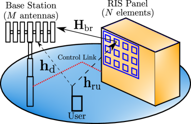
As shown in Fig. 1, we examine a RIS aided single user single input multiple output (SIMO) system where a RIS with reflective elements is located close to a BS with antennas such that a rank-1 LOS condition is achieved between the RIS and BS.
II-A Channel Model
Let , , be the UE-BS, UE-RIS and RIS-BS channels, respectively. The diagonal matrix , where for , contains the reflection coefficients for each RIS element. The global UL channel is thus represented by
| (1) |
where we consider the correlated Ricean channels:
with
where and are the link gains between UE-BS and UE-RIS respectively, and are the correlation matrices for UE-BS and UE-RIS links, respectively, and . Here, and are the Ricean K-factors for the UE-BS and UE-RIS channels, respectively. The LOS paths and are topology specific steering vectors at the BS and RIS respectively. Particular examples of steering vectors for a vertical uniform rectangular array (VURA) are given in Sec. V.
Note, that the correlation matrices and can represent any correlation model. For simulation purposes, we will use the well-known exponential decay model,
| (2) |
where , . is the distance between the and antenna/element at the BS/RIS. and are the nearest-neighbour BS antenna separation and RIS element separation, respectively, which are measured in wavelength units. and are the nearest neighbour BS antenna and RIS element correlations, respectively.
The rank-1 LOS channel from RIS to BS has link gain and is given by where and are topology specific steering vectors at the BS and RIS, respectively.
II-B Optimal SNR
Using (1), the received signal at the BS is, where is the transmitted signal with power and . For a single user, Matched Filtering (MF) is the optimal combining method so the optimal UL SNR is, where . The optimal RIS phase matrix to maximize the SNR can be computed using the main steps outlined in [4, Sec. III-B] but using an UL channel model instead of downlink. Substituting the channel vectors and through some matrix algebraic manipulation, the optimal RIS phase matrix is,
| (3) |
Substituting (3) into , the optimal UL global channel is,
| (4) |
where , giving the optimal UL SNR as
| (5) |
where and . The variable is given its own notation as it arises in many of the derivations for the SNR.
III Mean SNR and SNR Variance
III-A Correlated Ricean Channels
Here, we provide an exact closed form result for and an exact expression for when and are correlated Ricean channels. Utilising these expressions, we then show that they can be reduced to the expressions given in [16] when and are correlated Rayleigh channels.
Theorem 1.
The mean SNR is given by
| (6) |
with given by
| (7) |
and , where , is the confluent hypergeometric function, , , , and is given by and for [17, Eq. (26b)].
The formula for the mean SNR in (1) is compact and intuitive except for the term which is easier to understand from its definition in App. A as
| (8) |
Note that evaluation of requires the product moment of two correlated Ricean variables. While compact expressions are given in [18] for the PDF of two correlated Ricean variables, it is important to note that these PDFs are for the special case where the LOS components are the same. Here, there is a phase shift that occurs between any two RIS elements and this assumption cannot be made. Hence, we have used the more general bivariate Ricean distribution in [17]. When the UE-RIS channel is non-LOS (correlated Rayleigh) then the complexity in all the expressions reduces considerably.
Theorem 2.
The SNR Variance is given by
| (9) |
with
| (10) | |||
| (11) | |||
| (12) |
| (13) | |||
| (14) | |||
| (15) |
where is given in Theorem 1, is given by (1), , , is the Whittaker M function, and .
In (2), all terms are known except for and . To the best of our knowledge, these moments are intractable and approximations are required for these moments. Note that is positive, unimodal, and the sum of random variables. A gamma distribution is commonly used to approximate such distributions, eg., [12]. Since the first and second moments of are known exactly, we are able to fit a gamma approximation to with the correct first and second moments. Using this gamma approximation, we obtain approximations for and as presented in the following Corollary,
Corollary.
Note that for high values of correlation and the K-factor, (1) is computationally expensive as in such scenarios the number of terms required in the double summation over and grows large. In these situations, an alternative approach is to replace the double summation with its integral equivalent, derived in App. F, and presented in the following cases where and . The case of perfect correlation, , provides a useful benchmark to evaluate the SNR trends as the level of correlation increases.
III-B Case 1: for
| (17) |
where , , and .
III-C Benchmark Case: when
For the benchmark case of maximum correlation, , both (1) and (III-B) result in an indeterminate answer. However, we can use the integral form of and find its result as which, using the derivation in App. F, gives
| (18) |
where and are defined in Sec. III-B. Note that the double numeric integrations required in (III-B) and (III-C) are computationally convenient as: one integral is finite range and the integrand is smooth and rapidly decaying as .
III-D Special Case 1: Uncorrelated Ricean Case
For independent Ricean fading, we provide exact closed form expressions for both and . The mean SNR is given by
| (19) |
with given by
| (20) |
This can be easily derived from Theorem 1 by noting that is the sum of products of iid Ricean random variables over all for and since and .
The SNR Variance is given by
| (21) |
with
| (22) | |||
| (23) | |||
| (24) |
| (25) | |||
| (26) | |||
| (27) | |||
| (28) | |||
| (29) |
Equations (III-D)-(29) follow from Theorem 2 using the substitutions , , and the version of given in (20). A consequence of having uncorrelated UE-BS and UE-RIS channels, is that the expectations and are known exactly and these are given by (28) and (29) respectively.
III-E Special Case 2: Correlated Rayleigh Case
We obtain mean SNR and SNR variance expressions for correlated Rayleigh channels and by setting .
III-E1 Mean SNR
Note that when , and . Similarly when , and . As such, the second term in (1) reduces down to the second term in [16, Eq. (8)]. The third term can be reduced to its correlated Rayleigh form as shown in [16, Eq. (8)] by reducing to (31) (see App. E). The final form after reducing all of the terms in (1) results in the mean SNR expression in [16, Eq. (8)]; given below for completeness:
Theorem 3.
The mean SNR when and are correlated Rayleigh channels is given by
| (30) |
with given by
| (31) |
and , where is the Gaussian hypergeometric function and .
III-E2 SNR Variance
In addition to the steps undertaken in III-E1, we further note that . This eliminates many of the terms in (2) of Theorem 2. Using App. E to collapse down to its correlated Rayleigh form, we obtain the final SNR variance expression for correlated Rayleigh channels, consistent with that given in [16, Eq. (10)] and given below for completeness:
Theorem 4.
The SNR variance when and are correlated Rayleigh channels is given by
| (32) |
where , is given by (31), is given in Theorem 1 and .
Corollary.
To obtain an SNR variance approximation in closed form, we approximate the 3, 4 moments of by,
| (33) |
with
where is given by (31).
IV Performance Insights based on
Note that the first term in the mean SNR in (1) is influenced by variants of the function for , , where the factor of arises from the and terms. Hence, we study the behaviour of before developing performance insights based on the mean SNR.
IV-A Behaviour of
Using [19, Eq. (13.6.9)] the Laguerre function can be rewritten in terms of the confluent hypergeometric function, , as
| (34) |
Using the series expansion for [19, Eq. (13.1.2)] and the Maclaurin series expansion of , we have the following expansion for ,
First, we look at the behaviour near the origin. Noting that , then for , is increasing in and for , is decreasing in .
Next, we look at the behaviour as . Using the asymptotic behaviour of [19, Eq. (13.1.5)], we have
| (35) | ||||
| (36) |
From (35), we see that as , for and for . Differentiating (35) and simplifying gives
| (37) |
for large values of . From (37), we make the following observations. As , for and for .
Collating these properties, we obtain the following result:
Result 1.
The main characteristics of are given by
IV-B Effect of on
Only the first and third terms in (1) are affected by . The first term contains so is increasing with from Result 1. In the third term, affects the mean SNR via the expression. Applying Hölders inequality [20, E.q. (1.1)] to in (8) gives . This upper bound is achieved when . Hence, we conclude that increasing improves the mean SNR.
IV-C Effect of on
Only the first term in (1) is affected by through the expression
From Result 1, this expression increases with when , decreases when and has a more complex behavior in-between.
This pattern can be explained by the fact that measures the alignment of the RIS-BS channel, , with the LOS component of the direct path, , while measures the alignment of with the scattered component of the direct path. Hence, when the RIS-BS aligns strongly with the direct LOS path then improves the SNR. Conversely, when the RIS-BS aligns strongly with the direct scattered channel then increasing reduces the SNR.
The dominant efect here is the case, where decreases the mean SNR. This is because it is unlikely for two independent steering vectors to strongly align, whereas can align with in several ways as the correlation matrix is usually full-rank (see [16]).
IV-D Effect of on
The effect of correlation in the UE-RIS channel, , on the mean SNR is confined to the variable in (1). Identifying the behavior of with respect to is very difficult due to the oscillations in the series expansion given in (1) caused by the term.
However, when we have the correlated Rayleigh case and becomes in (31) which increases with correlation (see [16]). Hence, we conjecture the same broad trend here, so that the mean SNR usually benefits from increasing correlation in .
It is worth noting that the majority of the existing literature does not have the complication of the term in the bivarate Ricean PDF. This is due to the assumption that both of the Ricean variables have identical LOS components (see [18] for example). However, this simplifying assumption is not valid here and the more complex version in [17] is required.
IV-E Effect of on
IV-F Favourable and Unfavourable Conditions
From Sec. IV-B - Sec. IV-E, low correlation and low K-factor in the UE-BS link along with a high K-factor in the UE-RIS link tend to improve . Hence, we define the favourable channel scenario as an iid Rayleigh channel between UE and BS and pure LOS between UE and RIS. Conversely, the unfavourable channel scenario comprises an iid Rayleigh UE-RIS channel and a LOS UE-BS channel.
Using the analysis in Sec. IV, the mean SNR in the favourable channel scenario is given by,
| (38) |
while the mean SNR in the unfavourable channel scenario is,
| (39) |
using the result for for uncorrelated Rayleigh fading (see [16, Eq. (14)]).
Next we consider the relative difference between these two scenarios for large RIS sizes. Defining the gain
| (40) |
it is straightforward to show that
Hence, for large RIS, the asymptotic relative gain between the channel scenarios is approximately 27.32%.
In order to find the maximum gain, we rewrite (40) as
| (41) |
V Results
We present numerical results to verify the analysis in Sec. IV. Firstly, note that we do not consider cell-wide averaging as the focus is on the SNR distribution over the fast fading. Furthermore, the relationship between the SNR and the path gains, and , is straightforward, as shown in (1). Hence, we present numerical results for fixed link gains. In particular, since the RIS-BS link is LOS, we assume where m. Next, for simplicity, . This was chosen to give the 95%-ile of the SNR distribution as 25 dB in the baseline case of moderate channel correlation and identical Ricean K-factors for the LOS and scattered paths (defined as , ), with BS antennas and RIS elements.
As stated in Sec. II-A, the steering vectors for are not restricted to any particular formation. However, for simulation purposes, we will use the VURA model as outlined in [21], but in the plane with equal spacing in both dimensions at both the RIS and BS. The and components of the steering vector at the BS are and which are given by
respectively. Similarly at the RIS, and are defined by,
respectively, where , with being the number of antenna columns and rows at the BS and being the number of columns and rows of RIS elements, , , where and are in wavelength units. The steering vectors at the BS and RIS are then given by,
| (42) |
respectively. and are elevation/azimuth angles of arrival (AOAs) at the BS and are the corresponding angles of departure (AODs) at the RIS. The elevation/azimuth angles are selected based on the following geometry representing a range of LOS links with less elevation variation than azimuth variation: . For all results in this paper we use a single sample from this range of angles given by .
For the LOS components in the UE-BS and UE-RIS channels, the and components of the steering vector at the BS are and which are given by
respectively. Similarly at the RIS, and are defined by,
respectively. Therefore, the LOS components in the UE-BS and UE-RIS channels are given by,
| (43) |
where and are elevation/azimuth angles of arrival (AOAs) for the UE at the BS and are the corresponding angles of departure (AODs) for the UE at the RIS. For all results in this paper we use a single sample of angles from , which are given by .
Note that all of these parameter values and variable definitions are not altered throughout the results and figures, unless specified otherwise.
V-A Approximate CDF for SNR
It is known that the SNR of a wide range of fading channels can be approximated by a mixture gamma distribution [22]. Also, as discussed in Sec. III, it is well-known that a single gamma approximation is often reasonable for a sum of a number of positive random variables [12]. Motivated by this, we approximate the SNR in (5) by a single gamma variable.
The shape parameter of a gamma approximation to the SNR is given by and the scale parameter is , where and are given in Sec. III. Using these values of , the analytical and simulated SNR CDFs are shown in Fig. 2 for and , both with and . When computing the analytical SNR CDFs, for , (III-D) and (III-D) were used but with presented in Sec. III-D. For , (1) and (2) were used. For , (1) and (2) were also used but with given by (III-B).
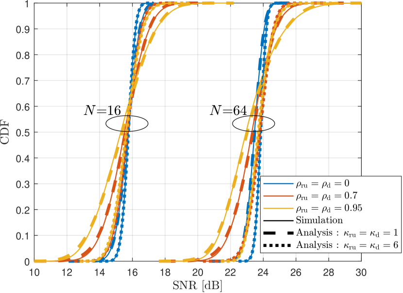
As expected, there is a very good agreement between the simulated and analytical SNR CDFs when due to exact mean SNR and SNR variance expressions being available for all and . For higher correlation, we can see that that the agreement deviates slightly in the lower and upper tails when the K-factor is small. This is due to the approximation made by fitting a gamma distribution using the 3rd and 4th moments of . For higher K-factors, the 3rd and 4th moments of are better approximated due to the UE-RIS channel being dominated by the LOS path, which will cause to be close to deterministic. In such scenarios, the gamma distribution provides an even better representation of the UL SNR. In general, for all correlation and K-factor scenarios, the gamma distribution provides a good representation of the UL SNR even in high correlation scenarios.
V-B The effects of and Asymptotic Results
Here, we verify the performance insights based on described in Sec. IV. Fig. 3 gives the SNR simulations and analyses for various correlation and K-factor combinations in and . As a general observation, it is apparent that the analysis agrees with the simulations for every scenario.
Inspection of Fig. 3 reveals that increasing has a negative impact on the mean SNR as predicted by the analysis. The analysis also predicted that correlation in the direct channel negatively impacts performance, which is also seen in Fig. 3. The best performance occurs for , which supports the favourable channel scenario claim in the analyses. Finally, the worst performance is observed when , supporting the unfavourable channel scenario claim in Sec. IV.
Furthermore, although not visible, scenarios where the channel has a very high K-factor will yield very similar curves regardless of the correlation in that channel. For example, the curve for is very similar to the curve for . This observation is not unusual since the channel is dominated by the LOS path and is thus not significantly impacted by scattering.
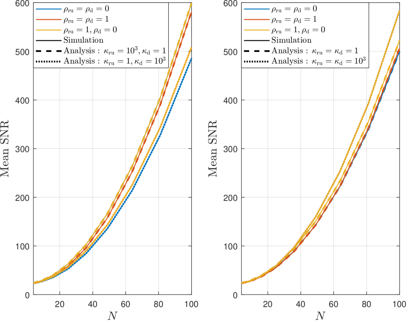
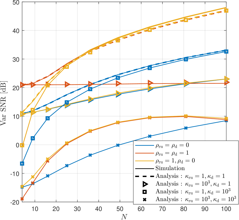
Fig. 4 shows the accuracy of the SNR variance approximation. As expected, for scenarios where and are uncorrelated, we note perfect agreement between the simulations and analyses. As the K-factor in the UE-RIS channel, , increases, the variance is reduced, which becomes significant when both and are very large. This effect is also observed by the change in the CDF spread in Fig. 2.
For scenarios where the K-factor is low, the accuracy of the agreement between simulation and analyses is a consequence of the approximations of the 3rd and 4th moments of only, since all of the other terms in the expression can be expressed in closed form. From Fig. 4 it can be seen that as the number of RIS elements increases, the approximation worsens for highly correlated scenarios with and . However, for the identical correlation scenarios with and , the approximation improves. Note that is the sum of amplitudes of the correlated elements in . When the K-factor is very high, then and , hence the observed improvement in the approximation.
The convergence of the various curves in Fig. 4 supports the claim in the analyses that increasing the number of RIS elements reduces the negative impacts of and in the UE-BS channel. This is seen in the curves relating to and as well as the curves relating to and .
Finally, we verify the results regarding the relative gain given in Sec. IV. The relative gain improvement in (40), when transitioning from unfavourable to favourable channel scenarios, is simulated for a range of different link gains and shown in Fig. 5.
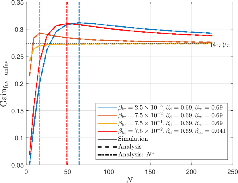
As can be seen, all of the different link gain scenarios asymptotically approach as per the analysis and the saturation rate is dependent on the link gain values. Also apparent is that having a large number of RIS elements does not always yield the maximum relative gain. The vertical lines represent the number of RIS elements required to achieve the maximum possible gain, as detailed in Sec. IV-F. In general, the simulation and analysis agree.
VI Conclusion
We derive an exact closed form expression for the mean SNR of the optimal single user RIS design where spatially correlated Ricean fading is assumed for the UE-BS and UE-RIS channels and the RIS-BS channel is LOS. We also provide an accurate approximation of the SNR variance and a gamma approximation to the CDF of the SNR. Furthermore, we show that when the UE-RIS and UE-BS channels are correlated Rayleigh, both the mean SNR and SNR variance expressions under correlated Ricean channels can be reduced to the expressions given in [16]. The analysis presented offers new insight into how spatial correlation and the Ricean K-factor impact the mean SNR and scenarios in which we would expect high and low SNR performance. Specifically, we show that the mean SNR benefits from having a high correlation and a high K-factor in UE-RIS channel while the UE-BS channel has low correlation and a low K-factor. These correlation and K-factor extremes represent favorable channel scenarios while unfavorable channel scenarios occur at the opposite ends of these extremes. To this end, we show that the asymptotic gain achievable when transitioning between unfavourable and favourable environments is .
Appendix A Derivation of mean SNR
Expanding (5) gives,
| SNR | |||
We compute by computing the expectation of each term in the expression above.
Term 2: Substituting from Sec. II-B into ,
Firstly, we can rewrite the definition of the element of in Sec. II-A as where and . Then using the moments of a Ricean RV [24, Eq. (2.3-58)] and a confluent hypergeometric to Laguerre polynomial relation [19, Eq. (13.6.9)], we have
Similarly,
where . Therefore,
| (45) |
Appendix B Derivation of SNR Variance
To compute the variance we take the square of (5) giving,
| (47) |
Term 1: can be alternately written as . Using [25, Eq. (5)], we have
| (48) |
Term 2: Substituting from Sec. II-B into ,
| (49) |
where the expectation of is found in App. A. To compute , we introduce the following variables: and where is the first column of any arbitrary orthonormal matrix , , , and . Then can be rewritten as,
| (50) |
Computing (B) and substituting it into (B) completes the derivation for .
Sub-Term 1: Notice that is non zero iff . So,
since and . The closed form solution for is found in App. C 111It is worth noting that App. C also gives the general solution for where , and .. Using this result, along with the 1st and 3rd moments of a Ricean RV and some algebraic simplifiction,
| (51) |
where .
Sub-Term 2: The terms inside the real operator in can be written as,
Using App. C and the 1st moment of a Ricean RV,
| (52) |
Sub-Term 3: Using the first moment of a Ricean RV and noting that ,
| (53) |
The result of is,
| (54) |
Term 3: Substituting from Sec. II-B into ,
| (55) |
where the results for and are given in App. A and is given by (1).
Term 4: Substituting from Sec. II-B into ,
| (56) | |||
| (57) |
using the result for in App. A. Notice that is the second moment of . Using the result for in App. A and the moments of a Ricean RV [24, Eq. (2.3-58)],
Therefore,
| (58) |
Term 5: Substituting from Sec. II-B into ,
using the result for in App. A. The variable is a sum of products of the magnitudes of three correlated Ricean random variables. To the best of our knowledge the mean of such terms is intractable without the use of multiple infinite summations and special functions. As such we will use an approximation based on the gamma distribution to approximate (see App. D). Substituting this approximation, we have
| (59) |
with where and are defined in App. D.
Appendix C and
Here, we derive the expected value of where , and . Let where and are the amplitude and phase of respectively. Then, the joint PDF of the amplitude and phase is [26, Eq. (2.4)]
Using the joint PDF, the expectation is,
| (61) |
where is the Whittaker M function. uses [27, Eq. (3.937.1)] to evaluate the integral with respect to while utilizing the fact that the integral over one period of an even function multiplied by an odd function is zero. uses [27, Eq. (6.631.1)] to evaluate the integral with respect to along with some algebraic simplifications.
Appendix D Approximations for and
As discussed in Sec. III, we employ a gamma approximation for . From App. A, we know that and , where is defined by (1). Then, the variance of is . Using the method of moments, the parameters that define a gamma distribution fit for are,
where and are the shape and scale parameters respectively. Suppose , then the 3 and moments are
Substituting and into the above moments yields the approximations for and .
Appendix E Correlated Rayleigh equivalent of
When is a Rayleigh fading channel, we have , and . The integral form of given by [17, Eq. (42)] then becomes
Replacing the modified Bessel function of the first kind with its infinite series equivalent, we have
| (63) | ||||
| (64) |
Using [27, Eq. (3.461.2)] and [19, Eq. (6.1.12)], the integral in (63) is evaluated to be,
where is the Pochhammer symbol. Squaring and substituting into yields,
where uses the fact that and replaces the infinite series with its Gaussian hypergeometric equivalent. Taking the summation of over all RIS elements , we get
Which is identical to the correlated Rayleigh form of in [16, Eq. (9)].
Appendix F Integral form for with
For high correlation and K-factor values, the expectation of correlated Ricean random variables in (1) is computationally expensive to compute. In order to obtain an accurate result in such circumstances, the number of terms in the double summation becomes very large. Here, we propose the use of numerical integration to compute such expectations.
Let denote the normalized value of the scattered component of the UR-RIS channel in Sec. II-A. Then,
Now, let where and let , , then
where . Taking the expectation over and noting that this term gives the mean of a Ricean random variable, we have
Finally, let , , . Then we have,
where involved transforming the integrals from cartesian to polar form, and . Computing these integrals over for yields (III-B). It is worth noting that the integral form of is computationally more efficient than the one presented in [17, Eq. (42)], where is given as an infinite summation of double integrals, both requiring integration over the region .
For the benchmark case, correlation , both the double summation (1) and integral form of are invalid since substituting results in an indeterminate answer. However, we can use the integral form and find its result as . Firstly notice that correlation is only present in the term outside the integrals and also inside the Laguerre function. Let , then
where uses [19, Eq. (13.6.9)] to transform the Laguerre function into its confluent hypergeometric equivalent and uses [19, Eq. (13.1.5)] to replace the confluent hypergeometric function with its asymptotic equivalent. Substituting this limit into the integral yields,
where we make the substitution of at . Computing these integrals over for yields (III-C).
References
- [1] K. Ying, Z. Gao, S. Lyu, Y. Wu, H. Wang et al., “GMD-based hybrid beamforming for large reconfigurable intelligent surface assisted millimeter-wave massive MIMO,” IEEE Access, vol. 8, pp. 19 530–19 539, 2020.
- [2] Ö. Özdogan, E. Björnson, and E. G. Larsson, “Using intelligent reflecting surfaces for rank improvement in MIMO communications,” in Proc. IEEE ICCASP, 2020, pp. 9160–9164.
- [3] Q.-U.-A. Nadeem, A. Kammoun, A. Chaaban, M. Debbah, and M.-S. Alouini, “Asymptotic max-min SINR analysis of reconfigurable intelligent surface assisted MISO systems,” IEEE Trans. Wireless Commun., vol. 19, no. 12, pp. 7748–7764, 2020.
- [4] Q. Wu and R. Zhang, “Intelligent reflecting surface enhanced wireless network via joint active and passive beamforming,” IEEE Trans. Wireless Commun., vol. 18, no. 11, pp. 5394–5409, 2019.
- [5] H. Yu, H. D. Tuan, A. A. Nasir, T. Q. Duong, and H. V. Poor, “Joint design of reconfigurable intelligent surfaces and transmit beamforming under proper and improper Gaussian signaling,” IEEE J. Sel. Areas Commun., vol. 38, no. 11, pp. 2589–2603, 2020.
- [6] G. Yu, X. Chen, C. Zhong, D. W. Kwan Ng, and Z. Zhang, “Design, analysis, and optimization of a large intelligent reflecting surface-aided B5G cellular internet of things,” IEEE Internet Things J., vol. 7, no. 9, pp. 8902–8916, 2020.
- [7] Q. Nadeem, H. Alwazani, A. Kammoun, A. Chaaban, M. Debbah et al., “Intelligent reflecting surface-assisted multi-user MISO communication: Channel estimation and beamforming design,” IEEE Open Journal of the Communications Society, vol. 1, pp. 661–680, 2020.
- [8] J. Zhang, J. Liu, S. Ma, C. Wen, and S. Jin, “Transmitter design for large intelligent surface-sssisted MIMO wireless communication with statistical CSI,” in Proc. IEEE ICC Workshops, 2020, pp. 1–5.
- [9] J. Dang, Z. Zhang, and L. Wu, “Joint beamforming for intelligent reflecting surface aided wireless communication using statistical CSI,” China Communications, vol. 17, no. 8, pp. 147–157, 2020.
- [10] Q.-U.-A. Nadeem, A. Chaaban, and M. Debbah, “Opportunistic beamforming using an intelligent reflecting surface without instantaneous CSI,” IEEE Wireless Commun. Lett., vol. 10, no. 1, pp. 146–150, 2021.
- [11] M. M. Zhao, Q. Wu, M. J. Zhao, and R. Zhang, “Intelligent reflecting surface enhanced wireless network: Two-timescale beamforming optimization,” IEEE Trans. Wireless Commun., pp. 1–1, 2020.
- [12] N. K. Kundu and M. R. McKay, “Ris-assisted MISO communication: Optimal beamformers and performance analysis,” in 2020 IEEE Globecom Workshops (GC Wkshps, 2020, pp. 1–6.
- [13] A. A. Boulogeorgos and A. Alexiou, “Performance analysis of reconfigurable intelligent surface-assisted wireless systems and comparison with relaying,” IEEE Access, vol. 8, pp. 94 463–94 483, 2020.
- [14] Q. Tao, J. Wang, and C. Zhong, “Performance analysis of intelligent reflecting surface aided communication systems,” IEEE Commun. Lett., vol. 24, no. 11, pp. 2464–2468, 2020.
- [15] M. Jung, W. Saad, M. Debbah, and C. S. Hong, “Asymptotic optimality of reconfigurable intelligent surfaces: Passive beamforming and achievable rate,” in Proc. IEEE ICC, 2020, pp. 1–6.
- [16] I. Singh, P. J. Smith, and P. A. Dmochowski, “Optimal SNR analysis for single-user RIS systems,” in Proc. IEEE PIMRC, 2021, pp. 1–6.
- [17] J. R. Mendes and M. D. Yacoub, “A general bivariate Ricean model and its statistics,” IEEE Trans. Veh. Technol., vol. 56, no. 2, pp. 404–415, 2007.
- [18] D. Zogas and G. Karagiannidis, “Infinite-series representations associated with the bivariate Rician distribution and their applications,” IEEE Trans. Commun., vol. 53, no. 11, pp. 1790–1794, 2005.
- [19] M. Abramowitz and I. A. Stegun, Handbook of Mathematical Functions with Formulas, Graphs, and Mathematical Tables. Dover, 1964.
- [20] H. Finner, “A generalization of Hölder’s inequality and some probability inequalities,” The Annals of Probability, vol. 20, no. 4, pp. 1893–1901, 1992.
- [21] C. L. Miller, P. J. Smith, P. A. Dmochowski, H. Tataria, and M. Matthaiou, “Analytical framework for full-dimensional massive MIMO with ray-based channels,” IEEE J. Sel. Topics Signal Process., vol. 13, no. 5, pp. 1181–1195, 2019.
- [22] S. Atapattu, C. Tellambura, and H. Jiang, “A mixture gamma distribution to model the SNR of wireless channels,” IEEE Trans. Wireless Commun., vol. 10, no. 12, pp. 4193–4203, 2011.
- [23] H. Tataria, P. J. Smith, A. F. Molisch, S. Sangodoyin, M. Matthaiou et al., “Spatial correlation variability in multiuser systems,” in Proc. IEEE ICC, 2018, pp. 1–7.
- [24] J. G. Proakis and M. Salehi, Digital Communications. McGraw-Hill Higher Education, 2008.
- [25] H. Tataria, P. J. Smith, L. J. Greenstein, P. A. Dmochowski, and M. Matthaiou, “Impact of Line-of-Sight and unequal spatial correlation on uplink MU-MIMO systems,” IEEE Wireless Commun. Lett., vol. 6, no. 5, pp. 634–637, 2017.
- [26] K. S. Miller, Complex Stochastic Processes: An Introduction to Theory and Application. Addison-Wesley Publishing Company, Advanced Book Program, 1974.
- [27] I. S. Gradshteyn and I. M. Ryzhik, Table of Integrals, Series, and Products. Elsevier Inc., 2007.