Isotropic radiative transfer as a phase space process:
Lorentz covariant Green’s functions and first-passage times

The solutions of the radiative transfer equation, known for the energy density, do not satisfy the fundamental transitivity property for Green’s functions expressed by Chapman-Kolmogorov’s relation. I show that this property is retrieved by considering the radiance distribution in phase space. Exact solutions are obtained in one and two dimensions as probability density functions of continous-time persistent random walks, which Fokker-Planck equation is the radiative transfer equation. The expected property of Lorentz covariance is verified. I also discuss the measured signal from a pulse source in one dimension, which is a first-passage time distribution, and unveil an effective random delay when the pulse is emitted away from the observer.

1   Introduction

The physics of waves propagating in a cloud of scatterers, generically called radiative transfer, is a topic of intense research in astrophysics (Ishimaru, 1978), meteorology (Marshak and Davis, 2005), medical imaging (Asllanaj et al., 2014), seismology (Shang and Gao, 1988) and computer graphics (Jakob et al., 2010). While specific questions are addressed in these domains of application, some fundamental aspects apply to all of them such as the spreading of energy into space, which is governed by Chandrasekhar’s radiative transfer equation (1960). Chandrasekhar’s equation describes the spatial and temporal evolution of the radiance (or the luminance) $\phi$ as a function of the position $\mathbf{r}$, the direction of propagation $\hat{\mathbf{u}}$ and time. The radiance (luminance) is the (luminous) energy flux density. In a non-absorbing medium, the radiative transfer equation is

$$\partial_{t}\phi+c\hat{\mathbf{u}}\cdot\nabla\phi+\frac{c}{\ell}\phi=\frac{c}{\ell}\mathcal{I}[\phi]+S(t,\,\mathbf{r},\,\hat{\mathbf{u}}),$$ (1)

where $c$ is the speed of light, $\ell$ is the mean free path, and $S$ is a source term. The integral operator $\mathcal{I}$ is the emission term which in the case of isotropic scattering is the average of $\phi$ with respect to $\hat{\mathbf{u}}$. Only isotropic scattering is considered in this Letter. I will also neglect absorption and coherent effects such as interferences.

The solutions of the radiative transfer equation (1) strongly depend on the spatial dimension. In one dimension, the radiative transfer equation reduces to the telegrapher’s equation, a second order linear partial differential equation arising from electric transport theory, dating back to Thomson (1855). The telegrapher’s equation has a wide range of applications (Weiss, 2002). It was solved by Hemmer (1961) as he studied a modified version of Smoluchowski’s diffusion equation (Brinkman, 1956; Sack, 1956). The solution of the radiative transfer equation in two dimensions was obtained by seismologists Shang and Gao (1988) and Sato (1993). In three dimensions no exact solutions have been derived despite the important efforts put to the task. Several approximations have nonetheless been obtained, the most notable by Paasschens (1997).

As in all transport phenomena, it seems natural that the elementary solutions to the radiative transfer equation have the property of transitivity, which means that the spatial distribution of energy at a time $t_{2}$ can be deduced from the energy distribution at a previous time $t_{1}<t_{2}$ using the distribution of energy from a pulse after a time $t_{2}-t_{1}$, but this is not the case (Dunkel and Hänggi, 2009); in other words, as it will be shown in the Section 4 of this Letter, the elementary solutions from Hemmer, and Shang and Gao are not Green’s functions.

In this Letter, I show that expressing the solutions in phase space rather than in position space are the Green’s functions in one and two dimensions. I show that these solutions are Lorentz covariant and have the transitivity property. The following Section introduces continous-time persistent random walks (CTPRW) and their relation to the radiative transfer equation. In the Section 3, I compute the mean free path in one dimension, in a frame in relative motion with the cloud of scatterers, and I show that it depends on the direction of propagation. This asymmetry suggests a reinterpretation of the phase space solution for asymmetric scattering as the solution for the symmetric case transformed by a Lorentz boost. In the Section 4, I show that the CTPRW as a phase space process has the Markov property and discuss why the solution expressed in position space does not satisfy Chapman-Kolmogorov’s relation. The following Section is dedicated to the first-passage time properties of the CTPRW: I show that an effective new ”flip” process arises, of which I provide elementary properties. In the Section 6, I show that the already known phase space solution in two dimensions is Lorentz covariant, a fact that was not hitherto known. Lastly, before concluding, I discuss the Brownian limit $c\to\infty$ of the investigated random walks and show that the phase space Green’s functions asymptotically approach a Gaussian in this limit, which only depends on position.

2   Persistent random walks

In 1951, Goldstein remarked that the telegrapher’s equation is also the Fokker-Planck equation of a persistent random walk (Goldstein, 1951). Therefore, the probability density function of a persistent random walk obeys the telegrapher’s equation, in the same manner that the probability density function of the Brownian motion obeys the diffusion equation. This correspondance extends to higher dimensions for continous-time persistent random walks (CTPRW) as introduced by Masoliver, Lindenberg and Weiss (1989). Persistent random walks in any dimensions can thus serve as stochastic models from which the properties of radiative transfer are obtained. In this work, I use these models as processes in phase space and discuss the solution for the radiance $\phi(t,\,\mathbf{r},\,\hat{\mathbf{u}})$ when the source emits a pulse at $t=0$.

2.1   Discrete-time persistent random walks

The first mention of a persistent random walk dates back to the works by Fürth (1920) and that of Taylor (1922), who defined a one-dimensional persistant random walk as a sequence of steps of a fixed length $b$, occuring at a regular time pace. In modern language, the random process described by Fürth and Taylor is a Markov chain of states $(x_{n},\,u_{n})$ where $x_{n}$ is the position coordinate of the walker after $n$ steps and $u_{n}=\pm 1$ is the direction of the next displacement :

$$x_{n+1}=x_{n}+b_{n}\,u_{n},$$ (2)

where $b_{n}>0$ is a sequence of step lengths (constant equal to $b$ in the case of Fürth and Taylor’s definition) and $u_{n+1}=\,-u_{n}$ with probability $p$, or $u_{n+1}=u_{n}$ with probability $1-p$. Fürth and Taylor’s process is characterized by the transport mean free path $\ell^{\star}=\lim_{n\to\infty}\langle u_{0}x_{n}\rangle=b/2p$, (with $x_{0}=0$) which is the average length travelled without flipping direction.

Using this representation of the photon’s state, the collision (scattering event) of a photon with a scatterer is represented by a change of its state from $(x,\,u)$ into $(x,\,u^{\prime})$. The walk alternates between steps, where the position is updated by Equation (2), and such collisions.

2.2   Continuous time persistent random walks

Inspired by seminal remarks from Kac (1974) and the works of DeWitt-Morette and Foong (1989) about the telegrapher’s equation, Masoliver, Lindenberg and Weiss (1989) introduced the continous-time persistent random walk (CTPRW). In one dimension, this random walk evolves according to the Equation (2), with randomly distributed and independent step lengths $b_{n}\sim\mathcal{E}(\ell)$, which means that each length is a random variable with an exponential probability distribution function (PDF) $\mathcal{E}(\ell)$ : $\mathrm{PDF}(b_{n})=\frac{1}{\ell}\exp\big{(}-\frac{b_{n}}{\ell}\big{)}$.

In one dimension, the emission term is simply $\mathcal{I}[\phi]=(1-p)\phi(t,\,x,\,u)+p\phi(t,\,x,\,-u)$ and the radiative transfer equation is

$$\left(\partial_{t}+cu\partial_{x}+p\frac{c}{\ell}\right)\phi(t,\,x,\,u)=p\frac{c}{\ell}\phi(t,\,x,\,-u)+S(t,\,x,\,u).$$

Remarking that, in this equation, $\ell$ only appears associated with $p$ in $\ell/p$, one deduces that the statistics of the generalized coordinate $\mathsf{X}=(x,\,u)$ as a function of time $t$ only depend on the transport mean free path $\ell^{\star}=\ell/2p$ and therefore that combinations of $\ell$ and $p$ yielding the same transport mean free path $\ell^{\star}$ are physically undistinguishable. In this work, I use $p=1$, which has the benefit of simplifying the algebra without losing generality, such that $\ell$ is the only physical parameter of the process and the sequence $u_{n}$ is simply

$$u_{n}=(-1)^{n}u_{0}.$$ (3)

Thanks to the Equation (3), the analytic solution can easily be interpreted in terms of parity of the number of scattering events (Foong, 1992; Foong and Kanno, 1994).

In higher dimensions, the persistent random walk is a sequence of steps of independent lengths $b_{n}\sim\mathcal{E}(\ell)$, and independent directions $\hat{\mathbf{u}}_{n}$ uniformly distributed on the unit sphere. In all dimensions, the Fokker-Planck equation of these processes (Rossetto, 2017) is Chandrasekhar’s radiative transfer equation (1). Therefore, a CTPRW process microscopically describes photons in a cloud of scatterers, observed in a frame $\mathcal{R}$ where the cloud is at rest, while the radiative transfer equation describes the phenomenon macroscopically.

3   Solution in one dimension

Let me consider the propagation of light in one dimension after a source emits a pulse of photons in the direction $u_{0}$ at $t=0$ is observed from a moving frame $\mathcal{R}^{\prime}$, in uniform translation with respect to $\mathcal{R}$. I denote by $v=\beta c$ the velocity of $\mathcal{R}$ observed in $\mathcal{R}^{\prime}$. Geometrical quantities in $\mathcal{R}^{\prime}$ are labelled with a prime and the Lorentz factor is denoted by $\gamma=1/\sqrt{1-\beta^{2}}$.

3.1   Asymmetry induced by relative motion

I consider a photon moving toward a scatterer located at a distance $r^{\prime}$ in $\mathcal{R}^{\prime}$ : the scatterer is reached by the photon after a time $r^{\prime}/(c-u\,v)$. In $\mathcal{R}$, the initial distance is $r=\gamma^{-1}r^{\prime}$ and the travel time is $t=\gamma^{-1}r^{\prime}/c$, such that, when $r^{\prime}$ is the distance between two scattering events, its average is the mean free path in $\mathcal{R}^{\prime}$ and depends on the direction of propagation of the photon. Writing $\ell^{\prime}_{u}=\ell^{\prime}_{\pm 1}=\ell^{\prime}_{\pm}$ gives

$$\frac{1}{\ell^{\prime}_{\pm}}=\frac{c\mp v}{c}\frac{\gamma}{\ell}=(1\mp\beta)\frac{\gamma}{\ell},$$

and consequently $\ell^{\prime}_{+}\ell^{\prime}_{-}=\ell^{2}$ is Lorentz invariant.

As observed from the moving frame $\mathcal{R}^{\prime}$, the photon’s random walk in the cloud of scatterers is an asymmetric persistent random walk, which is a CTPRW with different transport mean free paths depending on the direction of propagation $u_{n}$ :

$$b_{n}\sim\mathcal{E}(\ell^{\prime}_{u_{n}}).$$ (4)

3.2   General solution

The solution of the asymmetric persistent random walk has been recently obtained without invoking special relativity (Rossetto, 2018). The solution follows entirely from the Equations (2), (3) and (4), and is given in the cited Reference in terms of the asymmetry factors $\kappa$ and $\mu$:

$$\kappa=\frac{1}{2}\left(\frac{1}{\ell^{\prime}_{-}}-\frac{1}{\ell^{\prime}_{+}}\right)=\frac{\beta\gamma}{\ell},\text{ and }\mu=\frac{c}{2}\left(\frac{1}{\ell^{\prime}_{+}}+\frac{1}{\ell^{\prime}_{-}}\right)=\frac{\gamma}{\ell}.$$

I here reproduce below the solution written in relativistic form:

 

$$g(t^{\prime};\,x^{\prime},\,u\,|\,x^{\prime}_{0},\,u_{0})=\begin{cases}\displaystyle\frac{ct^{\prime}+u_{0}(x^{\prime}-x^{\prime}_{0})}{\ell^{2}}g_{\rm e}(x^{\prime}-x^{\prime}_{0},\,t^{\prime})+\operatorname{\delta}\big{(}ct^{\prime}-u_{0}(x^{\prime}-x^{\prime}_{0})\big{)}\exp\Big{(}-(1-\beta u_{0})\gamma\frac{ct^{\prime}}{\ell}\Big{)}&\text{if }u=u_{0},\\ \displaystyle\gamma\frac{1+\beta u_{0}}{\ell}g_{\rm o}(x^{\prime}-x^{\prime}_{0},t^{\prime})&\text{otherwise ;}\end{cases}$$ (5a)

$$\text{with}\quad g_{\rm o}(x,t)=\frac{1}{2}\operatorname{\mathrm{I}}_{0}(\xi)\exp\left(\frac{\beta\gamma x-\gamma ct}{\ell}\right)\Theta(ct-|x|)\quad\text{and}\quad g_{\rm e}(x,t)=\frac{1}{2\xi}\operatorname{\mathrm{I}}_{1}(\xi)\exp\left(\frac{\beta\gamma x-\gamma ct}{\ell}\right)\Theta(ct-|x|),$$ (5b)

 

where $\xi=\sqrt{c^{2}t^{2}-x^{2}}/\ell$, $\operatorname{\mathrm{I}}_{n}$ is Bessel’s modified function of the first kind and $n$^th order, and $\Theta$ is Heaviside’s unit step function.

The variable $\xi$ is Lorentz invariant and the terms in the exponentials of Equation (5b) corresponds to the change of coordinates between $\mathcal{R}$ and $\mathcal{R}^{\prime}$. It follows that global Lorentz covariance is satisfied by $g\,\mathrm{d}x$ thanks to the invariance of $\big{(}ct^{\prime}+u_{0}(x^{\prime}-x^{\prime}_{0})\big{)}\,\mathrm{d}x^{\prime}=\big{(}ct+u_{0}(x-x_{0})\big{)}\,\mathrm{d}x$. This change of coordinates shows that the solutions of the symmetric persistent random walk in $\mathcal{R}$ and the asymmetric persistent random walk in $\mathcal{R}^{\prime}$ are related by a Lorentz transformation.

4   Chapman-Kolmogorov’s relation

As $g$ is a probability density function, it is normalized according to

$$\int_{\mathsf{X}^{\prime}}g(t;\,\mathsf{X}^{\prime}\,|\,\mathsf{X}^{\prime}_{0})=1$$

where the symbolic integral $\int_{\mathsf{X}^{\prime}}$ is a shortcut for $\int_{x^{\prime}}\sum_{u=\pm 1}$ expressing the integration on the whole phase space. Note that the normalization depends on $u_{0}$.

Consider now a CTPRW after a travel time $t_{1}$: The probability that $t_{1}$ coincides with a scattering event is zero such that $u(t_{1})$ is well defined. Moreover the length of the step being performed at time $t_{1}$ that remains to be travelled is distributed according to $\mathcal{E}(\ell_{u(t_{1})})$ exactly as if this was the first step of a new CTPRW starting at time $t_{1}$. This last property is called the memorylessness of the exponential distribution. These observations imply that the generalized coordinate $\mathsf{X}=(x,\,u)$ of the CTPRW follows a Markov process. Chapman-Kolmogorov’s relation results from the Markovian nature of the CTPRW process:

$$\int_{\mathsf{X}^{\prime}}g(t_{1};\,\mathsf{X}\,|\mathsf{X}^{\prime})g(t_{2};\,\mathsf{X}^{\prime}\,|\mathsf{X}_{0})=g(t_{1}+t_{2};\,\mathsf{X}\,|\,\mathsf{X}_{0}).$$ (6)

It follows immediately that if the source is the distribution $S=\operatorname{\delta}(t)\phi_{0}(\mathsf{X}_{0})$ then the radiance is the superposition

$$\phi(t,\,\mathsf{X})=\int_{\mathsf{X}_{0}}g(t;\,\mathsf{X}\,|\,\mathsf{X}_{0})\phi_{0}(\mathsf{X}_{0}),$$

and so, the solution (5) has the properties of Green’s functions.

In the relation (6), relativistic random walkers are characterized not only by their position, but also their momentum. Classical random walks are usually Markov point processes, in which the available transitions and their probabilities only depend on the current spatial position of the walker. The relation (6) suggests that relativistic random walks should be represented as processes in phase space. If the source is not localized on a single point in phase space then the process is a superposition of two independent Markov processes, it can therefore not be represented as a single point in phase space. As an example, consider the irradiance solution for an isotropic source

$$h(t;\,x\,|\,x_{0})=\frac{1}{2}\sum_{\begin{subarray}{c}u_{0}=\pm 1\\ u=\pm 1\end{subarray}}g(t;\,x,\,u\,|\,x_{0},\,u_{0}),$$ (7)

which appears in References (Goldstein, 1951; Hemmer, 1961; Kac, 1974; Dunkel and Hänggi, 2009) and (Morse and Feshbach, 1953, p. 865). The convolution $\int_{x^{\prime}}h(t_{1};\,x\,|\,x^{\prime})h(t_{2};\,x^{\prime}\,|\,x_{0})$ contains superfluous terms such as

$$\int_{x^{\prime}}g(t_{1};\,x,\,+1\,|\,x^{\prime},\,\underline{+1})g(t_{2};\,x^{\prime},\,\underline{-1}\,|\,x_{0},\,+1),$$

that are non physical because the directions of propagation at position $x^{\prime}$ in the two Green’s functions (underlined in the above Equation) do not match. This is the reason why $h$ does not satisfy Chapman-Kolmogorov’s relation.

5   First-passage time statistics

Numerous applications of random walks in Physics involve properties like local time, integrated area and first-passage times (Majumdar, 2005; Rossetto, 2013). In the case of radiative transfer, the first-passage time distribution is the signal measured after the emission of a pulse localized on a single point in phase space. A device recording such a pulse indeed measures a signal proportional to the first-passage time distribution at its position. Let me then consider the first-passage problem at the origin $O^{\prime}$ in $\mathcal{R}^{\prime}$ when the CTPRW starts at $x^{\prime}_{0}>0$. As a consequence of the asymmetry of mean free path, a photon observed from $\mathcal{R}^{\prime}$ experiences an average drift. The Figure 1 displays an illustration of the two possible cases. In the first case ($\beta<0$, Figure 1a), the photon is drifted toward $O^{\prime}$ ; the distribution of the first-passage time at the origin $P_{1}(t^{\prime}\,|\,\mathsf{X}^{\prime}_{0})$ has finite moments, as opposed to the case where $\beta\geq 0$. In the second case ($\beta<0$, Figure 1b), the photon is drifted away from $O^{\prime}$ ; the probability $R(\mathsf{X}^{\prime}_{0})=\int_{0}^{\infty}P_{1}(t^{\prime}\,|\,\mathsf{X}^{\prime}_{0})\,\mathrm{d}t^{\prime}$ that the photon starting at position $x^{\prime}_{0}$ ever reaches $O^{\prime}$ departs from 1 as opposed to the case where $\beta\leq 0$. The expressions of $P_{1}$ and $R$ are given in the Table 1 below.

 

Table 1: Table of main results for the first-passage time statistics. $P_{1}(t^{\prime}\,|\,\mathsf{X}^{\prime}_{0})$ is the distribution of the first passage time at the origin $O^{\prime}$ and $R(\mathsf{X}^{\prime}_{0})$ is the probability that the photon will reach the origin in a finite time. $R(\mathsf{X}^{\prime}_{0})$ is equal to $1$ whenever $\beta\leq 0$.

	all values of $\beta$	$\beta>0$
$u_{0}=-1$	$\displaystyle P_{1}(t^{\prime}\,|\,x^{\prime}_{0},\,-1)=2x^{\prime}_{0}g_{\rm e}(-x^{\prime}_{0},\,t^{\prime})+\operatorname{\delta}(ct^{\prime}-x^{\prime}_{0})\exp(-(1+\beta)\gamma x^{\prime}_{0}/\ell)$	$\displaystyle R(x^{\prime}_{0},\,-1)=\exp(-2\beta\gamma x^{\prime}_{0}/\ell)$
$u_{0}=+1$	$\displaystyle P_{1}(t^{\prime}\,|\,x^{\prime}_{0},\,+1)=\frac{2(1-\beta)\gamma}{\ell(ct^{\prime}+x^{\prime}_{0})}\big{(}x^{\prime}_{0}g_{\rm o}(-x^{\prime}_{0},\,t^{\prime})+(ct^{\prime}-x^{\prime}_{0})g_{\rm e}(-x^{\prime}_{0},\,t^{\prime})\big{)}$	$\displaystyle R(x^{\prime}_{0},\,+1)=\frac{1-\beta}{1+\beta}\exp(-2\beta\gamma x^{\prime}_{0}/\ell)$

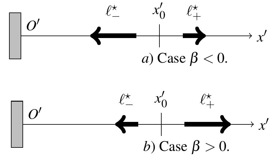
Figure 1: The two cases of the asymmetric persistent random walk in one dimension. a) The case $\beta<0$. In this case, $\ell_{-}>\ell_{+}$, the probability of passage at the origin $O^{\prime}$ is equal to $1$ and the average first-passage time is finite. b) The case $\beta>0$. In this case $\ell_{+}>\ell_{-}$, and the photon has a finite probability of never visiting the origin $O^{\prime}$.

5.1   An effective ”flip” process

As shown in the Reference (Rossetto, 2018), the Laplace transforms $\widehat{P}_{1}$ of the first-passage time distributions for $u_{0}=\pm 1$ are related by

$$\widehat{P}_{1}(s\,|\,x^{\prime}_{0},\,+1)=\widehat{P}_{1}(s\,|\,x^{\prime}_{0},\,-1)\widehat{f}(s),$$ (8)

$$\text{where }\widehat{f}(s)=\frac{(1-\beta)\gamma}{\frac{\ell}{c}s+\gamma+\sqrt{(\frac{\ell}{c}s+\gamma)^{2}-1}}.\quad$$ (9)

The equation (8) shows that the first-passage time process of a CTPRW with initial direction $u_{0}=+1$ is the convolution of the first-passage time process of a CTPRW with $u_{0}=-1$ with a new process $F$ that I call a ”flip process”.

A CTPRW with initial direction $u_{0}=+1$ has the following effective behavior: it first spends a certain time to ”flip” (that is: to set itself in the same initial conditions as a CTPRW process with $u_{0}=-1$) then it follows the course of a regular CTPRW with $u_{0}=-1$ until it reaches the origin. As $\widehat{f}$ is independent of $x^{\prime}_{0}$, the ”flip” is completely independent of the initial distance to the origin and its effect cannot be interpreted as, or reproduced by, a shift of the starting position $x^{\prime}_{0}$.

The photons emitted away from $O^{\prime}$ (with $u_{0}=+1$) are thus observed by the moving operator in $O^{\prime}$ with a random supplementary delay corresponding to the ”flip time”.

5.2   Statistics of the ”flip” process

The inverse Laplace transform of $\widehat{f}$ is the distribution of time until the ”flip” occurs. Using Reference (Abramowitz and Stegun, 1972, formulæ 29.3.52 and 29.3.53), one obtains from Equation (9)

$$f(t)=(1-\beta)\gamma\,\frac{\operatorname{\mathrm{I}}_{1}(ct/\ell)}{t}\mathrm{e}^{-\gamma ct/\ell}.$$ (10)

Up to my knowledge, this expression is not a referenced probability distribution. Note that $f(t)=P_{1}(t\,|\,0,+1)$ so that, when $x^{\prime}_{0}=0$, the ”flip” time is also the time of return at $O^{\prime}$. For $\beta<0$, the mean ”flip” time and its variance are

$$\mathbb{E}[F]=\frac{1}{|\beta|}\frac{\ell}{\gamma c},\qquad\operatorname{Var}(F)=\frac{1}{|\beta|^{3}}\left(\frac{\ell}{\gamma c}\right)^{2}.$$ (11)

More properties of $F$ are given in the Appendix B.

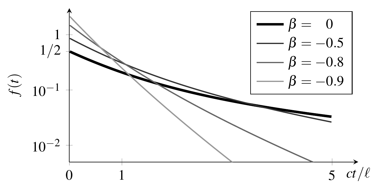
Figure 2: Graphs of the distribution of the ”flip” process for some values of $\beta\leq 0$. For $\beta=0$, the distribution is normalized, but it has no finite moments. As $\beta$ approaches $-1$, the time distribution gets more concentrated near $t=0$.

6   Lorentz covariance in two dimensions

As previously suggested in the case of the one-dimensional persistent random walk, relativistic random walks should be constructed as Markov processes in phase space. In two dimensions, a point in the photon’s phase space is a pair $(\mathbf{r},\,\hat{\mathbf{u}})$ where $\mathbf{r}$ is the two-dimensional position and $\hat{\mathbf{u}}$ is the two-dimensional unit vector of the direction of propagation. The exact solution of the two-dimensional CTPRW in the reference frame where the cloud of scatterers is at rest, $\mathcal{R}$, with initial conditions $\mathsf{X}_{0}=(\mathbf{r}_{0}=0,\,\hat{\mathbf{u}}_{0})$ at $t=0$ was recently published (Rossetto, 2017). It essentially depends on the Lorentz invariant $c^{2}t^{2}-\mathbf{r}^{2}$ and on the variable $\mathcal{X}$:

$$\mathcal{X}^{2}=\frac{2}{\ell^{2}}\frac{(ct-\mathbf{r}\cdot\hat{\mathbf{u}})(ct-\mathbf{r}\cdot\hat{\mathbf{u}}_{0})}{1-\hat{\mathbf{u}}\cdot\hat{\mathbf{u}}_{0}}-\xi^{2}$$ (12)

($\xi=\sqrt{c^{2}t^{2}-\mathbf{r}^{2}}/\ell$) and it decomposes as the sum $g=g_{0}+g_{1}+g_{\infty}$ where $g_{0}$ is the unscattered contribution (Dirac delta function), $g_{1}$ is the single scattering contribution and

$$g_{\infty}(t,\,\mathsf{X}\,|\,\mathsf{X}_{0})=\frac{1}{2\pi{\ell}^{2}}\frac{\mathrm{e}^{-ct/\ell}}{1-\hat{\mathbf{u}}\cdot\hat{\mathbf{u}}_{0}}\Theta(ct-\|\mathbf{r}\|)\times\dots{\\ }\cdots\operatorname{Re}\left[\operatorname{E_{1}}(\mathrm{i}\mathcal{X})\mathrm{e}^{\mathrm{i}\mathcal{X}}-\operatorname{E_{1}}\left(\mathrm{i}\mathcal{X}-\xi\right)\mathrm{e}^{\mathrm{i}\mathcal{X}}\right]$$

is the multiple scattering contribution, with $\operatorname{E_{1}}$ the exponential integral function (Abramowitz and Stegun, 1972, Chapter 5).

As the process is Markovian, Chapman-Kolmogorov’s relation is fulfilled and the expression (6) is valid using the convention that, in two dimensions, the phase space integral $\int_{\mathsf{X}}$ denotes $\int_{\mathbf{r}}\int_{\hat{\mathbf{u}}}$. Again, Chapman-Kolmogorov’s relation is satisfied for all pulse initial conditions in phase space separately, but not necessarily for their superpositions.

The velocity of $\mathcal{R}$ in $\mathcal{R}^{\prime}$ is denoted, without loss of generality, by $\mathbf{v}=v\hat{\mathbf{e}}_{x}$. The coordinates of $\mathbf{r}$ transform into the coordinates of $\mathbf{r}^{\prime}$ by a Lorentz boost whereas the coordinates of $\hat{\mathbf{u}}$ and $\hat{\mathbf{u}}_{0}$ transform according to the addition law of velocities. Using these relations and elementary algebra operations shows that the variable $\mathcal{X}$ is Lorentz invariant (see the Appendix for details). The Lorentz covariance of the term $g_{\infty}$ follows and that of the terms $g_{0}$ and $g_{1}$ is straightforward.

7   The Brownian limit

As mentioned in the introduction, the telegrapher’s equation also appears as a modification of Smoluchowski’s diffusion equation (Brinkman, 1956; Sack, 1956), which microscopic model is Brownian motion. The classical constructions of Brownian motion are, in various ways, mathematical limits of an underlying random walk performing small steps at a rate going to infinity (see for instance the works of Wiener (1923) and Itô (1950)). This limit implies that the instantaneous speed of a particule performing the random walk is infinite. Although the limit of infinite speed is legitimate in classical physics, it does not comply with special relativity. Arguably, a relativistic counterpart of the classical Brownian motion should involve particles moving at largest possible speed, the speed of light $c$. Such particles then must be massless. The relativistic Brownian motion of massive particles has been extensively studied by Dunkel and Hänggi (Dunkel and Hänggi, 2005a, b, 2009) using stochastic differential equations, where the limit of infinite rate pertains to the concept of noise.

The Brownian limit of the general solution (5) corresponds to taking the speed of light $c$ to infinity and the mean free path $\ell$ to zero, while keeping the product $\ell c=2D$ constant. It yields a Gaussian distribution in $\mathcal{R}^{\prime}$ centered at $\beta ct^{\prime}=vt^{\prime}$ and of variance $2Dt^{\prime}$. The contributions of the initial direction of propagation $u_{0}$ vanish in the Brownian limit of Equation (5). The two cases $u_{0}=\pm 1$ in the Equation (5a) are therefore undistinguishable such that the solution $g(x^{\prime},\,t^{\prime})$ in $\mathcal{R}^{\prime}$ is their sum. Lorentz invariance (and thus causality) also disappears in this limit.

In the limit $c\to\infty$, the Lorentz factor is $\gamma\simeq 1+\frac{1}{2}\beta^{2}$. The expansion $\xi\simeq\frac{ct}{\ell}-x^{2}/2ct\ell$ and the asymptotic form $\operatorname{\mathrm{I}}_{\nu}(x)\simeq\mathrm{e}^{x}/\sqrt{2\pi x}$ (Abramowitz and Stegun, 1972, formula 9.7.1) give

$$g(x^{\prime},\,t^{\prime})\simeq\frac{\exp\big{(}\frac{x^{\prime 2}}{4c^{2}t^{\prime 2}}\big{)}}{\sqrt{2\pi ct^{\prime}\ell}}\exp\left[-\frac{(x^{\prime}-\beta ct^{\prime})^{2}}{2\ell ct^{\prime}}\right]\Theta(ct^{\prime}-|x^{\prime}|).$$

The total solution is, in the limit $c\to\infty$ and $\ell\to 0$ with $c\ell=2D$ constant, equal to

$$g(x^{\prime},\,t^{\prime})=\frac{1}{\sqrt{4\pi Dt^{\prime}}}\exp\left[-\frac{(x^{\prime}-vt^{\prime})^{2}}{4Dt^{\prime}}\right].$$

8   Closing remarks

In this Letter, I have shown that the solutions of the radiative transfer equation are naturally Lorentz covariant and can be obtained from the solutions expressed in phase space. I proved that these solutions satisfy the transitivity of Green’s functions only in phase space, not in position space. In one dimension, I have unveiled a ”flip process” that translates as a delay in the measured signal for photons emitted away from the observer. I also have shown that the moments of a signal measured from a pulse become finite in the case where the observer is moving toward the source ($\beta<0$). These results have been obtained thanks to the stochastic model of continous-time persistent random walks (CTPRW), which are Markov processes in phase space. I showed that the Markov property of the CTPRW follows from the memorylessness of the exponential probability distribution and the phase space representation.

One should naturally expect that the same approach applies in three dimensions. The three-dimensional Green’s function would indeed be of interest in astrophysics and medical imaging, but no exact solutions are known in three dimensions, even for the energy density (the process in position space). It is however possible that a solution for the radiance, i. e. in phase space, exists. Such a solution could be expressed in terms of a Lorentz invariant variable such as $\mathcal{X}$ from Equation (12), which three-dimensional counterpart also is Lorentz invariant. In any event, I believe that this Letter will trigger progress in this direction.

Using the limit $c\to\infty$, I showed that the CTPRW is an extension of Brownian motion and therefore that radiative transfer is a natural extension of diffusion in special relativity, requiring a solution in phase space. Several works have already suggested to consider relativistic Brownian motion as a process in phase space (Dudley, 1966; Hakim, 1968). A straightforward extension of the CTPRW for massive particles would, for instance, be a process selecting a random momentum according the Jüttner-Maxwell distribution (Jüttner, 1911), and a random, exponentially distributed, free travel distance at each step. Such a construction could avoid the difficulties related to the interpretation of stochastic integrals in the abovementioned works.

Appendices

A   Lorentz invariance of $\mathcal{X}$

Here is a proof that the variable $\mathcal{X}$ defined by the Equation (12) is a relativistic invariant. In two dimensions, the space-time coordinates of $\mathbf{r}=(x,\,y)$ transform as

$$x=\gamma x^{\prime}-\beta\gamma ct^{\prime},\qquad y=y^{\prime},\qquad ct=\gamma ct^{\prime}-\beta\gamma x^{\prime},$$

whereas the components of the direction of propagation $\hat{\mathbf{u}}=(u_{x},\,u_{y})$ transform through the velocity addition law :

$$u_{x}=\frac{u^{\prime}_{x}-\beta}{1-\beta u^{\prime}_{x}},\qquad u_{y}=\frac{u^{\prime}_{y}}{\gamma(1-\beta u^{\prime}_{x})}.$$

Therefore we obtain

$$\begin{split}ct-\mathbf{r}\cdot\hat{\mathbf{u}}&=\gamma ct^{\prime}-\beta\gamma x^{\prime}-\frac{(\gamma x^{\prime}-\beta\gamma ct^{\prime})(u^{\prime}_{x}-\beta)+y^{\prime}u^{\prime}_{y}/\gamma}{1-\beta u^{\prime}_{x}}\\ &=\frac{ct^{\prime}-\mathbf{r}^{\prime}\cdot\hat{\mathbf{u}}^{\prime}}{\gamma(1-\beta u^{\prime}_{x})}.\end{split}$$

Moreover,

$$\hat{\mathbf{u}}\cdot\hat{\mathbf{u}}_{0}=\frac{u^{\prime}_{x}-\beta}{1-\beta u^{\prime}_{x}}\frac{u^{\prime}_{0x}-\beta}{1-\beta u^{\prime}_{0x}}+\frac{u^{\prime}_{y}}{\gamma(1-\beta u^{\prime}_{x})}\frac{u^{\prime}_{0y}}{\gamma(1-\beta u^{\prime}_{0x})},$$

and so

$$\begin{split}1-\hat{\mathbf{u}}\cdot\hat{\mathbf{u}}_{0}=\frac{1-\beta^{2}}{(1-\beta u^{\prime}_{x})(1-\beta u^{\prime}_{0x})}(1-\hat{\mathbf{u}}^{\prime}\cdot\hat{\mathbf{u}}^{\prime}_{0}).\end{split}$$

As a conclusion, the fraction in Eq. (12) transforms as

$$\frac{(ct-\mathbf{r}\cdot\hat{\mathbf{u}})(ct-\mathbf{r}\cdot\hat{\mathbf{u}}_{0})}{1-\hat{\mathbf{u}}\cdot\hat{\mathbf{u}}_{0}}=\frac{(ct^{\prime}-\mathbf{r}^{\prime}\cdot\hat{\mathbf{u}}^{\prime})(ct^{\prime}-\mathbf{r}^{\prime}\cdot\hat{\mathbf{u}}^{\prime}_{0})}{1-\hat{\mathbf{u}}^{\prime}\cdot\hat{\mathbf{u}}^{\prime}_{0}}.$$

This proves the announced invariance of $\mathcal{X}$.

B   More properties of $F$

The probability density of the ”flip” time is, to my knowledge, not a referenced probability density function. I give here the expressions of the probability density $\sigma_{n}$ of the sum of $n\geq 1$ independent ”flip” processes $F_{1}+F_{2}+\cdots+F_{n}=\Sigma_{n}$ and the moments of order $k$ of $\Sigma_{n}$. These are established using the relation $\sigma_{n}=f^{\otimes n}$ and its Laplace transform $\widehat{\sigma}_{n}=\big{(}\widehat{f}\big{)}^{n}$, where $\otimes$ denotes convolution and ${}_{2}F_{1}$ is Gauss’s hypergeometric function.

$$\sigma_{n}(t) = n\big{[}(1-\beta)\gamma\big{]}^{n}\;\frac{\operatorname{\mathrm{I}}_{n}(ct/\ell)}{t}\mathrm{e}^{-\gamma ct/\ell},$$ (13a)

$$\mathbb{E}\big{[}\Sigma_{n}^{k}\big{]} = \left(\frac{1-\beta}{2\gamma}\right)^{n}\,\left(\frac{\ell}{\gamma c}\right)^{k}\,\frac{(n+k-1)!}{(n-1)!}\dots$$ (13d)

$$\qquad\dots\;{}_{2}F_{1}\!\left(\begin{array}[]{c}\frac{n+k}{2}\;\frac{n+k+1}{2}\\ n+1\end{array}\;\vrule\;\frac{1}{\gamma^{2}}\right).$$

References

- Abramowitz and Stegun (1972) Milton Abramowitz and Irene A. Stegun (1972), Handbook of mathematical functions, 10th edition, Dover, New York.
- Asllanaj et al. (2014) Fatmir Asllanaj, Sylvain Contassot-Vivier, André Liemert and Alwin Kienle (2014), Radiative transfer equation for predicting light propagation in biological media: comparison of a modified finite volume method, the Monte Carlo technique, and an exact analytical solution, J. Biomed. Opt. 19, article 015002.
- Brinkman (1956) H. C. Brinkman (1956), Brownian motion in a field of force and the diffusion theory of chemical reactions, Physica 22, pages 29–34.
- Chandrasekhar (1960) Subrahmanyan Chandrasekhar (1960), Radiative transfer, Dover, New York.
- DeWitt-Morette and Foong (1989) Cécile DeWitt-Morette and S. K. Foong (1989), Path-integral solutions of wave equations with dissipation, Phys. Rev. Lett. 62, pages 2201–2204.
- Dudley (1966) R. M. Dudley (1966), Lorentz-invariant Markov process in relativistic phase space, Arkiv. Mat. 6, pages 241–268.
- Dunkel and Hänggi (2005a) Jörn Dunkel and Peter Hänggi (2005a), Theory of relativistic Brownian motion : The 1+1 dimensional case, Phys. Rev. E 71, article 016124.
- Dunkel and Hänggi (2005b) Jörn Dunkel and Peter Hänggi (2005b), Theory of relativistic Brownian motion : The 1+3 dimensional case, Phys. Rev. E 72, article 036106.
- Dunkel and Hänggi (2009) Jörn Dunkel and Peter Hänggi (2009), Relativistic Brownian motion, Phys. Rep. 471, pages 1–73.
- Foong (1992) See Kit Foong (1992), First-passage time maximum displacement and kac s solution of the telegrapher equation, Phys. Rev. A 46, pages R707–710.
- Foong and Kanno (1994) See Kit Foong and S. Kanno (1994), Properties of the telegrapher random process with or without a trap, Stoch. Proc. App. 53, pages 147–173.
- Fürth (1920) Reinhold Fürth (1920), Die Brownsche Bewegung bei Berücksichtigung einer Persistenz der Bewegungsrichtung mit Anwendungen auf die Bewegung lebender Infusorien, Zeit. Phys. 2, pages 244–256.
- Goldstein (1951) S. Goldstein (1951), On diffusion by discontinuous movements and on the telegraph equation, Q. J. Mech. Appl. Math. 4, pages 129–156.
- Hakim (1968) R. Hakim (1968), Relativistic stochastic processes, J. Math. Phys. 9, pages 1805–1818.
- Hemmer (1961) P. Chr. Hemmer (1961), On the generalization of Smoluchowski’s diffusion equation, Physica (Amsterdam) 27, pages 79–82.
- Ishimaru (1978) Akira Ishimaru (1978), Wave propagation and scattering in random media, Academic Press, New York.
- Itô (1950) Kiyosi Itô (1950), Brownian motions in a Lie group, Proc. Japan. Acad. 26, pages 4–10.
- Jakob et al. (2010) W. Jakob, A. Arbree, K. Moon, J. and Bala and S. Marschner (2010), A radiative transfer framework for rendering materials with anisotropic structure, ACM Transactions on Graphics 29, pages 1––13.
- Jüttner (1911) Ferencz Jüttner (1911), Das Maxwellsche Gesetz der Geschwindigkeitsverteilung in der Relativtheorie, Ann. Phys. 339, pages 856–882.
- Kac (1974) Mark Kac (1974), A stochastic model related to the telegrapher’s equation, Rocky Mountain J. Math. 4, pages 497–509.
- Majumdar (2005) Satya Majumdar (2005), The legacy of Albert Einstein, Current Science 89, pages 2076–2092.
- Marshak and Davis (2005) A. Marshak and A. B. Davis (2005), 3D radiative transfer in cloudy atmospheres, Springer, Berlin.
- Masoliver et al. (1989) Jaume Masoliver, Katja Lindenberg and George H. Weiss (1989), A continuous-time generalization of the persistent random walk, Physica. A 157, pages 891–898.
- Morse and Feshbach (1953) Philip Morse and Herman Feshbach (1953), Methods of theoretical physics 1, McGraw Hill, New York.
- Paasschens (1997) J. C. J. Paasschens (1997), Solution ot the time-dependent Boltzmann equation, Phys. Rev. E 56, pages 1135–1141.
- Rossetto (2013) Vincent Rossetto (2013), Local time in diffusive media and applications to imaging, Phys. Rev. E 88, article 022103.
- Rossetto (2017) Vincent Rossetto (2017), Space-time domain velocity distributions in isotropic radiative transfer in two dimensions, J. Phys. A: Math. Theor. 50, article 165001.
- Rossetto (2018) Vincent Rossetto (2018), The one-dimensional asymmetric persistent random walk, J. Stat. Mech. 2018, article 043204.
- Sack (1956) R. A. Sack (1956), A modification of Smoluchowski’s diffusion equation, Physica 22, pages 917–918.
- Sato (1993) Haruo Sato (1993), Energy transport in one- and two-dimensional scattering media: Analytic solutions of the multiple isotropic scattering model, Geo. Phys. J. Int. 117, pages 487–494.
- Shang and Gao (1988) T. Shang and L. Gao (1988), Transportation theory of multiple scattering and its application to seismic coda waves of impulse source, Scientia Sinica B 31, pages 1503–1514.
- Taylor (1922) G. I. Taylor (1922), Diffusion by continuous movements, Proc. London Math. Soc. 20(1), pages 196–212.
- Thomson (1855) William Thomson (1855), On the theory of the electric telegraph, Proc. R. Soc. Lond. 7, pages 382–399.
- Weiss (2002) George H. Weiss (2002), Some applications of persistent random walks and the telegrapher equation, Physica A 311, pages 381–410.
- Wiener (1923) Norbert Wiener (1923), Differential space, J. Math. Phys. 2, pages 131–174.