Taming the time evolution in overdamped systems: shortcuts elaborated from fast-forward and time-reversed protocols
Abstract
Using a reverse-engineering approach on the time-distorted solution in a reference potential, we work out the external driving potential to be applied to a Brownian system in order to slow or accelerate the dynamics, or even to invert the arrow of time. By welding a direct and time-reversed evolution towards a well chosen common intermediate state, we derive analytically a smooth protocol to connect two arbitrary states in an arbitrarily short amount of time. Not only does the reverse-engineering approach proposed in this Letter contain the current—rather limited—catalogue of explicit protocols but it also provides a systematic strategy to build the connection between arbitrary states with a physically admissible driving. Optimization and further generalizations are also discussed.
Shortcut To Adiabaticity techniques originally aim at reaching adiabatic outcomes in a finite amount of time [1]. Adiabatic should be understood here in its quantum sense, synonymous with “sufficiently slowly driven” 111And not in the thermodynamic sense of zero heat.. These methods have been extended to generate shortcuts between two states, regardless of the existence of an adiabatic connection between them [1]. While this field is rooted in quantum mechanics [3, 4], related questions emerge in other domains, namely classical mechanics [5, 6, 7, 8, 9, 10, 11] and stochastic thermodynamics [12, 13, 14, 15, 16, 11, 17, 18]. Yet, the question of transposing to statistical physics protocols originally developed in quantum mechanics is delicate. For instance, the so-called counterdiabatic protocol (also dubbed transitionless tracking) valid for any initial condition [19, 20] can be directly transposed to overdamped dynamics [13]. However, the very same procedure yields non conservative forcings, experimentally problematic to achieve, with underdamped systems [13, 1]. Among the set of tools for accelerating the dynamics, other classes of solutions propose tailor-made protocols based on the specifics of the initial and final states, both in quantum mechanics [21, 20, 7, 22, 23, 24, 25] and in statistical physics [26, 12, 27, 28]. More general optimal protocols in small thermodynamic systems have been obtained from a mapping to optimal transport, establishing an unexpected connection with cosmology but requiring a numerical resolution [29, 30, 31, 32, 33]. These protocols generically lead to discontinuous-in-time driving forces [26, 30], which raises a delicate experimental challenge for implementation.
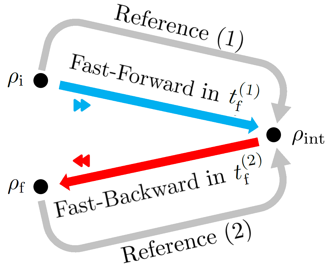
A central question is thus to work out shortcuts to transformations between arbitrary states, that should involve non-singular forces and be expressible in closed form. This is the question we solve in the present Letter, within the framework of the Fokker-Planck equation [34], which governs the evolution of the probability density of Brownian objects, with and denoting position and time. To this end, we proceed in two steps. First, we show how to distort and control a reference dynamics, i.e., the time evolution taking place in a reference external potential , with a well chosen external potential . The realization of such drivings is now achieved experimentally in a number of domains, from cold atom physics [35] to colloids [36], thanks to a proper steering of the optical potential applied to the system [16, 17, 37]. This will allow us to accelerate the reference dynamics (fast-forward) [21], or to decelerate it (slow-forward), and even to freeze the evolution. Interestingly, this also opens the way to reverse time’s arrow and devise a backward drive at arbitrary speed. Second, we combine a fast-forward drive towards a suitably chosen intermediate state with a fast-backward protocol from , to get a whole family of smooth shortcuts, as depicted in Fig. 1. In doing so, the system can be brought from a chosen state to another chosen state , in an arbitrary time. Both states can be equilibrium or, more generally, out-of-equilibrium [38, 39].
Reverse engineered potential.- The Brownian objects considered, such as colloids in dilute conditions, are immersed in a thermal bath at temperature and submitted to an external force field stemming from a potential . The Fokker-Planck equation for the probability density reads
| (1) |
where is the bath friction coefficient and , with the Boltzmann’s constant. A unique solution for can be obtained by imposing a prescribed time evolution for the density , from an initial to a final state 222For the moment, we focus our attention on single-step connections. The concept of the intermediate state will return when designing the welding strategy.. Once , together with the operating time , have been chosen, Eq. (1) is nothing but a first order differential equation for the external force that should be applied to the system to achieve the appropriate driving. Assuming that the density current vanishes at the boundaries of the system, , we get
| (2) |
Unfortunately, except in a few cases, like that of a Gaussian distribution [26, 12], shape preserving evolutions [41], or other very specific situations [41, 33], Eq. (2) is impractical since it does not lead to an explicit closed-form potential [42]. We thus seek an alternative route that provides a systematic approach to obtain admissible driving protocols in closed-form.
From Fast-Forward (FF) to Fast-Backward (FB).- The idea is to take advantage of the knowledge of a reference non-trivial dynamics for to distort its time evolution by finding the appropriate driving potential. First, we show how a time contraction can be performed to force the system to reach equilibrium in a finite amount of time. Such a FF protocol realizes in finite time a process that takes an infinite amount of time, when the system is unperturbed. Beyond FF, FB protocols—and also slow forward or backward ones—can also be engineered. We subsequently explain under which conditions the driving force remains continuous for all times, a key requirement for practical implementation.
Consider a reference process, i.e., a known solution of the Fokker-Planck equation (1) in a confinement potential over a time interval , which we write as a continuity equation
| (3a) | ||||
| (3b) | ||||
We define the desired prescribed density as
| (4) |
through a time manipulation of the reference process, embedded in the function . The prescribed and the reference evolution go through the same states, but displayed at a different frame rate and/or time ordering. Indeed, depending on the choice for , one can play “the movie” at FF speed (), at slow motion (), pause it (), or even rewind it: either at slow backward motion () or at FB speed (). In the latter case, , our procedure enables a new possibility: the design of a potential to invert time’s arrow for an irreversible evolution obeying the Fokker-Planck equation.
Introducing Eqs. (3) and (4) into Eq. (2), and defining , which measures the departure from the reference potential, we get
| (5) |
where the time dependence of the protocol is encapsulated in and its derivative . For simplicity, we restrict ourselves to that are monotonic functions of time, either of FF ( and ) or of FB ( and ) type. The times and can be finite or infinite. Of particular relevance for experimental applications though is the shortcut of an infinite process (infinite but finite ), e.g., for building irreversible nano heat engines [43, 44, 45, 46, 47, 48, 28, 49, 50].
For the sake of simplicity, we consider hereafter a static reference potential . Such a potential is convenient; it makes it possible to analytically obtain through an expansion in eigenmodes, as shown below 333Yet, Eq. (5) remains valid for a time-dependent reference potential, should this choice be more appropriate for a specific situation. With , the reference process is thus the relaxation to the equilibrium distribution for : . In order to accelerate such an everlasting dynamics, we impose . For our purposes, it is adequate to use the family of functions
| (6) |
where is a characteristic time. The divergence of at implies that , which suggests that may diverge at the final time. However, the velocity field vanishes at and thus the behavior of needs to be elucidated.
Regularity of the driving potential.- The family defined in Eq. (6) has the property . This guarantees the continuity of the force at the initial time, as implied by Eq. (5). We show now on general grounds that the force field remains continuous even at , provided the reference potential is confining—in the sense that there exists a well-defined equilibrium density. The proof uses the expansion in eigenmodes for the solution of the reference process, and a mapping to a quantum problem. Introducing leads to the time-dependent Schrödinger equation with Hamiltonian [52],
| (7) |
The smallest eigenvalue, associated to the equilibrium distribution, is zero: . The other eigenvalues of are positive, , implying that the corresponding modes decay exponentially in time. Specifically, , where is the eigenfunction associated to the -th eigenvalue 444The eigenfunctions are mutually orthogonal and normalized, , where denotes the integration domain..
The expansion of the reference process in the eigenbasis reads
| (8) |
where is the partition function and . We are interested in the limit , for which . From Eq. (8) we deduce
| (9) |
where and . As a result, to the lowest order in , we get
| (10) |
which combined with Eq. (5) gives
| (11) |
There is a vast set of diverging functions including the family (6) that forces the cancellation of the right hand side of Eq. (11) when approaches [42], a requirement that implies that the driving force remains continuous at the final time. In our proof, the existence of a well-defined partition function is important. This is not the case for a free expansion, , in an infinite or semi-infinite space [42]. However, the argument remains valid for a reference free diffusing system within a finite box, as shown below.
To sum up, Eq. (5) provides the smooth potential needed to tune at will the reference process according to the time mapping function . Despite the limited number of analytically solvable reference processes [42], we can always rely on an expansion as in Eq. (8), but with a certain cutoff—examples are provided below. In doing so, the tailored process does not strictly reach the target state, but its distance thereto—e.g., with the norm—can be made as small as desired [42, 54].
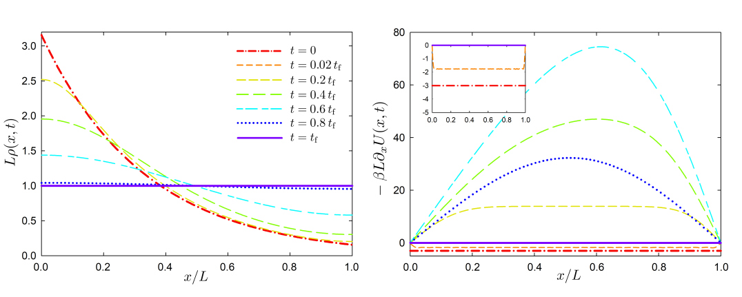
Diffusion in a box.- We illustrate the time manipulation procedure with the FF transformation of the free diffusion for a dilute gas within a finite box, . The gas is initially at equilibrium in the presence of a constant and homogeneous force, , with thus a sedimentation profile. In the reference process, at time , the force is suddenly removed and it takes an infinite time to reach the stationary homogeneous state. The time scale of the relaxation is characterized by .
We have chosen from Eq. (6) with , , and . The results for the FF transformation are displayed in Fig. 2, for the density of the gas and the force . Apart from a short time window where the forces are negative because of continuity, the forces required to accelerate homogenization are positive, pushing the system in the direction opposite to that of the initial force. As highlighted above, the protocol is smooth in time, including the initial and final times. In general, faster accelerations have a higher cost. Both the magnitude of the required force and the excess irreversible work increase as is decreased [42].
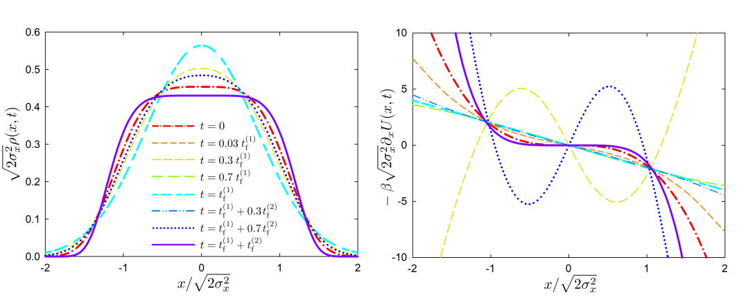
Connecting arbitrary states.- We come back to the welding idea conveyed in Fig. 1. For the sake of concreteness, the initial and final densities are the equilibrium distributions corresponding, respectively, to the initial and final potential and . None of these two potentials provides a convenient reference potential: the associated reference dynamics cannot be analytically solved and the FF idea results inoperative. Here, the welding method offers a solution. Indeed, choosing a Gaussian intermediate state () is free of the above difficulties, and solvable. We thus take , where stands for the variance of [42]. As previously, we accelerate the forward (FF) and backward (FB) processes by a factor ten, , with . For both the FF and FB steps, the function is taken to be the same, with 555To account for time reversal and the time shift in the FB part, .. The results for the welded FF and FB protocols are displayed in Fig. 3. In the first step, the tails of the density have to be pushed away from the center and the confinement needs to be strengthened in the central region to reach faster ; hence the -shape force. During the second stage, the requirements are opposite, leading to an inverted -shape. The force protocol is continuous for all times, including the initial and final times for both steps of the welding strategy.
We have focused on a specific functional shape for the time manipulation, Eq. (6), in order to ensure the continuity properties that we desire for the protocol. One may consider optimization problems, such as finding the time manipulation that minimizes some relevant observable—like the excess irreversible work [29, 30, 31, 32, 33]. Remarkably, it is possible to show that such an optimization over all FF protocols (attached to a given but with an arbitrary ) lead to processes delivering excess work at constant rate, as it happens with the full optimization [42]. Besides, when it comes to connecting two Gaussian states, the optimal FF protocol coincides with the full, unconstrained, optimum—and the minimum restricted to the specific family in Eq. (6) lies only 4% above it, for a ten-fold expansion of the state [42].
To sum up, we have developed a reverse-engineering technique in order to manipulate at will the time evolution of a reference process. This provides us with the external potential required to reach a target distribution in a desired time. Interestingly, not only does the framework allow for the acceleration of forward processes but also for the inversion of time’s arrow. Taking these time manipulated reference processes as building blocks, we have put forward a neat welding procedure to connect two arbitrary states in an arbitrarily small finite time. The method relies on a non-linear time mapping of two relaxation processes in the same harmonic potential; it produces by construction a smooth driving potential, with continuous force field, for all times. Finally, our procedure can be generalized to higher dimensional problems[56, 42]. Some possible venues for developments lie in the thermalization processes to build irreversible nano heat engines [43, 44, 45, 46, 47, 12, 28, 49, 50] or the genetic control of an evolving population [57, 58].
Acknowledgements.
We would like to thank S. Ciliberto, S. Dago and L. Bellon for fruitful discussions. This work was supported by the Agence Nationale de la Recherche research funding Grant No. ANR-18-CE30-0013, and project PGC2018-093998-B-I00 funded by FEDER/Ministerio de Ciencia e Innovación–Agencia Estatal de Investigación (Spain). C.A.P. also acknowledges financial support from Junta de Andalucía and European Social Fund through the program PAIDI-DOCTOR.References
- Guéry-Odelin et al. [2019] D. Guéry-Odelin, A. Ruschhaupt, A. Kiely, E. Torrontegui, S. Martínez-Garaot, and J. G. Muga, Shortcuts to adiabaticity: Concepts, methods, and applications, Rev. Mod. Phys. 91, 045001 (2019).
- Note [1] And not in the thermodynamic sense of zero heat.
- Chen et al. [2010a] X. Chen, A. Ruschhaupt, S. Schmidt, A. del Campo, D. Guéry-Odelin, and J. G. Muga, Fast optimal frictionless atom cooling in harmonic traps: Shortcut to adiabaticity, Phys. Rev. Lett. 104, 063002 (2010a).
- Chen et al. [2010b] X. Chen, I. Lizuain, A. Ruschhaupt, D. Guéry-Odelin, and J. G. Muga, Shortcut to adiabatic passage in two- and three-level atoms, Phys. Rev. Lett. 105, 123003 (2010b).
- Jarzynski [2013] C. Jarzynski, Generating shortcuts to adiabaticity in quantum and classical dynamics, Phys. Rev. A 88, 040101 (2013).
- Deng et al. [2013] J. Deng, Q.-h. Wang, Z. Liu, P. Hänggi, and J. Gong, Boosting work characteristics and overall heat-engine performance via shortcuts to adiabaticity: Quantum and classical systems, Phys. Rev. E 88, 062122 (2013).
- Guéry-Odelin and Muga [2014] D. Guéry-Odelin and J. G. Muga, Transport in a harmonic trap: Shortcuts to adiabaticity and robust protocols, Phys. Rev. A 90, 063425 (2014).
- Deffner et al. [2014] S. Deffner, C. Jarzynski, and A. del Campo, Classical and quantum shortcuts to adiabaticity for scale-invariant driving, Phys. Rev. X 4, 021013 (2014).
- Kolodrubetz et al. [2017] M. Kolodrubetz, D. Sels, P. Mehta, and A. Polkovnikov, Geometry and non-adiabatic response in quantum and classical systems, Physics Reports 697, 1 (2017).
- González-Resines et al. [2017] S. González-Resines, D. Guéry-Odelin, A. Tobalina, I. Lizuain, E. Torrontegui, and J. G. Muga, Invariant-based inverse engineering of crane control parameters, Phys. Rev. Applied 8, 054008 (2017).
- Patra and Jarzynski [2017] A. Patra and C. Jarzynski, Shortcuts to adiabaticity using flow fields, New Journal of Physics 19, 125009 (2017).
- Martínez et al. [2016a] I. A. Martínez, A. Petrosyan, D. Guéry-Odelin, E. Trizac, and S. Ciliberto, Engineered swift equilibration of a Brownian particle, Nature Physics 12, 843 (2016a).
- Li et al. [2017] G. Li, H. T. Quan, and Z. C. Tu, Shortcuts to isothermality and nonequilibrium work relations, Phys. Rev. E 96, 012144 (2017).
- Martínez et al. [2017] I. A. Martínez, E. Roldán, L. Dinis, and R. A. Rica, Colloidal heat engines: a review, Soft Matter 13, 22 (2017).
- Chupeau et al. [2018a] M. Chupeau, B. Besga, D. Guéry-Odelin, E. Trizac, A. Petrosyan, and S. Ciliberto, Thermal bath engineering for swift equilibration, Phys. Rev. E 98, 010104 (2018a).
- Ricci et al. [2017] F. Ricci, R. A. Rica, M. Spasenović, J. Gieseler, L. Rondin, L. Novotny, and R. Quidant, Optically levitated nanoparticle as a model system for stochastic bistable dynamics, Nature Communications 8, 15141 (2017).
- Dago et al. [2020] S. Dago, B. Besga, R. Mothe, D. Guéry-Odelin, E. Trizac, A. Petrosyan, L. Bellon, and S. Ciliberto, Engineered Swift Equilibration of Brownian particles: consequences of hydrodynamic coupling, SciPost Phys. 9, 64 (2020).
- Funo et al. [2020] K. Funo, N. Lambert, F. Nori, and C. Flindt, Shortcuts to adiabatic pumping in classical stochastic systems, Phys. Rev. Lett. 124, 150603 (2020).
- Demirplak and Rice [2003] M. Demirplak and S. A. Rice, Adiabatic population transfer with control fields, The Journal of Physical Chemistry A 107, 9937 (2003).
- Berry [2009] M. Berry, Transitionless quantum driving, Journal of Physics A 42, 365303 (2009).
- Masuda and Nakamura [2008] S. Masuda and K. Nakamura, Fast-forward problem in quantum mechanics, Phys. Rev. A 78, 062108 (2008).
- Vitanov and Shore [2015] N. V. Vitanov and B. W. Shore, Designer evolution of quantum systems by inverse engineering, Journal of Physics B 48, 12 (2015).
- Martínez-Garaot et al. [2016] S. Martínez-Garaot, M. Palmero, J. G. Muga, and D. Guéry-Odelin, Fast driving between arbitrary states of a quantum particle by trap deformation, Phys. Rev. A 94, 063418 (2016).
- Kang et al. [2016] Y.-H. Kang, Y.-H. Chen, Q.-C. Wu, B.-H. Huang, Y. Xia, and J. Song, Reverse engineering of a Hamiltonian by designing the evolution operators, Scientific Reports 6, 30151 (2016).
- Zhang et al. [2017] Q. Zhang, X. Chen, and D. Guéry-Odelin, Reverse engineering protocols for controlling spin dynamics, Scientific Reports 7, 15814 (2017).
- Schmiedl and Seifert [2007] T. Schmiedl and U. Seifert, Optimal finite-time processes in stochastic thermodynamics, Phys. Rev. Lett. 98, 108301 (2007).
- Chupeau et al. [2018b] M. Chupeau, S. Ciliberto, D. Guéry-Odelin, and E. Trizac, Engineered swift equilibration for Brownian objects: from underdamped to overdamped dynamics, New Journal of Physics 20, 075003 (2018b).
- Nakamura et al. [2020] K. Nakamura, J. Matrasulov, and Y. Izumida, Fast-forward approach to stochastic heat engine, Phys. Rev. E 102, 012129 (2020).
- Aurell et al. [2011] E. Aurell, C. Mejía-Monasterio, and P. Muratore-Ginanneschi, Optimal protocols and optimal transport in stochastic thermodynamics, Phys. Rev. Lett. 106, 250601 (2011).
- Aurell et al. [2012a] E. Aurell, C. Mejía-Monasterio, and P. Muratore-Ginanneschi, Boundary layers in stochastic thermodynamics, Phys. Rev. E 85, 020103 (2012a).
- Aurell et al. [2012b] E. Aurell, K. Gawȩdzki, C. Mejía-Monasterio, R. Mohayaee, and P. Muratore-Ginanneschi, Refined second law of thermodynamics for fast random processes, Journal of Statistical Physics 147, 487 (2012b).
- Muratore-Ginanneschi and Schwieger [2017] P. Muratore-Ginanneschi and K. Schwieger, An application of pontryagin’s principle to Brownian particle engineered equilibration, Entropy 19, 379 (2017).
- Zhang [2019] Y. Zhang, Work needed to drive a thermodynamic system between two distributions, EPL (Europhysics Letters) 128, 30002 (2019).
- Risken and Frank [1996] H. Risken and T. Frank, The Fokker-Planck Equation: Methods of Solution and Applications, Springer Series in Synergetics (Springer Berlin Heidelberg, 1996).
- Cohen-Tannoudji and Guéry-Odelin [2011] C. Cohen-Tannoudji and D. Guéry-Odelin, Advances in Atomic Physics: An Overview (World Scientific, 2011).
- Ciliberto [2017] S. Ciliberto, Experiments in stochastic thermodynamics: Short history and perspectives, Phys. Rev. X 7, 021051 (2017).
- Albay et al. [2020] J. A. C. Albay, C. Kwon, P.-Y. Lai, and Y. Jun, Work relation in instantaneous-equilibrium transition of forward and reverse processes, New Journal of Physics 22, 123049 (2020).
- Baldassarri et al. [2020] A. Baldassarri, A. Puglisi, and L. Sesta, Engineered swift equilibration of a Brownian gyrator, Phys. Rev. E 102, 030105 (2020).
- Prados [2021] A. Prados, Optimizing the relaxation route with optimal control, Phys. Rev. Research 3, 023128 (2021).
- Note [2] For the moment, we focus our attention on single-step connections. The concept of the intermediate state will return when designing the welding strategy.
- Zhang [2020] Y. Zhang, Optimization of stochastic thermodynamic machines, Journal of Statistical Physics 178, 1336 (2020).
- [42] See the Supplemental Material at xxxx for a discussion of shape-preserving dynamics (which includes a number of previously proposed explicit protocols) along with other simple proposals, the analysis of the continuity property of the steering potential, the dependence of the force intensity on the duration of the process, the study of optimal properties, the spectral decomposition backing up the welding procedure, the convergence of the resulting expansion, and the generalization to higher dimensions. A mathematica notebook solving the welding problem is also provided.
- Schmiedl and Seifert [2008] T. Schmiedl and U. Seifert, Efficiency at maximum power: An analytically solvable model for stochastic heat engines, EPL (Europhysics Letters) 81, 20003 (2008).
- Bo and Celani [2013] S. Bo and A. Celani, Entropic anomaly and maximal efficiency of microscopic heat engines, Phys. Rev. E 87, 050102 (2013).
- Tu [2014] Z. C. Tu, Stochastic heat engine with the consideration of inertial effects and shortcuts to adiabaticity, Phys. Rev. E 89, 052148 (2014).
- Martínez et al. [2015] I. A. Martínez, E. Roldán, L. Dinis, D. Petrov, and R. A. Rica, Adiabatic processes realized with a trapped brownian particle, Phys. Rev. Lett. 114, 120601 (2015).
- Dechant et al. [2015] A. Dechant, N. Kiesel, and E. Lutz, All-optical nanomechanical heat engine, Phys. Rev. Lett. 114, 183602 (2015).
- Martínez et al. [2016b] I. A. Martínez, E. Roldán, L. Dinis, D. Petrov, J. M. R. Parrondo, and R. A. Rica, Brownian carnot engine, Nature Physics 12, 67 (2016b).
- Plata et al. [2020] C. A. Plata, D. Guéry-Odelin, E. Trizac, and A. Prados, Building an irreversible carnot-like heat engine with an overdamped harmonic oscillator, Journal of Statistical Mechanics: Theory and Experiment , 093207 (2020).
- Tu [2020] Z.-C. Tu, Abstract models for heat engines, Frontiers of Physics 16, 33202 (2020).
- Note [3] Yet, Eq. (5\@@italiccorr) remains valid for a time-dependent reference potential, should this choice be more appropriate for a specific situation.
- [52] The advantage of this formulation lies in the use of the usual definition of scalar product in Hilbert space, with a weight function equal to unity. Equivalently, the Fokker-Planck operator can also be made Hermitian by introducing a scalar product with weight function .
- Note [4] The eigenfunctions are mutually orthogonal and normalized, , where denotes the integration domain.
- Carslaw [1950] H. S. Carslaw, Introduction to the theory of Fourier’s series and integrals (Dover Publications, New York, 1950).
- Note [5] To account for time reversal and the time shift in the FB part, .
- Frim et al. [2021] A. G. Frim, A. Zhong, S.-F. Chen, D. Mandal, and M. R. DeWeese, Engineered swift equilibration for arbitrary geometries, Phys. Rev. E 103, L030102 (2021).
- Iram et al. [2021] S. Iram, E. Dolson, J. Chiel, J. Pelesko, N. Krishnan, O. Güngör, B. Kuznets-Speck, S. Deffner, E. Ilker, J. G. Scott, and M. Hinczewski, Controlling the speed and trajectory of evolution with counterdiabatic driving, Nature Physics 17, 135 (2021).
- Weinreich [2021] D. M. Weinreich, Herding an evolving biological population with quantum control tools, Nature Physics 17, 17 (2021).