Interaction-induced wavefunction collapse

Abstract

Almost a century after the development of quantum mechanics, we still do not have a consensus on the process of collapse of wavefunctions. Some theories require the intervention of a conscious observer while some see it as a stochastic process, and most theories violate energy conservation. In this paper we hypothesise that the collapse of wavefunctions can be caused by interactions with other objects (macroscopic or microscopic) and energy is conserved in that process. To test various hypotheses regarding collapse of wavefunctions, we propose a model system which is the quantum analogue of a classical soft-impact oscillator. We propose some alternative postulates regarding the conditions for and the result of a collapse, and obtain the implication of each on the behavior of observable quantities, which can possibly be experimentally tested.

1 Introduction

Even though the theoretical structure of quantum mechanics is almost a century old, we have very little understanding of an important component of that theoretical structure—the collapse of the wavefunction. This concept is invoked to explain the results of experiments like the double-slit experiment. But it is largely ignored (or not needed) in most successful applications of quantum mechanics [16, 13].

The mainstream Copenhagen interpretation of quantum mechanics claims that, whenever an observation is made, the wavefunction of a quantum system collapses instantly to an eigenstate of the observable being measured. Many questions have been raised [7] regarding what constitutes an observation. “It would seem that the theory is exclusively concerned about ‘results of measurement’, and has nothing to say about anything else” wrote John Bell [4]. “What exactly qualifies some physical systems to play the role of ‘measurer’? Was the wavefunction of the world waiting to jump for thousands of millions of years until a single-celled living creature appeared? Or did it have to wait a little longer, for some better qualified system $\cdots$ with a PhD?” These questions have remained largely unanswered, and are considered to belong to the domain of philosophy rather than physics.

The founders of quantum mechanics did not provide an explicit mechanism for the collapse of the wavefunction and later it was termed as the measurement problem. Einstein believed that a complete description of physical reality would not be possible in this theory [9]. The famous Einstein-Podolsky-Rosen gedankenexperiment [10] illuminated the non-local structure of quantum entanglement and used it as an objection against the completeness of quantum mechanics. Einstein’s convictions about the determinism of nature inspired hidden variable theories which tried to rid quantum mechanics of indeterminacy. John Bell [5] showed that local hidden variable theories are incompatible with the predictions of quantum mechanics. Since then there have been several attempts to develop theories that incorporate a mechanism for wavefunction collapse.

Some have advocated for decoherence [20, 28] as a means to solve the measurement problem [26]. Even though it explains the absence of macroscopic superposition and the emergence of the classical world, it remains doubtful whether it has solved the measurement problem—as the founders of decoherence theory admit in their seminal papers [1, 19].

Dynamical collapse theories [3], on the other hand, supplant the unitary evolution with stochasticity and nonlinearity in such a way that all predictions of quantum mechanics are approximately reproduced in the microscopic limit while precluding macroscopic superpositions like Schrödinger cat states. A variety of collapse models have been developed that differ in their localization basis: while [23, 6] and [2] use the energy, momentum and spin basis respectively, the Ghirardi-Rimini-Weber (GRW) [11] and the Continuous Spontaneous Localisation (CSL)[12] operate in the position basis. The GRW model postulates wavefunction collapse as a random and spontaneous process. The collapsed wavefunction has a Gaussian form which is in turn dependent on certain natural constants that the theory introduces. Similar to it is the CSL model, the only difference being that the wavefunction in CSL collapses continuously in time [24]. This was followed by the Diosi-Penrose model [25] which is based on The Quantum Mechanics With Universal Position Localisation (QMUPL) [8] where gravity is responsible for the collapse of a wavefunction. These models are also characterized by the noise they use for generating the stochasticity they need to exhibit collapse.

John Bell had argued in favour of seeing the collapse of wavefunction as a natural process: “If the theory is to apply to anything but highly idealised laboratory operations, are we not obliged to admit that more or less ‘measurement-like’ processes are going on more or less all the time, more or less everywhere? Do we not have jumping then all the time?” [4]

In this paper, we hypothesise that collapse of a wavefunction does not require the intervention of a conscious observer. An interaction with another physical object—macroscopic or microscopic—can also cause the collapse of a wavefunction in the position space. The probability of occurrence of such an interaction depends on the overlap between their probability density functions.

If collapse-like processes indeed abound, as they reasonably should, the violation in energy conservation should be quite observable. The absence of such observations makes us hypothesise that any valid collapse mechanism must satisfy energy conservation, at least on average.

In order for a collapse model to be admissible, one has to propose postulates which have experimentally testable predictions. In this paper, we propose a model which can be used to test such postulates about interaction-induced wavefunction collapse, and work out the predictions of the various possible postulates when applied to that system.

2 The model system

Fig. 1 shows the classical analog of the system under consideration—a simple harmonic oscillator with mass $m$ and spring constant $k_{1}$ which can impact with a massless wall, cushioned by a spring of constant $k_{2}$. The variable $x$ is measured from the equilibrium position of the mass, and the wall is at $x_{\rm wall}$ when the spring $k_{2}$ is relaxed.

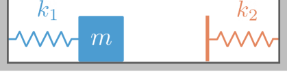
Figure 1: The classical soft-impact oscillator.

The classical system, with the inclusion of damping and external forcing, is known to exhibit a rich variety of dynamical phenomena which are initiated when the mass grazes the wall [27, 18]. We choose this particular system as the wall may be modeled either classically or quantum mechanically. This allows us to investigate the collapse of the wavefunction due to interaction with either a macroscopic or microscopic system.

The quantum version of the above system will be a particle in a potential well, which is the same as the harmonic oscillator potential for $x\leq x_{\rm wall}$ and is given by a different parabolic function for $x\geq x_{\rm wall}$. The potential function of the system is given by

$$V(x)=\left\{\begin{array}[]{ll}\frac{1}{2}k_{1}x^{2},&x\leq x_{\rm wall}\\ \frac{1}{2}k_{1}x^{2}+\frac{1}{2}k_{2}(x-x_{\rm wall})^{2},&x\geq x_{\rm wall}\end{array}\right.$$ (1)

We numerically solve the time-dependent Schrödinger equation for this system using the finite difference method by dividing the range $[-30,30]$ of the one-dimensional configuration space into 1,500 segments. We start from an initial wavefunction, which is a Gaussian function centered at $x=-5.0$, and standard deviation 1.0. This initial state corresponds, in the classical picture, to releasing the mass from the point $x=-5.0$, which would subsequently graze the wall located at $x=5.0$. The other parameters are taken as $m=1$, $k_{1}=1$, $k_{2}=10$. All quantities in this work are in units where $\hbar=1$. Fig. 2 shows snapshots of the dynamics of the wavefunction for this system.

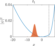
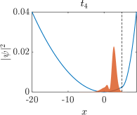
Figure 2: Evolution of the probability density distribution of the quantum particle at four time instants, with $t_{1}<t_{2}<t_{3}<t_{4}$. Dashed line indicates the equilibrium position of the wall. The potential function, plotted in blue for the sake of visualization, is not to scale.

To investigate the dynamics in the phase space, we compute the Wigner function

$$W(x,p)=\frac{1}{{\pi}\hbar}\int_{-\infty}^{\infty}\psi^{*}(x+y)\psi(x-y)e^{\frac{2ipy}{\hbar}}\,dy$$ (2)

which gives a real valued function of the position and momentum, which varies with time. Fig. 3 shows the plots of the Wigner function in the $x$–$p$ phase space at four different time instants. Prolonged observation of both $|\Psi^{2}|$ and the Wigner function shows that the time-evolution of the system is aperiodic.

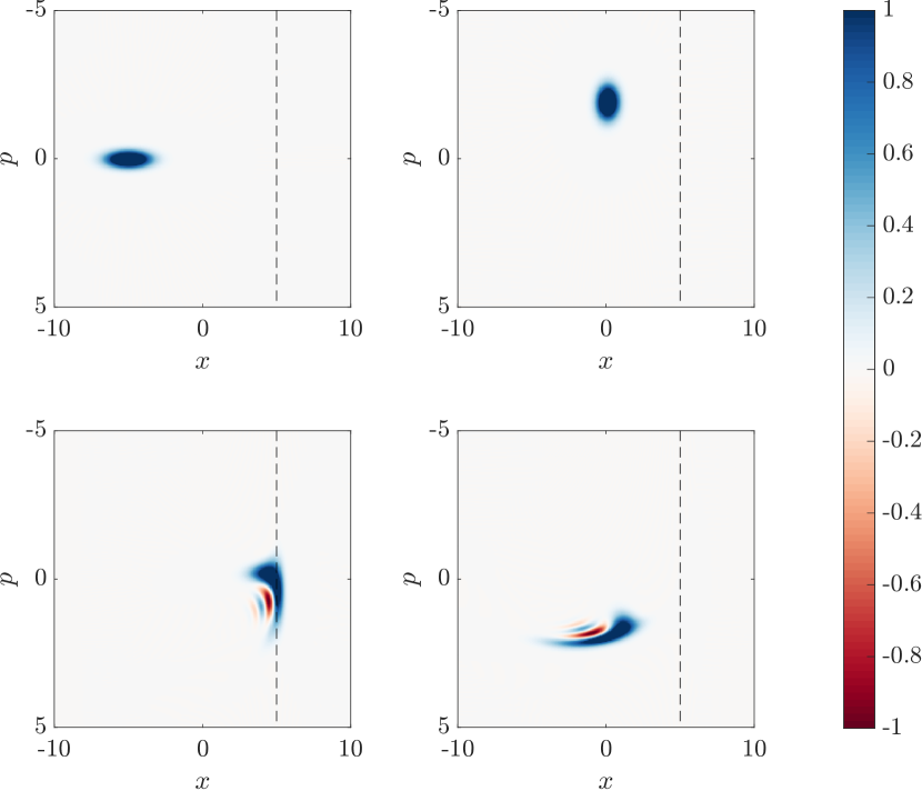
Figure 3: The evolution of the Wigner function at four time instants. The dashed line indicates the equilibrium position of the wall

Although all information about the system is contained in the wavefunction, or equivalently the Wigner quasiprobability distribution, it is hard to characterize the type of dynamics using them. A time series of real values is much more amenable to such analysis. Other investigators have used the expectation value of an observable for this purpose [22, 17, 21]. Since different states can have the same expectation value for an observable, we have used a different quantity, the absolute value of the overlap of the wavefunction at time $t$ with the initial wavefunction, given as

$$\mathcal{O}(t)=\langle\psi(0)|\psi(t)\rangle.$$

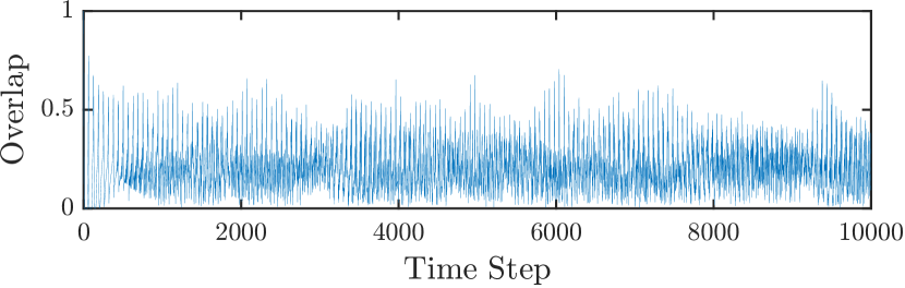
Figure 4: Plot of the overlap time series.

We find that, when the wall is placed far away from the particle, the behavior is periodic, like that of a harmonic oscillator. But when it comes closer (even when the classical system would not make any impact with the wall) the evolution of the wavefunction becomes aperiodic. Fig. 4 shows the time series of $\mathcal{O}(t)$ for a wall position corresponding to the classical grazing condition. We have performed the 0–1 test for chaos  [15], and have found that the behavior is not chaotic. A Fourier transform (Fig. 5) reveals that there are many discrete frequencies in its dynamics.

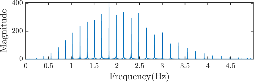
Figure 5: Frequency spectrum of the overlap time series.

Therefore, we conclude that, if the wavefunction is allowed to evolve indefinitely following the Schrödinger equation, the evolution of the wavefunction would be aperiodic, but is not chaotic as there is no sensitive dependence on initial condition. Moreover, the frequency spectrum does not have a continuum of frequencies and is a combination of a countable infinity of discrete frequencies.

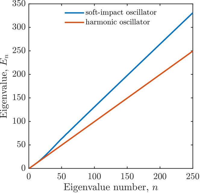
Figure 6: A plot of the first 250 eigenvalues.

A plot of the eigenvalues (Fig. 6) shows that for low values of $n$, the eigenvalues coincide with those of the harmonic oscillator. But for larger values of $n$, the graph has a different slope because eigenfunctions corresponding to large eigenvalues, which would usually be spread over a large region, cannot extend far beyond the position of the wall. An energy measurement can yield any of these eigenvalues and the expectation value is computed to be 13.125 GeV for our choice of initial state.

3 Collapse!

In the last section we considered a situation where the wavefunction evolves solely following the Schrödinger equation. In this section we bring in a new possibility. Since the wall can be considered to be a macroscopic object, an interaction of the particle with the wall (classically, an impact) may amount to a position measurement, which will cause the wavefunction to collapse. Following a collapse, the wavefunction will continue to evolve according to the Schrödinger equation until the next collapse. Thus, if this possibility is considered, the evolution would contain unitary evolution as well as non-unitary collapse processes.

Unlike the classical impact oscillator, the impact of the particle with the wall will be a probabilistic event, guided by the pre-collapse wavefunction of the particle. However, the present knowledge does not allow us to pinpoint a unique algorithm with which the instant of collapse and the location of the collapsed wavefunction can be simulated. So we posit different postulates regarding the mechanism of collapse, and work out the implication of each.

Postulate 1:

If the probability of finding the particle beyond the position of the wall exceeds a fraction $r$, i.e., if

$$\int_{x_{\rm wall}}^{\infty}|\Psi|^{2}dx\geq r,\;\;\;\;\;\;r\in(0,1)$$ (3)

then the wavefunction collapses to the position of the wall.

Postulate 2:

The same as Postulate 1, except that the number $r$ is not fixed, and is a random number between 0 and 1.

Postulate 3:

The same as Postulate 1, except that the wavefunction collapses to a point given by the pre-collapse probability distribution.

Postulate 4:

The same as Postulate 2, except that the wavefunction collapses to a point given by the pre-collapse probability distribution.

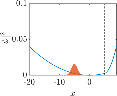
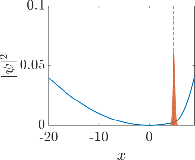
(a)                                                                (b)

Figure 7: (a) Initial Gaussian with mean $-5.0$ and SD=1, (b) the post-collapse wavefunction—a narrow Gaussian located at the position of the wall $x=5.0$ and SD=0.25. The potential function is shown in blue (not to scale).

In the following simulations, the initial wavefunction is considered to be a Gaussian function centred at $x=-5.0$ with standard deviation 1. The wall is placed at $x=5.0$, i.e., where the classical oscillator would experience grazing. For the first and third postulates, the value of $r$ is taken as 0.5. The post-collapse wavefunction is supposed to be an eigenfunction of the position operator, i.e., a delta function. However, the numerical routine would not work with such discontinuous functions. So we consider the post-collapse wavefunction to be a narrow Gaussian function of standard deviation 0.25 (Fig. 7). The parameter values are taken as: mass of the quantum particle $m=1$, spring constant of the spring attached to the mass $k_{1}=1$, the spring constant corresponding to the soft wall $k_{2}=10$, time step $\delta t=0.1$. We calculate for a total number of 10,000 time steps. The first 150 eigenfunctions have been used for the time evolution.

4 Results

Our objective here is to obtain testable predictions of the various possible mechanisms of evolution of the wavefunction as outlined above. We focus on two observables: energy and position.

4.1 Probability distribution of energy values

An energy measurement may return any energy eigenvalue presented in Fig. 6, but the probability of finding each eigenvalue would be different for various postulated situations. For the different postulates, the computed probability distribution of the energy eigenvalues are presented in Fig. 8 and the expectation values of energy are tabulated in Table 1.

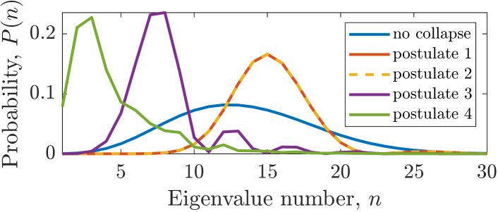
Figure 8: Comparison of probability distributions for energy eigenvalues for the different collapse postulates.

Postulate			Expected energy
No collapse			13.125 GeV
Postulate 1			14.75 GeV
Postulate 2			14.62 GeV
Postulate 3			11.46 GeV
Postulate 4			5.57 GeV

Table 1: Expectation values of energy in the five postulated situations.

Note that the expectation value of energy (Table 1) for unitary evolution of the wavefunction depends on the initial wavefunction considered and those for the four collapse postulates depend on the variance of the post-collapse wavefunction. Since we have considered the standard deviation to be 0.25 in all cases, one should pay attention to the relative magnitudes rather than the absolute magnitudes of the expectation values.

The results presented in Fig. 8 and Table 1 show that, if experiments give the expectation value of energy larger than what is predicted by standard quantum mechanics for this system, then Postulate 1 or 2 may be true, and if they give a lower value, Postulate 3 or 4 may be true.

4.2 Probability distribution of position values

We have computed the distribution of position values obtained through 10,000 time-steps. These are plotted in Fig. 9.

(a)
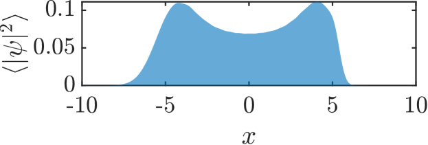
(b)
(c)
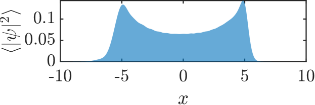
(d)
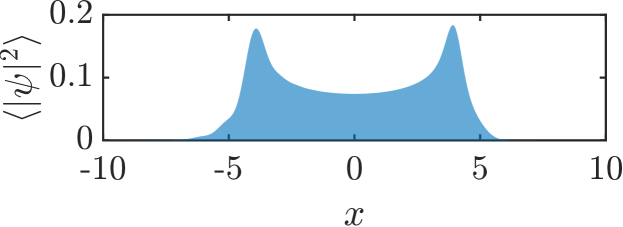
(e)

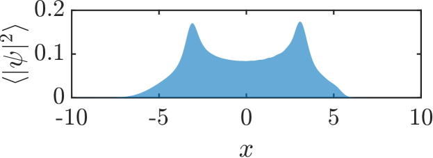
Figure 9: The averaged probability density functions of the position of the particle (a) without collapse, (b) for postulate 1, (c) for postulate 2, (d) for postulate 3, and (e) for postulate 4.

Postulate			Mean			SD
No collapse			-0.2662			3.4963
Postulate 1			4.8217			1.1296
Postulate 2			-0.2630			3.6354
Postulate 3			-0.0657			3.1330
Postulate 4			-0.0812			2.8818

Table 2: Mean and standard deviations of the time averaged PDFs for the different collapse postulates.

It is found that if Postulate 1 is true, there is only one peak in the probability distribution and in all other cases there are two peaks. For unitary evolution without collapse, the two peaks are of almost the same height while in the other cases they are of dissimilar heights. Table 2 gives the mean and standard deviation of the distributions for the five cases shown in Fig. 9.

5 The wall represented by another particle

In the previous section, we considered how a macroscopic object like a spring-supported soft wall might bring about the collapse of the wavefunction of a particle. We now ask: What happens if the wall is represented by another microscopic particle? Can such an interaction between two quantum particles lead to collapse of their wavefunctions?

We consider the soft wall to be made up of a particle of mass $m_{2}$, oscillating in its own harmonic potential with spring constant $k_{2}$ (Fig. 10). Classically, this corresponds to the situation where the soft wall is no longer massless. Each particle is in their own harmonic potential wells and there is no interaction between them except when they meet. We assume that they may meet when their wavefunctions have a significant overlap. We postulate that an interaction of this kind can also lead to the collapse of their wavefunctions, and work out the implications of such an assumption.

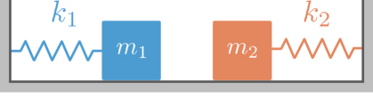
Figure 10: Classical analog of the two-particle system.

The Hamiltonian of the system is

$$\hat{H}=-\frac{\hbar^{2}}{2m_{1}}\frac{\partial^{2}}{\partial{x_{1}}^{2}}-\frac{\hbar^{2}}{2m_{2}}\frac{\partial^{2}}{\partial{x_{2}}^{2}}+\frac{k_{1}x_{1}^{2}}{2}+\frac{k_{2}x_{2}^{2}}{2}$$ (4)

where $k_{1}$ and $k_{2}$ are the spring constants of the two harmonic oscillator potentials; $m_{1}$ and $m_{2}$ are the masses of the two particles. Since there is no interaction term in this Hamiltonian, the state of the two-particle system remains separable:

$$\psi(x_{1},x_{2})=\psi_{1}(x_{1})\leavevmode\nobreak\ \psi_{2}(x_{2})$$

The evolution is governed by their single-particle Schrödinger equations

$$i\hbar\frac{\partial\psi_{1}}{\partial t}=\left[-\frac{\hbar^{2}}{2m_{1}}\frac{\partial^{2}}{\partial{x_{1}}^{2}}+\frac{k_{1}x_{1}^{2}}{2}\right]\psi_{1}$$ (5)

and

$$i\hbar\frac{\partial\psi_{2}}{\partial t}=\left[-\frac{\hbar^{2}}{2m_{2}}\frac{\partial^{2}}{\partial{x_{2}}^{2}}+\frac{k_{2}x_{2}^{2}}{2}\right]\psi_{2}$$ (6)

except at instants when the wavefunctions collapse.

For numerical simulations, the harmonic potentials are taken to be centered at $-2$ and $+2$, and the initial states of the two particles are Gaussians centred at $-5$ and $+5$ respectively with a standard deviation of 1.

5.1 No collapse

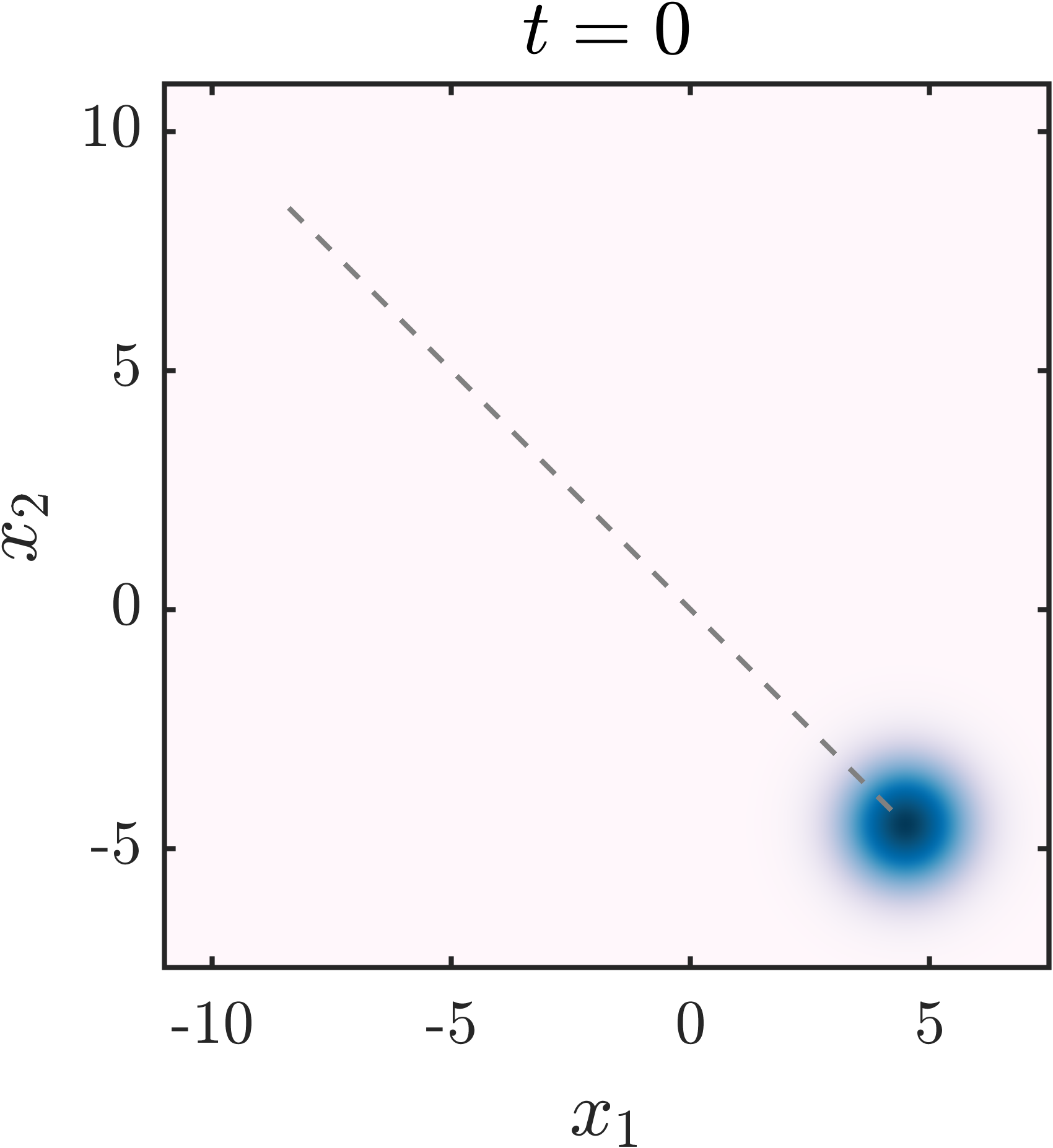
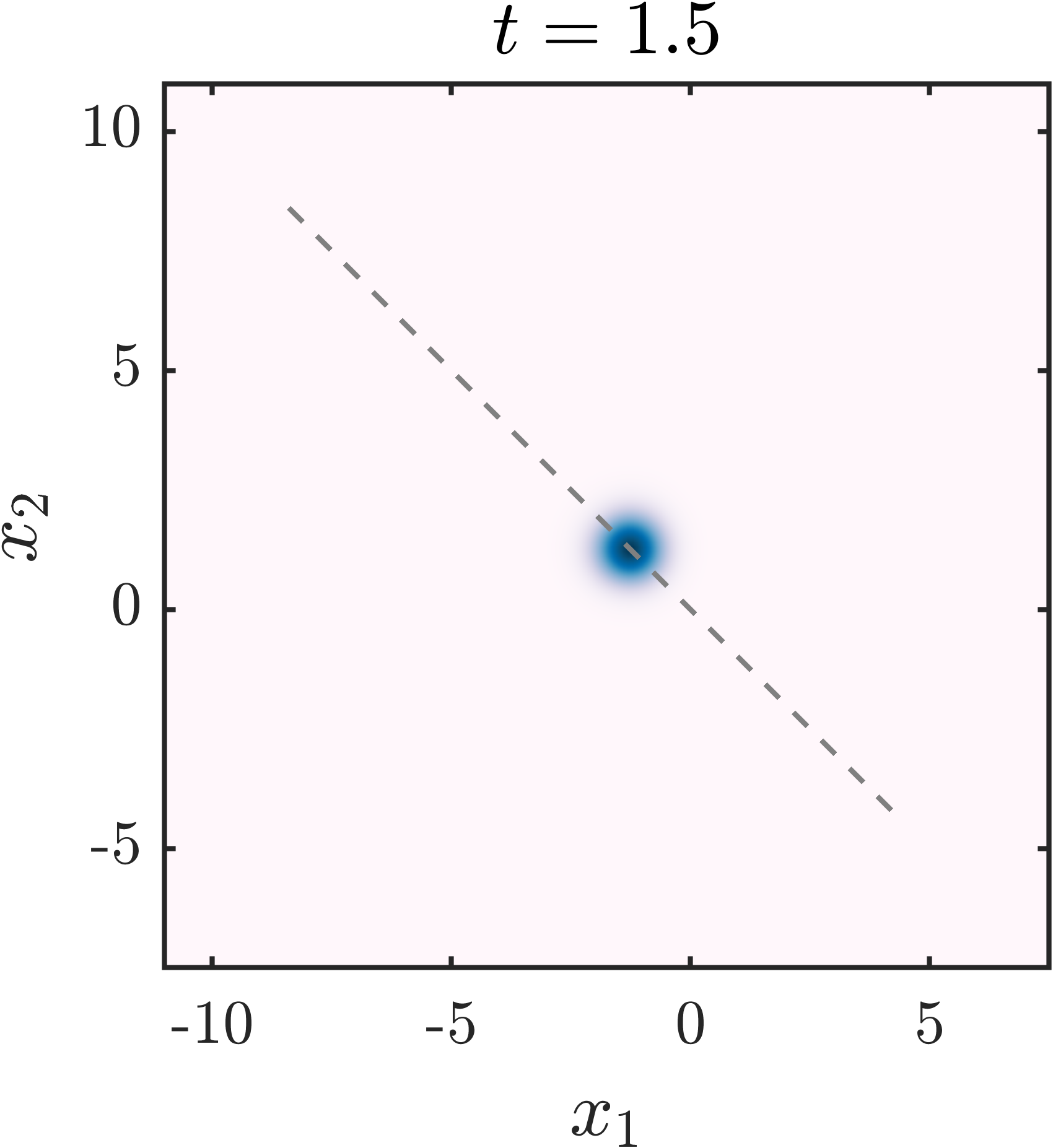
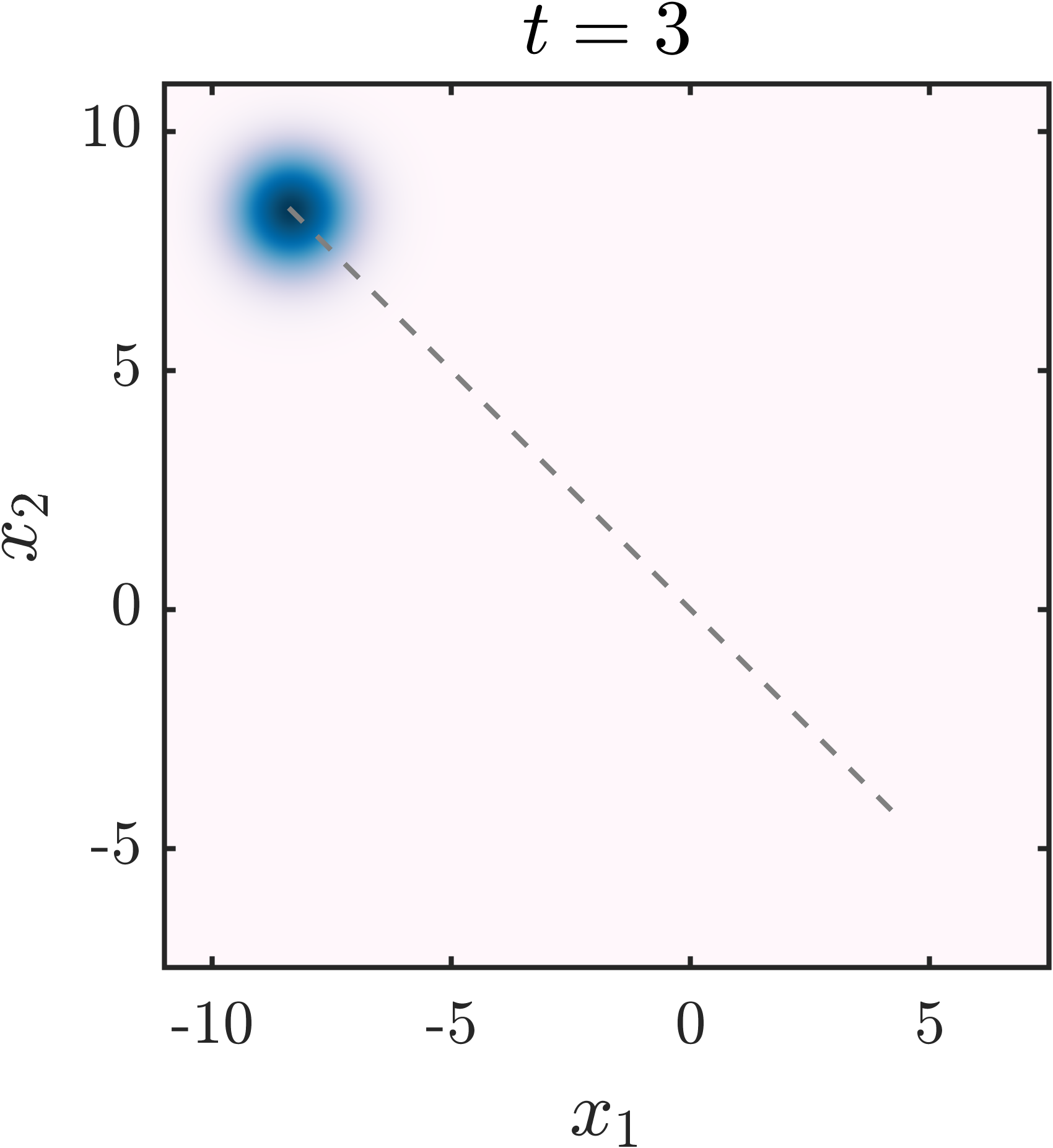
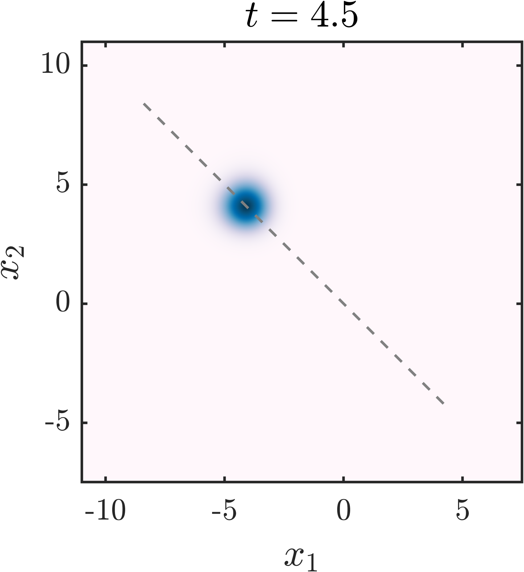
Figure 11: Evolution of the two-particle probability density $|\psi(x_{1},x_{2})|^{2}$ at four time instants for the no-collapse case. The dashed line is the locus of the expected position.

According to standard quantum mechanics, a system collapses into an eigenstate only when a measurement takes place. So, in the scenario we contemplate, the standard formulation predicts no collapse. To compare our collapse theories with the orthodox quantum mechanical prediction, we first simulate the system without wavefunction collapse. The contour plots of the probability distribution ($|\psi(x_{1},x_{2})|^{2}$) for such an evolution can be seen in Fig. 11. The distribution periodically spreads and shrinks while its mean value moves along the dashed line shown. The evolution is completely periodic for rational ${\omega_{1}}/{\omega_{2}}$ (where $\omega=\sqrt{{k}/{m}}$) and quasiperiodic otherwise.

5.2 Energy conserved collapse

A shortcoming of orthodox quantum mechanics and dynamical collapse theories like GRW and CSL is that they violate conservation of energy. Dynamical collapse theories make small but testable predictions for these violations [14] which can be used to validate and narrow down the free parameters in these models. Since no such violation has yet been reported, we invoke Occam’s razor and assume that energy is indeed conserved. We hence postulate two different collapse processes that respect the conservation of energy. The first of the two processes conserves energy of each individual particle, while the second conserves the total energy of the system through the collapse process. These processes are detailed below. The expectation value of energy is given by

$$\langle E\rangle=\langle\psi|\hat{H}|\psi\rangle=\int_{-\infty}^{\infty}\psi^{*}(x)\,\hat{H}\,\psi(x)\,\mathrm{d}x$$

For a particle described by a Gaussian wavepacket centered at $a$ with SD

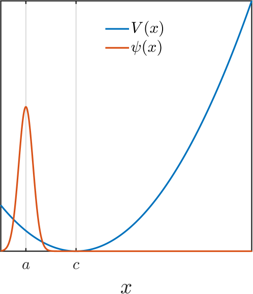
Figure 12: A Gaussian wavepacket in a translated harmonic potential. The centers of the wavepacket and the potential are $a$ and $c$ repectively.

$\sigma$

$$\psi(x)=\frac{1}{\sqrt{\sqrt{2\pi}\sigma}}\exp\left[{-\frac{(x-a)^{2}}{4\sigma^{2}}}\right]$$

in the translated harmonic potential (Fig. 12) for which the Hamiltonian is

$$\hat{H}=-\frac{\hbar^{2}}{2m}\frac{\partial^{2}}{\partial x^{2}}+\frac{1}{2}k(x-c)^{2},$$

the expectation value of energy is

$$\langle E\rangle= \int_{-\infty}^{\infty}\psi^{*}(x)\,\hat{H}\leavevmode\nobreak\ \psi(x)\,\mathrm{d}x$$

$$= \int_{-\infty}^{\infty}\frac{1}{\sigma\sqrt{2\pi}}\mathrm{e}^{-\frac{(x-a)^{2}}{4\sigma^{2}}}\leavevmode\nobreak\ \left[-\frac{\hbar^{2}}{2m}\frac{\partial^{2}}{\partial x^{2}}+\frac{1}{2}k(x-c)^{2}\right]\leavevmode\nobreak\ \mathrm{e}^{-\frac{(x-a)^{2}}{4\sigma^{2}}}\leavevmode\nobreak\ \mathrm{d}x$$

$$= \int_{-\infty}^{\infty}\frac{1}{2\sigma\sqrt{2\pi}}\mathrm{e}^{-\frac{(x-a)^{2}}{2\sigma^{2}}}\leavevmode\nobreak\ \left[-\frac{\hbar^{2}\left\{(x-a)^{2}-2\sigma^{2}\right\}}{4m\sigma^{4}}+k(x-c)^{2}\right]\leavevmode\nobreak\ \mathrm{d}x$$

which can be integrated using Gaussian integrals to give

$$\langle E\rangle=\frac{k}{2}\left\{\sigma^{2}+(a-c)^{2}+\frac{\hbar^{2}}{4mk\sigma^{2}}\right\}.$$

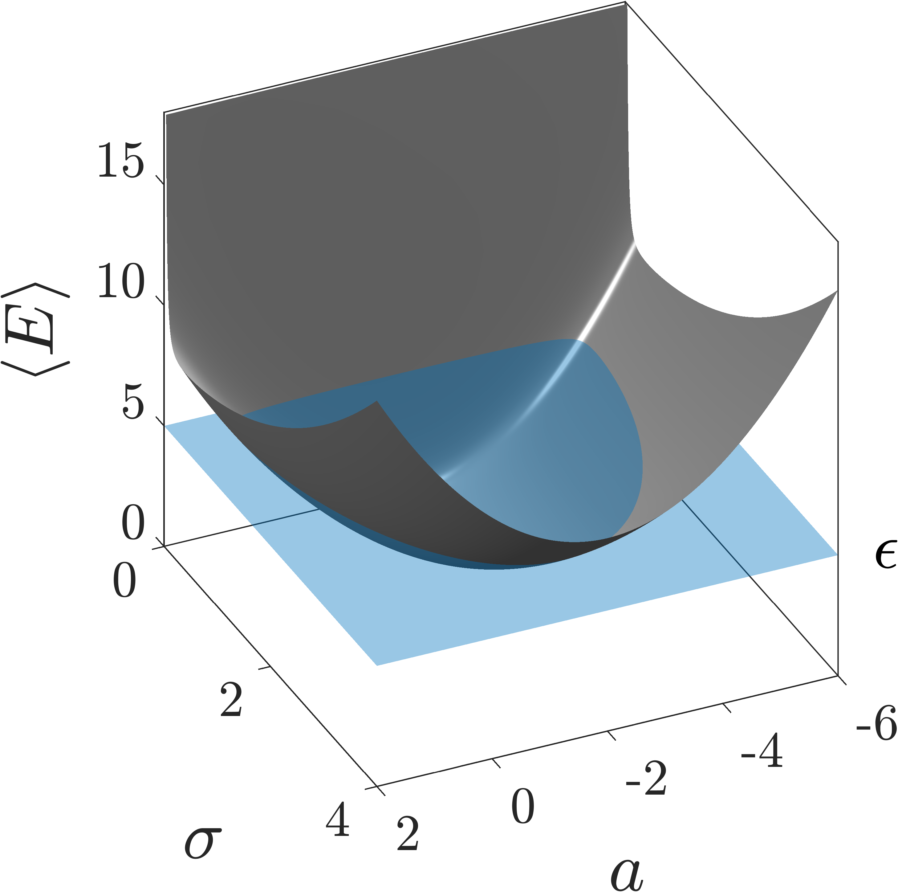
(a)

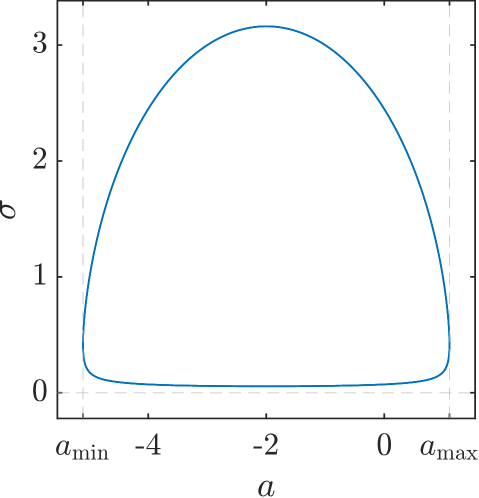
          (b)

Figure 13: Dependence of the expected energy $\langle E\rangle$ on the mean position $a$ and standard deviation $\sigma$ of the Gaussian wavepacket (gray) and surface of constant energy $\epsilon$ (blue) (a), which intersects the former surface along the curve in (b). $k=m=1$, $c=-2$.

The dependence of the expected energy on the mean $a$ and the standard deviation $\sigma$ of the Gaussian wavepacket is plotted in Fig. 13(a). If the expected energy is constrained to a certain value, say $\epsilon$, then the possible values of $a$ and $\sigma$ get constrained to the intersection between the surfaces $\langle E\rangle(a,\sigma)$ and $\langle E\rangle=\epsilon$. The resulting family of curves parametrized by $\epsilon$ contain the families of Gaussian wavepackets having equal expected energy. An energy conserved collapse model must map points from such a curve onto some other point on the same curve. The curves in question are given by

$$\sigma^{2}+(a-c)^{2}+\frac{\hbar^{2}}{4mk\sigma^{2}}-\frac{2\epsilon}{k}=0.$$ (7)

It is seen that the resulting curves (Fig. 13(b)) do not extend over the entire domain of the mean position, $a$. Coupled with the fact that Gaussian wavepackets are nonzero everywhere, this implies that an energy conserved collapse to a Gaussian wavepacket in a harmonic potential imposes a constraint on the locations where the wavefunctions can collapse, even though the probability of finding both particles at these points may be non-zero. In that sense, the energy conserved collapse postulate does not strictly follow Born’s rule.

The solution of equation (7) produces the two possible values of the variance that a Gaussian wavepacket with expected energy $\epsilon$ and centered at $a$ must have

$$\sigma^{2}=\frac{\epsilon}{k}+\frac{(a-c)^{2}\pm\sqrt{\left(\frac{2\epsilon}{k}-(a-c)^{2}\right)^{2}-\frac{\hbar^{2}}{mk}}}{2}$$ (8)

5.2.1 Individual particles conserve energy

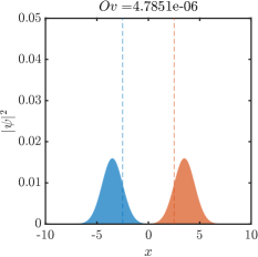
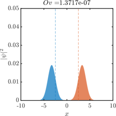
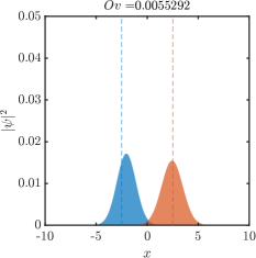
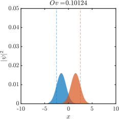
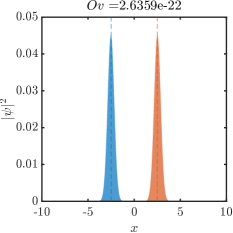
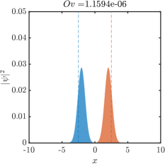
Figure 14: Time evolution of the probability distribution of the two particles at 6 time instants. The first and second particles are represented in blue and orange respectively, as are the centres of their respective harmonic potentials using dashed lines. Notice that the overlap between the distributions shown above the figures achieves a significant value in the fourth instant, triggering a collapse in the fifth instant.

The criteria we use for collapse is akin to the case of the soft impact oscillator. At a time instant $t_{i}$, the probability of collapse is the overlap between the densities of the two particles.

$$P(t_{i})=\int_{\infty}^{\infty}|\psi_{1}(x,t_{i})|^{2}\leavevmode\nobreak\ |\psi_{2}(x,t_{i})|^{2}\leavevmode\nobreak\ \text{d}x$$ (9)

For each particle to conserve energy individually, their initial expected energy has to match their expected energy after collapse. From Fig. 13(b) it is apparent that in order to conserve energy, the wavefunction cannot collapse at a position beyond the extent of the closed curve along $a$. Within this limited domain, a collapse can follow Born’s rule.

$$P(x)=\frac{{\lvert\psi(x)\rvert}^{2}}{\displaystyle\int_{a_{\text{min}}}^{a_{\text{max}}}{\lvert\psi(x^{\prime})\rvert}^{2}\leavevmode\nobreak\ \text{d}x^{\prime}}\leavevmode\nobreak\ ,\;x\in[a_{\text{min}},a_{\text{max}}]$$ (10)

The collapse process is stochastic in both position and time, governed by $P(x)$ and $P(t_{i})$. When a collapse does occur, the wavefunctions of both particles collapse simultaneously. For a particular position of collapse $a$, the energy conservation constraint allows for two different values of standard deviation $\sigma$ for the post collapse wavepacket (see Fig. 13(b)). We choose the smaller of the two to achieve maximal localization in position. Between collapses, the two particles undergo unitary evolution according to their respective Schrödinger equations. The resulting dynamics are depicted in terms of a few frames at different time instants in Fig. 14.

5.2.2 The system as a whole conserves energy

Now we consider the case where each individual particle might lose or gain energy but the expected energy of the two-particle system remains conserved through the process of collapse, i.e.,

$$\langle E\rangle_{1}+\langle E\rangle_{2}=\langle E\rangle_{\text{total}}=\text{constant.}$$

The conditions for collapse are calculated exactly as in the previous scenario. $P(t_{i})$ and $P(x)$ dictate when and where the collapse happens. In this case, however, the energy must also be redistributed between the particles.

We chose to partition the total energy between the two particles randomly. The minimum allowed energy for a particle in a harmonic oscillator potential is the ground state energy. Hence, an allowed partition must allot at least the respective ground state energy to each particle. This gives us an allowed range in energy for the partition. The partition is realized as a sample from a uniform distribution in the allowed energy range (Fig. 15).

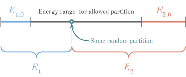
Figure 15: Schematic of the partitioning of energy between the two particles at the time of collapse. The length of the total line segment represents the total energy. The point of partition is chosen randomly on the allowed segment.

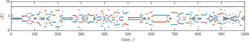
Figure 16: Expectation value of energy for the first particle (blue), second particle (orange) and the total system (black) for 1000 time steps. Energy is shuttled back and forth between the two particles, all the while conserving the total energy.

Fig. 16 shows that the expectation values of energy of the particles vary in steps whenever collapses happen, while the total energy remains conserved. This behavior may be experimentally testable.

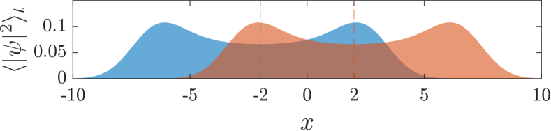
(a)

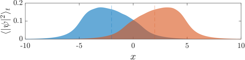
(b)

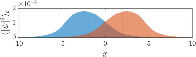
(c)

Figure 17: The time-averaged probability density functions of position of the two particles for the cases of (a) no collapse, (b) collapse with individual particles conserving energy, (c) collapse with total system conserving energy. The particles are distinguishable with the parameters : $k_{1}=k_{2}=m_{1}=m_{2}=1$. The centres of the respective potentials, $c_{1}=-2$ and $c_{2}=2$ are marked with dashed lines.

5.3 Comparison of the three cases

To quantify the differences between the three cases considered, we plot the time-averaged probability density in position for the three cases in Fig. 17. Without collapse, the average density functions have a two-humped form and are symmetric for both particles. For both the collapse postulates, the densities have single peaks and are very similar. For the case where the individual energies are conserved, the distribution functions are more skewed (i.e., the probability of finding the particles away from each other is higher) than the case where the total energy is conserved. An observed increase in the average distance between the particles can serve as a testable confirmation of the postulated collapse processes. The amount of increase can narrow down the type of interaction.

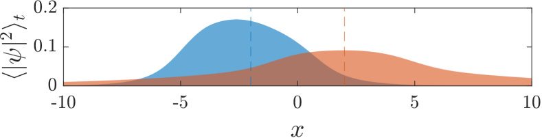
(a)

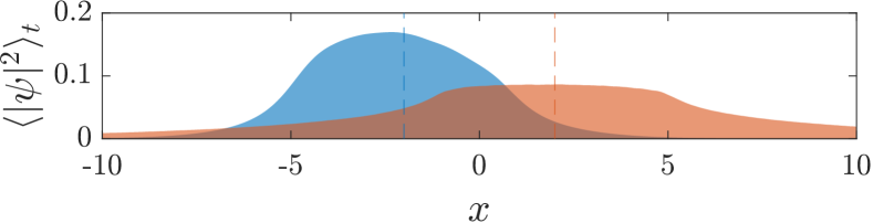
           (b)

Figure 18: The energy conserved collapse scenario when the two particles have dissimilar parameters: $k_{1}=m_{1}=1$, $k_{2}=10$ and $m_{2}=0.1$. (a) individual particles conserving energy and (b) total system conserving energy.

Fig. 18 shows the case when the $m$ and $k$ values of the two oscillators are different. In this case the qualitative behavior is similar, but the density function of the particle of lower mass has an almost flat top.

6 Conclusion

In this work we have formulated a few alternate postulates for the collapse of the wavefunction. We assume that collapse of the wavefunction of a particle does not depend on the intervention of a conscious observer. Instead, its interaction with another object, classical or quantum, may collapse its wavefunction. The probability of the occurrence of such a collapse depends on the overlap between the wavefunctions of the interacting entities.

For the situation where the particle interacts with a classical object, we have formulated four different postulates regarding the condition of collapse and the post-collapse wavefunction. For interaction among two distinguishable quantum particles, we have formulated two postulates of energy conserving wavefunction collapse.

We have proposed a model system—the quantum version of a soft-impact oscillator—and have obtained testable predictions from each postulate regarding the energy and position distribution in such a system. Our computations predict that, if an interaction with a classical object induces collapse of the wavefunction, then the probability distributions of energy and position would be different from what is predicted by standard quantum mechanics. If an interaction between two distinguishable quantum particles can induce energy-conserving collapse of their wavefunctions, then the average distance between them would tend to be larger than the distance between the centres of the two potential functions. Experimental test of the predictions would enable us to eliminate the wrong postulates.

Notice that, if any of the postulates regarding collapse of the wavefunction is supported by experiment, it will have important consequence in the foundation of quantum mechanics. It will imply that collapse of a wavefunction is a natural process that does not require conscious observation.

References

- Adler [2003] Stephen L Adler. Why decoherence has not solved the measurement problem: a response to P W Anderson. Studies in History and Philosophy of Science Part B: Studies in History and Philosophy of Modern Physics, 34(1):135–142, 2003. doi: 10.1016/S1355-2198(02)00086-2.
- Bassi and Ippoliti [2004] Angelo Bassi and Emiliano Ippoliti. Numerical analysis of a spontaneous collapse model for a two-level system. Physical Review A, 69(1):012105, 2004. doi: 10.1103/PhysRevA.69.012105.
- Bassi et al. [2013] Angelo Bassi, Kinjalk Lochan, Seema Satin, Tejinder P Singh, and Hendrik Ulbricht. Models of wave-function collapse, underlying theories, and experimental tests. Reviews of Modern Physics, 85(2):471, 2013. doi: 10.1103/RevModPhys.85.471.
- Bell [1990] John Bell. Against ‘measurement’. Physics world, 3(8):33, 1990. doi: 10.1088/2058-7058/3/8/26.
- Bell [1964] John S Bell. On the Einstein Podolsky Rosen paradox. Physics Physique Fizika, 1(3):195, 1964. doi: 10.1103/PhysicsPhysiqueFizika.1.195.
- Benatti et al. [1988] Fabio Benatti, Gian Carlo Ghirardi, Alberto Rimini, and Tullio Weber. Operations involving momentum variables in non-Hamiltonian evolution equations. Il Nuovo Cimento B (1971-1996), 101(3):333–355, 1988. doi: 10.1007/BF02828713.
- DeWitt [2015] Bryce S DeWitt. Quantum mechanics and reality. In The many worlds interpretation of quantum mechanics, pages 155–166. Princeton University Press, 2015. doi: 10.1515/9781400868056.
- Diósi [1989] Lajos Diósi. Models for universal reduction of macroscopic quantum fluctuations. Physical Review A, 40(3):1165, 1989. doi: 10.1103/PhysRevA.40.1165.
- Dolling et al. [2003] Lisa M Dolling, Arthur F Gianelli, and Glenn N Statile. The tests of time: Readings in the development of physical theory. Princeton University Press, 2003. doi: 10.2307/j.ctvcm4h07.
- Einstein et al. [1935] Albert Einstein, Boris Podolsky, and Nathan Rosen. Can quantum-mechanical description of physical reality be considered complete? Physical review, 47(10):777, 1935. doi: 10.1103/PhysRev.47.777.
- Ghirardi et al. [1986] Gian Carlo Ghirardi, Alberto Rimini, and Tullio Weber. Unified dynamics for microscopic and macroscopic systems. Physical review D, 34(2):470, 1986. doi: 10.1103/PhysRevD.34.470.
- Ghirardi et al. [1990] Gian Carlo Ghirardi, Philip Pearle, and Alberto Rimini. Markov processes in Hilbert space and continuous spontaneous localization of systems of identical particles. Physical Review A, 42(1):78, 1990. doi: 10.1103/PhysRevA.42.78.
- Ghirardi and Bassi [2020] Giancarlo Ghirardi and Angelo Bassi. Collapse Theories. In Edward N. Zalta, editor, The Stanford Encyclopedia of Philosophy. Metaphysics Research Lab, Stanford University, Summer 2020 edition, 2020.
- Goldwater et al. [2016] Daniel Goldwater, Mauro Paternostro, and PF Barker. Testing wave-function-collapse models using parametric heating of a trapped nanosphere. Physical Review A, 94(1):010104, 2016. doi: 10.1103/PhysRevA.94.010104.
- Gottwald and Melbourne [2009] Georg A Gottwald and Ian Melbourne. On the implementation of the 0–1 test for chaos. SIAM Journal on Applied Dynamical Systems, 8(1):129–145, 2009. doi: 10.1137/080718851.
- Griffiths and Schroeter [2018] David J. Griffiths and Darrell F. Schroeter. Introduction to Quantum Mechanics. Cambridge University Press, 3 edition, 2018. doi: 10.1017/9781316995433.
- Haake et al. [1992] Fritz Haake, Harald Wiedemann, and Karol Życzkowski. Lyapunov exponents from quantum dynamics. Annalen der Physik, 504(7):531–539, 1992. doi: 10.1002/andp.19925040706.
- Ing et al. [2008] James Ing, Ekaterina Pavlovskaia, Marian Wiercigroch, and Soumitro Banerjee. Experimental study of impact oscillator with one-sided elastic constraint. Philosophical Transactions of the Royal Society A: Mathematical, Physical and Engineering Sciences, 366(1866):679–705, 2008. doi: 10.1098/rsta.2007.2122.
- Joos and Zeh [1985] Eric Joos and H Dieter Zeh. The emergence of classical properties through interaction with the environment. Zeitschrift für Physik B Condensed Matter, 59(2):223–243, 1985. doi: 10.1007/BF01725541.
- Joos et al. [2013] Erich Joos, H Dieter Zeh, Claus Kiefer, Domenico JW Giulini, Joachim Kupsch, and Ion-Olimpiu Stamatescu. Decoherence and the appearance of a classical world in quantum theory. Springer Science & Business Media, 2013. doi: 10.1007/978-3-662-05328-7.
- Laha et al. [2020] Pradip Laha, S Lakshmibala, and V Balakrishnan. Bifurcations, time-series analysis of observables, and network properties in a tripartite quantum system. Physics Letters A, 384(23):126565, 2020. doi: 10.1016/j.physleta.2020.126565.
- Mendes [1991] R Vilela Mendes. Sensitive dependence and entropy for quantum systems. Journal of Physics A: Mathematical and General, 24(18):4349, 1991. doi: 10.1088/0305-4470/24/18/021.
- Milburn [1991] GJ Milburn. Intrinsic decoherence in quantum mechanics. Physical Review A, 44(9):5401, 1991. doi: 10.1103/PhysRevA.44.5401.
- Pearle [1989] Philip Pearle. Combining stochastic dynamical state-vector reduction with spontaneous localization. Physical Review A, 39(5):2277, 1989. doi: 10.1103/PhysRevA.39.2277.
- Penrose [1996] Roger Penrose. On gravity’s role in quantum state reduction. General relativity and gravitation, 28(5):581–600, 1996. doi: doi.org/10.1007/BF02105068.
- Pessoa [1997] Osvaldo Pessoa. Can the decoherence approach help to solve the measurement problem? Synthese, 113(3):323–346, 1997. URL http://www.jstor.org/stable/20117696.
- Peterka and Tondl [2004] František Peterka and Aleš Tondl. Phenomena of subharmonic motions of oscillator with soft impacts. Chaos, Solitons & Fractals, 19(5):1283–1290, 2004. doi: 10.1016/S0960-0779(03)00335-7.
- Schlosshauer [2007] Maximilian A Schlosshauer. Decoherence: and the quantum-to-classical transition. Springer Science & Business Media, 2007. doi: 10.1007/978-3-540-35775-9.