One-loop electroweak Sudakov logarithms:
a revisitation and automation

Abstract

In this work we revisit the algorithm of Denner and Pozzorini for the calculation of one-loop electroweak Sudakov logarithms and we automate it in the MadGraph5_aMC@NLO framework. We adapt the formulas for modern calculations, keeping light-quarks and photons strictly massless and dealing with infrared divergences via dimensional regularisation. We improve the approximation by taking into account additional logarithms that are angular dependent. We prove that an imaginary term has been previously omitted and we show that it cannot be in general neglected for $2\rightarrow n$ processes with $n>2$. We extend the algorithm to NLO EW corrections to squared matrix-elements that involve also QCD corrections on top of subleading LO terms. Furthermore, we discuss the usage of this algorithm for approximating physical observables and cross sections. We propose a new approach in which the QED component is consistently removed and we show how it can be superior to the commonly used approaches. The relevance of all the novelties introduced in this work is corroborated by numerical results obtained for several processes in a completely automated way. We thoroughly compare exact NLO EW corrections and their Sudakov approximations both at the amplitude level and for physical observables in high-energy hadronic collisions.

1 Introduction

After more than ten years of operation of the Large Hadron Collider (LHC), we have tremendously improved our knowledge of the fundamental interactions of elementary particles. Above all, the long-sought Higgs boson has been observed Aad:2012tfa ; Chatrchyan:2012ufa and especially its properties have been studied in detail: they have been found to be compatible with those predicted by the Standard Model (SM) Aad:2019mbh . In general, no clear and unambiguous sign of beyond-the-SM (BSM) physics has been found at colliders. In parallel, at the LHC the SM itself has been stress-tested in all its sectors: e.g., electroweak (EW) interactions, QCD dynamics and flavour physics. However, the BSM search programme at colliders is only at its initial phase. At the LHC, $20$ times more data will be collected in the next years, large part of it during the High-Luminosity (HL) runs Azzi:2019yne ; Cepeda:2019klc ; CidVidal:2018eel ; Cerri:2018ypt ; Citron:2018lsq ; Chapon:2020heu . Moreover, several options are possible for future colliders (see e.g. Ref. Gray:2021jij for a recent review), involving collisions at higher energies between a pair of protons or leptons (both electrons/positrons and muons).

The success of this ambitious research programme is interconnected with the availability of precise and reliable SM predictions. A plethora of new calculations and techniques have already appeared in the literature for improving both SM and BSM predictions. QCD radiative corrections at fixed order, going from Next-to-Leading-Order (NLO) to Next-to-NLO (NNLO) or even Next-to-NNLO ($\rm N^{3}LO$), have become available and techniques for the resummation of large logarithms appearing at fixed order have also been improved. On the other hand, an enormous effort has been done for the calculations of NLO QCD and also NLO EW corrections for processes with high-multiplicity final states. In particular, such corrections have been implemented in Monte Carlo generators and they have been even automated Kallweit:2014xda ; Frixione:2015zaa ; Chiesa:2015mya ; Biedermann:2017yoi ; Chiesa:2017gqx ; Frederix:2018nkq ; Pagani:2021iwa , at different levels in the different frameworks, using various one-loop matrix-element providers Hirschi:2011pa ; Cullen:2011ac ; Cascioli:2011va ; Actis:2012qn ; Actis:2016mpe ; Denner:2017wsf ; Buccioni:2019sur .

A particular feature of EW corrections are the so-called “Sudakov enhancements” or “Sudakov logarithms” Sudakov:1954sw , which enhance ${\cal O}(\alpha^{n})$ fixed-order corrections, the so-called ${\rm N}^{n}{\rm LO}$ EW corrections, with terms of order $\sim-\alpha^{n}\log^{k}(s/M_{W}^{2})$ with $k$ in the range $1\leq k\leq 2n$. In high-energy collisions, these logarithms involve two separate ranges of energy scales: the $W$-boson mass $M_{W}$ and the centre-of-mass energy $\sqrt{s}$. Most importantly, at variance with QCD, EW Sudakov logarithms do not cancel in IR-safe physical observables Ciafaloni:1998xg ; Ciafaloni:1999ub ; Ciafaloni:2000df ; Manohar:2014vxa , which typically are not inclusive on the additional emission of neither $W$ nor $Z$ bosons. Therefore, they induce large and negative corrections, especially in the tails of the distributions. With the future runs of the LHC, and especially with future colliders, higher energies will be probed at higher precision and therefore a reliable evaluation of such corrections and its automation in modern Monte Carlo generators is necessary.

From a theoretical point of view, a lot of work has already been done in the past for what concerns EW Sudakov logarithms from virtual corrections Beccaria:1998qe ; Ciafaloni:1998xg ; Fadin:1999bq ; Melles:2000gw ; Melles:2000ed ; Melles:2000ia ; Melles:2001mr ; Melles:2001ye ; Ciafaloni:1999ub ; Ciafaloni:2000df ; Ciafaloni:2000rp ; Ciafaloni:2000gm ; Denner:2000jv ; Melles:2001dh ; Ciafaloni:2001vt ; Ciafaloni:2001vu ; Denner:2001gw ; Denner:2003wi ; Denner:2004iz ; Denner:2006jr ; Chiu:2007yn ; Chiu:2007dg ; Chiu:2008vv ; Denner:2008yn ; Chiu:2009mg . Especially, general algorithms for the calculation at one and two-loop accuracy were derived in Refs. Denner:2000jv ; Denner:2001gw and Denner:2003wi ; Denner:2004iz ; Denner:2006jr ; Denner:2008yn , respectively. Moreover, their resummation has also been studied Kuhn:1999nn ; Fadin:1999bq ; Ciafaloni:1999ub ; Beccaria:2000jz ; Hori:2000tm ; Ciafaloni:2000df ; Denner:2000jv ; Denner:2001gw ; Melles:2001ye ; Beenakker:2001kf ; Denner:2003wi ; Pozzorini:2004rm ; Feucht:2004rp ; Jantzen:2005xi ; Jantzen:2005az ; Jantzen:2006jv ; Chiu:2007yn ; Chiu:2008vv ; Manohar:2012rs ; Bauer:2017bnh and in Refs. Chiu:2007yn ; Chiu:2008vv ; Manohar:2018kfx a general method to resum such logarithms for an arbitrary process was developed, based on the framework of soft-collinear effective theory (SCET) Bauer:2000ew ; Bauer:2000yr ; Bauer:2001ct ; Bauer:2001yt .

On the other hand, the similar case of real weak-boson emission has been addressed in Refs. Ciafaloni:2001vt ; Ciafaloni:2000rp ; Ciafaloni:2000df ; Ciafaloni:2001vu ; Ciafaloni:2001mu ; Ciafaloni:2003xf ; Ciafaloni:2005fm ; Ciafaloni:2006qu ; Ciafaloni:2008cr ; Bell:2010gi ; Ciafaloni:2010ti ; Stirling:2012ak ; Bauer:2016kkv and for specific processes on a more phenomenological level in Refs. Baur:2006sn ; Bell:2010gi ; Bern:2012vx ; Chiesa:2013yma ; Christiansen:2014kba ; Krauss:2014yaa ; Frixione:2014qaa ; Frixione:2015zaa . The resummation of double-logarithmic corrections from the real radiation has also been studied in Ref. Bauer:2016kkv and the simulation of multiple real weak boson radiation in a parton-shower approach has already been formulated and performed in Refs. Christiansen:2014kba ; Kleiss:2020rcg ; Brooks:2021kji ; Masouminia:2021kne . The SM LO collinear splitting functions Chen:2016wkt and evolution of parton fragmentation functions Bauer:2018xag are also known and phenomenological results at high energy have been studied. Finally, studies on parton-distribution-functions (PDFs) in the EW SM exist in the literature Bauer:2018arx ; Fornal:2018znf .

It is an established fact (see e.g. section 17 of Ref. Mangano:2016jyj ) that EW Sudakov logarithms from both virtual corrections and real emissions are sizeable at high energies (a few TeV’s) for several processes and, especially for the former class, resummation is necessary in order to achieve precise predictions or even just sensible results. Indeed, fixed-order corrections, precisely due to the EW Sudakov logarithms, can approach the size of $-100\%$ of the LO. In other words, in order to reach the percent accuracy, not only the exact ${\cal O}(\alpha)$ (NLO EW) corrections have to be calculated, but the Sudakov-enhanced component must be identified and resummed. Although the computation of exact NLO EW corrections is technically more involved than the case of its virtual Sudakov-logarithm subclass, only the former has been (fully) automated and implemented in Monte-Carlo’s by different collaborations Kallweit:2014xda ; Frixione:2015zaa ; Chiesa:2015mya ; Biedermann:2017yoi ; Chiesa:2017gqx ; Frederix:2018nkq ; Pagani:2021iwa . Recently, the pioneering algorithm of Denner and Pozzorini Denner:2000jv ; Denner:2001gw , which allows to calculate both single and double one-loop virtual EW Sudakov logarithms at ${\cal O}(\alpha)$, has been automated for the first time Bothmann:2020sxm in the Sherpa framework Sherpa:2019gpd . Previously, only specific (classes of) processes had been considered, as done e.g. in Ref. Chiesa:2013yma within AlpGen Mangano:2002ea .

In this work we automate the algorithm of Denner and Pozzorini Denner:2000jv ; Denner:2001gw in the MadGraph5_aMC@NLO framework Alwall:2014hca ; Frederix:2018nkq , which already allows for the fully-automated calculation of NLO QCD and EW corrections and more in general Complete-NLO predictions Frederix:2018nkq ; Pagani:2021iwa . Thus, with MadGraph5_aMC@NLO, it is now possible not only to calculate in a completely automated approach NLO EW corrections, but also their subcomponent that is typically dominant: the double and single virtual Sudakov logarithms. On the one hand, this work opens up the possibility of further building an automated framework for resumming Sudakov EW logarithms and match the result to NLO EW calculations in the MadGraph5_aMC@NLO framework. On the other hand, since virtual Sudakov logarithms are the dominant component of EW corrections and their evaluation is much faster and stable of the exact ${\cal O}(\alpha)$ result, this implementation leads also to a very good and fast approximation of NLO EW corrections at high energy.

Before implementing the algorithm of Denner and Pozzorini Denner:2000jv ; Denner:2001gw , however, we have revisited it. This work therefore does not only describe the technical steps underlying the implementation in MadGraph5_aMC@NLO, but it also provides an algorithm that is based on the one of Denner and Pozzorini and introduces relevant novelties w.r.t. it. First, we have reframed the algorithm by setting the mass of the photon and light-fermion masses exactly to zero, regularising IR divergences by mean of Dimensional Regularisation (DR), as in modern NLO EW calculations and in general Monte Carlo implementations. Second, we have identified an imaginary term that was omitted in Ref. Denner:2000jv , which however cannot be in general neglected for $2\rightarrow n$ processes with $n>2$. Third, we have modified part of the expressions in order to take into account additional angular dependences, without assuming that all the invariants are of the same size of $s$. Fourth, since (virtual) NLO EW corrections originate from both “genuine” EW corrections on top of the dominant LO contributions and QCD corrections on top of the subdominant ones, we provide additional terms for taking into account the logarithmic dependence not only of the former, as done in the original work of Denner and Pozzorini, but also of the latter. All these modifications concern the approximation of the matrix elements or, more precisely, the interference of tree-level and renormalised one-loop amplitudes leading to the ultra-violet (UV) finite virtual corrections. The fourth point mentioned before was not considered in the pioneering work of Ref. Denner:2000jv precisely because therein the focus was on the one-loop amplitudes and not their interferences with tree-level amplitudes, which is what yields the virtual contribution to NLO EW corrections. The effects of all these modifications and their validation are then showcased presenting numerical results obtained via the implementation in MadGraph5_aMC@NLO. In a fully automated way, for several different processes, we compare exact results for virtual contributions obtained via MadLoop Hirschi:2011pa , one of the modules of MadGraph5_aMC@NLO, and via the new implementation of the modified algorithm of Denner and Pozzorini for calculating one-loop virtual Sudakov logarithms.

Besides purely virtual contributions, which are unphysical and IR divergent, we also show comparisons between the Sudakov approximation and the exact NLO EW corrections for production processes in proton–proton collisions, taking into account also the necessary additional terms to achieve IR finiteness: real emission of massless particles (photons, quarks and gluons) and PDF counter-terms. We show how, for a large class of processes and IR-finite observables, at variance with the case of virtual amplitudes, the exclusion of the contribution of photons from the Denner and Pozzorini algorithm Denner:2000jv ; Denner:2001gw leads to a better approximation of NLO EW corrections. We describe in detail how the algorithm has to be altered in order to exclude the QED component (photons) and keep the purely weak one ($W$ and $Z$ bosons).

The article is organised as follows. In Sec. 2 we revisit the work of Denner and Pozzorini Denner:2000jv ; Denner:2001gw at the pure amplitude level. We set the notation, using as much as possible the same one of Ref. Denner:2000jv , and we introduce three of the main novelties mentioned before: the formulation with strictly massless light-fermions and photons, the missing imaginary term, and additional terms that better take into account angular dependences and differences among the invariants. In Sec. 3 we move to the virtual NLO EW level, considering the interference of tree-level and one-loop amplitudes. Therein, we provide the additional term for taking into account logarithms of QCD origin. In Sec. 4 we present a modification of the algorithm such that the contribution of photons and gluons is excluded. We discuss how this can be a superior approach for approximating physical (IR-safe) cross sections at NLO EW accuracy. In Sec. 5 we describe the technical steps for the implementation of the algorithm in the MadGraph5_aMC@NLO framework. We explain in detail the procedure for the generation of all the additional amplitudes that are necessary for the evaluation of the Sudakov logarithms and especially for the evaluation of the amplitudes themselves. This procedure requires new features of the code, such as the possibility to evaluate the interference between amplitudes with different external legs or numerical derivatives of the matrix elements. In Sec. 6 we provide numerical results comparing NLO EW virtual contributions obtained via MadLoop and via the new implementation of the Sudakov approximation. We show the relevance of the novelties introduced w.r.t. Ref. Denner:2000jv and at the same time we validate the new implementation. In Sec. 7 we repeat a similar comparison for physical observables from selected hadronic production processes in high-energy collisions. We discuss the numerical results and show how the exclusion of the contribution of photons leads to better approximations of the NLO EW results. Both in Sec. 6 and Sec. 7 results are obtained in a completely automated way via the new implementation in the MadGraph5_aMC@NLO framework. We give our conclusions and outlook in Sec. 8.

2 The Denner and Pozzorini algorithm revisited

We start by revisiting the pioneering work of Denner and Pozzorini Denner:2000jv ; Denner:2001gw , which provides an algorithm for calculating one-loop EW double-logarithmic (DL) and single-logarithmic (SL) corrections of the form

$$\frac{\alpha}{4\pi}\log^{2}{\frac{s}{M_{W}^{2}}}\qquad{\rm and}\qquad\frac{\alpha}{4\pi}\log{\frac{s}{M_{W}^{2}}}\,,$$ (1)

for any individual helicity configuration of a generic SM partonic processes. We introduce three novel features w.r.t. the algorithm of Ref. Denner:2000jv , which we will denoted in the following as DP algorithm:

1. In all formulas light-fermions, photons and gluons are strictly massless, as in modern higher-order calculations. In other words, IR divergences are regularised via DR, introducing a IR-regularisation scale $Q$.

2. We correct the expressions for the Subleading Soft-Collinear terms (see Secs. 2.2 and 2.4), taking into account imaginary contributions that are relevant for $2\rightarrow n$ processes with $n>2$.

3. We keep track of terms that are proportional to the (squared) logarithm of the ratio between two invariants that can be built via two different pairs of momenta among those of the external particles. Namely, using the notation that will be introduced later in this section, the terms proportional to $\log\frac{r_{kl}}{r_{k^{\prime}l^{\prime}}}$ and $\log^{2}\frac{r_{kl}}{r_{k^{\prime}l^{\prime}}}$.

In this section, we will try to use as much as possible the notation of Ref. Denner:2000jv , where the DP algorithm has been formulated. In this way the reader can easily detect the differences introduced in our work. Moreover, we will try to avoid unnecessary repetitions of the content of Ref. Denner:2000jv , but we will also define all the quantities that are entering the actual implementation in MadGraph5_aMC@NLO, which is then discussed in Sec. 5.

2.1 Range of validity and conventions

The DP algorithm strictly relies on the assumption that processes with on-shell external legs are considered and, especially, that all invariants are much larger than the gauge-boson masses. In other words, if $k$ and $l$ are two generic external particles with momenta $p_{k}$ and $p_{l}$ respectively, then

$$r_{kl}\equiv(p_{k}+p_{l})^{2}\simeq 2p_{k}p_{l}\gg M_{W}^{2}\simeq M_{H}^{2},m_{t}^{2},M_{W}^{2},M_{Z}^{2}.$$ (2)

It is interesting to notice that the condition (2) still allows for kinematic configurations with $r_{kl}\gg r_{k^{\prime}l^{\prime}}\gg M_{W}^{2}$, where the quantities $r_{kl}$ and $r_{k^{\prime}l^{\prime}}$ represent a generic pair of the many possible invariants that one can build with two external momenta. However, since the required formal accuracy consists of the DL and SL in (1), although logarithms of the form

$$\frac{\alpha}{4\pi}\log^{2}{\frac{r_{kl}}{r_{k^{\prime}l^{\prime}}}}\qquad{\rm and}\qquad\frac{\alpha}{4\pi}\log{\frac{r_{kl}}{r_{k^{\prime}l^{\prime}}}}\,,$$ (3)

are present at ${\cal O}(\alpha)$ and can be non-negligible for configurations with $r_{kl}\gg r_{k^{\prime}l^{\prime}}\gg M_{W}^{2}$, they are not taken into account. In other words, the algorithm assumes the regime (2), but large logarithms may be anyway not captured unless the condition

$$r_{kl}/r_{k^{\prime}l^{\prime}}\simeq 1$$ (4)

is satisfied for any possible pair of $r_{kl}$ and $r_{k^{\prime}l^{\prime}}$ invariants.

In fact, condition (4) is quite unrealistic for actual calculations in collider physics, since cross sections are dominated precisely by regions where one or more $r_{kl}$ invariants tend to be much smaller than $s\equiv r_{12}\gg M_{W}^{2}$. Indeed, the $r_{kl}$ invariants are related to those entering the propagators. Even if cuts are devised in order to maximise any possible value of $r_{kl}$ for a given $s$, the fulfilment of condition (4) is strictly impossible. For instance, if (2) is valid, one has that $\min(r_{kl}/s)<0.5$ for a $2\rightarrow 2$ process. This bound is even tighter and tighter for a generic $2\rightarrow n$ process with $n$ growing.

It is worth to remind the reader an important limitation of the DP algorithm. For a given process, at least one helicity configuration of the matrix element must not be mass suppressed, i.e., it must not vanish in the limit $M_{W}^{2}/s\rightarrow 0$. Indeed, such an assumption is one of the hypotheses under which the algorithm has been derived. On the other hand, most of the processes do satisfy this hypothesis, having at least one helicity configuration that is not mass suppressed. Moreover, thanks to the condition (2), helicity configurations that are not mass suppressed are by definition also dominant in the kinematic regime considered. The condition (2) also implies that processes including unstable particles and their decays cannot be treated in this approximation if physical observables are dominated by resonant configurations. Rather, the process without decays should be first considered and the decays should be then taken into account only after applying the DP algorithm.

Being aware of all the possible limitations given by the conditions (2) and (4), we describe the DP algorithm and some modifications we have introduced in order to achieve the formal leading and subleading logarithmic accuracy (LA), i.e., taking into account only enhanced DL and SL terms of the form (1), for one-loop EW virtual corrections to any SM amplitudes, in DR and therefore with possibly massless particles. The problems related to the validity of condition (4) will be also addressed, giving a pragmatic solution.

The starting point of the DP algorithm is that since all the terms considered are logarithmic, they can be expressed via the quantities

$$L(|r_{kl}|,M^{2})\equiv\frac{\alpha}{4\pi}\log^{2}{\frac{|r_{kl}|}{M^{2}}}\qquad{\rm and}\qquad l(|r_{kl}|,M^{2})\equiv\frac{\alpha}{4\pi}\log{\frac{|r_{kl}|}{M^{2}}}\,,$$ (5)

where $r_{kl}$ can be any of the invariants and $M$ any of the masses among $M_{W},M_{H},$ $m_{t}$ and $M_{Z}$, depending on the associated Feynman diagrams. Moreover, in the case of massless particles, the regularisation of the divergences will lead to logarithms of the form (5) where $M\rightarrow Q$ and $Q$ is the IR-regularisation scale. The most important point, in order to understand the novelties introduced in this section, is that the DP algorithm splits twice the logarithms of the form in (5); both splittings are connected to the modifications of the DP algorithm that we present in this work.

First, logarithms of the form in (5) are split into two classes: a symmetric and solely energy-dependent class, which is associated to the scales $M_{W}$ and $\sqrt{s}$ and parametrised by the quantities

$$L(s)\equiv L(s,M_{W}^{2})\qquad{\rm and}\qquad l(s)\equiv l(s,M_{W}^{2})\,,$$ (6)

and a remaining class of logarithms involving mass ratios and ratios of invariants. This splitting involves the imaginary component that we are going to introduce in the formulas and that is not present in Ref. Denner:2000jv . It also involves the modifications that take care of the violation of condition (4).

Second, while above the scale $M_{W}$ all one-loop EW contributions are treated in an unified approach, without separating purely QED from purely weak effects, below the $M_{W}$ scale only the QED component is present, involving logarithms between $M_{W}$ and the IR scale. In other words, for the contribution from QED loops $M_{W}$ works as a technical separator. Above $M_{W}$ we have for example (see eq. (19)) quantities parametrised via the electroweak Casimir operator $C^{{\mathrm{ew}}}$, which involves the entire $\rm SU(2)\times U(1)$ group, while below $M_{W}$ we have only quantities that involve the charges $Q_{k}$ of the external particles. The latter class of contributions is denoted by the apex “em”, standing for electromagnetic, and in Ref. Denner:2000jv it arises from the energy hierarchy $M_{H},m_{t},M_{W},M_{Z}\gg m_{f\neq t}\gg\lambda$, where $\lambda$ is the mass of the photon. In this separation the logarithms $l(M_{W}^{2},M_{Z}^{2})$, $l(m_{t}^{2},M_{W}^{2})$, and $l(M_{H}^{2},M_{W}^{2})$, similarly to the quantities $\log{(|r_{kl}|/s)}$ and $\log^{2}{(|r_{kl}|/s)}$, are neglected when they do not multiply the term $l(s)$.

In Ref. Denner:2000jv all the quantities denoted as electromagnetic (“em”) depend on $m_{f\neq t}$ and $\lambda$, which here are considered exactly equal to zero,

$$m_{f\neq t}=\lambda=0\,.$$ (7)

The consequence of (7) is that DR becomes necessary. In $D=4-2\epsilon$ dimensions, electromagnetic logarithms transform into $1/\epsilon$ poles plus finite terms and logarithms involving the IR-regularisation scale $Q$. In this context we are not interested in the structure of the IR poles, which for NLO EW corrections is discussed, e.g., in Refs. Frederix:2018nkq ; Schonherr:2017qcj ; Pagani:2021iwa ; Buccioni:2019sur ; we are interested only in the logarithmic dependence of the finite part. This can be simply derived via the substitutions

$$\log(\lambda^{2})\rightarrow\log(Q^{2})\,,\qquad\log(m^{2}_{f\neq t})\rightarrow\log(Q^{2})\,,$$ (8)

in the expressions of Ref. Denner:2000jv .

We want to comment on the dependence on $Q$, the IR-regularisation scale, which is introduced here and it is not present in the original DP algorithm. The derivation of the formulas in Ref. Denner:2000jv depends on the assumption that $\mu^{2}=s$, but therein $\mu$ is the UV-regularisation scale since all the IR divergences are regularised via $m_{f\neq t}$ and $\lambda$. However, similarly to this work, therein formulas have been derived assuming an on-shell renormalisation scheme, such as the $\alpha(M_{Z})$ or $G_{\mu}$ ones. With such a renormalisation scheme, no renormalisation-scale dependence is present for one-loop renormalised amplitudes, both if exactly calculated or using the LA. Therefore, the DP algorithm, although derived assuming a specific value for $\mu$ ($\mu^{2}=s$), returns results that do not depend on $\mu$. The substitution in (8), that we perform due to the condition (7), does not depend on the condition (2). Moreover, it affects only the regularisation of IR divergences and does not concern the UV ones. Therefore, this substitution introduces the correct dependence on $Q$ even if a common regulator for UV and IR divergences ($Q=\mu$) is used. Exceptions are discussed in Sec. 3.

Before providing the expressions necessary for automating one-loop EW Sudakov logarithms, we introduce further conventions and notations according to Ref. Denner:2000jv . Amplitudes are assumed with $n$ arbitrary external particles and all momenta $p_{k}$ incoming. Needless to say, any $2\rightarrow n-2$ amplitude can be rewritten into a $n\rightarrow 0$ amplitude via crossing symmetry. Processes are denoted as

$$\varphi_{i_{1}}(p_{1})\dots\varphi_{i_{n}}(p_{n})\rightarrow 0\,,$$ (9)

where the (anti)particles $\varphi_{i_{k}}$ are the components of the various multiplets $\varphi$ of the SM:

• $f^{\kappa}_{\sigma}$ and $\bar{f}^{\kappa}_{\sigma}$: chiral fermions and antifermions, with chiralities $\kappa={\mathrm{R}},{\mathrm{L}}$ and the isospin indices $\sigma=\pm$,

• $V_{a}=A,Z,W^{\pm}$: gauge bosons transversely (T) or longitudinally (L) polarised. Neutral gauge bosons are also denoted as $N=A,Z$,

• $\Phi_{i}$: the scalar doublet containing the Higgs particle $H$ and the neutral and charged Goldstone bosons $\chi,\phi^{\pm}$.

An important technical point of the DP algorithm is that, since the high-energy limit is assumed, the Goldstone-boson equivalence theorem can be used. In fact, with this algorithm, contributions from longitudinal gauge-bosons are always evaluated via the Goldstone-boson equivalence theorem. We will return to this point in Sec. 5.1.

Following the same notation of Ref. Denner:2000jv , the couplings of each external field $\varphi_{i_{k}}$ to the gauge bosons $V_{a}$ is denoted by ${\mathrm{i}}eI^{V_{a}}(\varphi)$, namely, ${\mathrm{i}}eI^{V_{a}}_{\varphi_{i}\varphi_{i^{\prime}}}(\varphi)$ is the coupling corresponding to the $V_{a}\bar{\varphi}_{i}\varphi_{i^{\prime}}$ vertex, with all fields that are incoming. For simplicity, in the formulas the components $\varphi_{i_{k}}$ are replaced by their indices $i_{k}$, namely, $I^{a}_{i_{k}i^{\prime}_{k}}(k)$. All the values and formulas for the quantities $I^{a}_{i_{k}i^{\prime}_{k}}(k)$, as many other terms appearing in the next sections are reported in detail in the appendices of Ref. Denner:2000jv . We do not repeat them here, but we want to warn the reader that the same exact conventions for Feynman rules have to be used in order obtain consistent results.

For any process denoted as in (9), the Born matrix element reads

$${\cal{M}}_{0}^{i_{1}\ldots i_{n}}(p_{1},\ldots,p_{n}).$$ (10)

The ${\cal O}(\alpha)$ corrections to ${\cal{M}}_{0}$ in LA, $\delta{\cal{M}}$, has the form

$$\delta{\cal{M}}^{i_{1}\ldots i_{n}}(p_{1},\ldots,p_{n})={\cal{M}}_{0}^{i^{\prime}_{1}\ldots i^{\prime}_{n}}(p_{1},\ldots,p_{n})\delta_{i^{\prime}_{1}i_{1}\ldots i^{\prime}_{n}i_{n}}.$$ (11)

Equation (11) means that the result can be written in a factorised form, but that involves Born amplitudes for different processes. The contributions to $\delta{\cal{M}}$ have different origins:

$$\delta=\delta^{{\mathrm{LSC}}}+\delta^{\SS}+\delta^{{\mathrm{C}}}+\delta^{\mathrm{PR}}.$$ (12)

The quantities $\delta^{\mathrm{LSC}}$ and $\delta^{\SS}$ are respectively the leading and subleading soft-collinear logarithms. They both emerge from the DL, which in turn originate from the eikonal approximation of one-loop diagrams where gauge bosons are exchanged between external legs and are soft-collinear. The former represents the symmetric and solely energy-dependent class of logarithms, while the latter involves mass ratios and ratios of invariants. The quantity $\delta^{\mathrm{C}}$ consists of the collinear logarithms, originating from virtual collinear gauge bosons from external lines and field renormalisation constants. The logarithms resulting from parameter renormalisation, which can be determined by the running of the couplings, correspond to the term $\delta^{\mathrm{PR}}$. In the case of longitudinally polarised bosons the equivalences

$${\cal{M}}_{0}^{\ldots W^{\pm}_{\mathrm{L}}\ldots} = {\cal{M}}_{0}^{\ldots\phi^{\pm}\ldots},$$

$${\cal{M}}_{0}^{\ldots Z_{\mathrm{L}}\ldots} = {\mathrm{i}}{\cal{M}}_{0}^{\ldots\chi\ldots},$$ (13)

are used and can be applied also for what concerns the different terms entering the definition of $\delta$.

In the following subsections we provide the formulas entering the implementation in MadGraph5_aMC@NLO, which is described in Sec. 5. We will discuss in detail only the aspects concerning the differences w.r.t. Ref. Denner:2000jv .

2.2 Logarithm splittings

As already mentioned, the DL corrections come from loop diagrams with virtual gauge bosons $V_{a}=A,Z,W^{\pm}$ connecting two external legs. In particular, they originate from regions where the gauge boson is soft and collinear to one of the external legs. Their expressions can be derived by evaluating them in the eikonal approximation.

In Ref. Denner:2000jv , DL have been in general identified as

$$L(|r_{kl}|,M^{2}) = L(s,M^{2})+2l(s,M^{2})\log{\frac{|r_{kl}|}{s}}+L(|r_{kl}|,s)$$ (14)

$$= L(s)+2l(s)\log\frac{M_{W}^{2}}{M^{2}}+2l(s)\log{\frac{|r_{kl}|}{s}}+\cdots$$

where the invariant $r_{kl}$ depends on the angle between the momenta $p_{k}$ and $p_{l}$. Equation (14) precisely represents the first of the logarithm splittings that has been mentioned before. In the first line of $\eqref{eq:angsplit}$ the quantity $L(|r_{kl}|,M^{2})$ is split into $L(s,M^{2})$, which is symmetric and energy dependent, and other two terms, of which the second can be neglected in the approximation (4). Moving to the second line, the remaining terms are further rearranged such that if $M\neq M_{W}$, the mass-ratio logarithm $\log\frac{M_{W}^{2}}{M^{2}}$ is kept only when multiplying $l(s)$. The dots at the end stand for the terms that are dropped in the splitting of the logarithms. In Ref. Denner:2000jv , the first two terms in the second line of eq. (14) are identified as the leading soft-collinear (${\mathrm{LSC}}$) contribution, which as already mentioned is angular-independent and involves only the $s/M_{W}^{2}$ ratio in the logarithms. The remaining term leads to the angular-dependent subleading soft-collinear ($\SS$) contribution.

When loop diagrams with virtual gauge bosons $V_{a}=A,Z,W^{\pm}$ connecting two external legs are evaluated in the eikonal approximation, the logarithmic dependence can be derived by the expansion of the $C_{0}$ function in the high-energy limit, namely condition (2). The expression can be found in Ref. Roth:1996pd . If the gauge boson $V$ with mass $M$ is exchanged between the external particles $\phi_{k}$ and $\phi_{l}$, the relevant quantity is, following the conventions of Ref. Roth:1996pd ,

$$C_{0}(p_{k},p_{l},M,M_{k},M_{l})\propto\frac{1}{r_{kl}}\left(\log^{2}\frac{|r_{kl}|}{M^{2}}-2i\pi\Theta(r_{kl})\log\frac{|r_{kl}|}{M^{2}}\right)\,,$$ (15)

where $\Theta$ is the Heaviside step function. It is then clear that rather than starting from $L(|r_{kl}|,M^{2})$ as in eq. (14) the correct quantity to be taken into account is

$$L(|r_{kl}|,M^{2})-2i\pi\Theta(r_{kl})l(|r_{kl}|,M^{2})\,.$$ (16)

The difference is an imaginary component that involves a term proportional to $l(s)$. For $2\rightarrow 2$ processes, this is completely irrelevant and therefore all the results presented for specific processes in Ref. Denner:2000jv are not affected by this additional term. Indeed, since $2\rightarrow 2$ tree-level amplitudes are always real (as a consequence of the optical theorem), the imaginary part of the one-loop (or Sudakov-approximated) amplitude drops out when the real part of the loop-tree interference is considered. However, this is no longer the case starting from $2\rightarrow 3$ processes, and indeed we do find that this imaginary part is not irrelevant. We therefore repeat the procedure of eq. (14) in order to identify how the impact of the term $2i\pi\Theta(r_{kl})$ translates into the DP algorithm. Moreover, we keep track of the terms that would be otherwise discarded assuming condition (4).

Starting from (16) we obtain

$$L(|r_{kl}|,M^{2})-2i\pi\Theta(r_{kl})l(|r_{kl}|,M^{2})=$$

$$=L(s,M^{2})+2l(s,M^{2})\left(\log{\frac{|r_{kl}|}{s}}-i\pi\Theta(r_{kl})\right)+L(|r_{kl}|,s)-2i\pi\Theta(r_{kl})l(|r_{kl}|,s)=$$

$$=\underbrace{L(s)+2l(s)\log\frac{M_{W}^{2}}{M^{2}}}_{\text{LSC}}+\underbrace{2l(s)\left(\log{\frac{|r_{kl}|}{s}}-i\pi\Theta(r_{kl})\right)}_{\text{SSC}}+$$ (17)

$$\qquad\underbrace{2l(M_{W}^{2},M^{2})\log{\frac{|r_{kl}|}{s}}+L(|r_{kl}|,s)-2i\pi\Theta(r_{kl})l(|r_{kl}|,s)}_{\SS^{s\rightarrow r_{kl}}}+\cdots$$

where we have dropped in the splitting of the logarithms only terms involving neither $s$ nor $r_{kl}$. In the third line of eq. (17) there are terms that are relevant for the formal expansion in LA, i.e., the correct expression to be used instead of (14). The first two terms in the sum give the ${\mathrm{LSC}}$ logarithms, while the third one contributes to the $\SS$ ones. On the contrary in the fourth line there are further terms that become relevant when $s\gg r_{kl}\gg M$, i.e., departing from condition (4). Formally, they do not enter the LA so they cannot be identified neither as LSC nor as SSC. On the other hand, since they depend on $r_{kl}$, we will take into account their contribution in the expression of the $\SS$ logarithms (Sec. 2.4). For this reason we have denoted them in eq. (17) as $\SS^{s\rightarrow r_{kl}}$.

As we will discuss in more detail in Sec. 6.2, even taking into account the $\SS^{s\rightarrow r_{kl}}$ contribution, the full control of logarithms involving the ratios of $|r_{kl}|$ invariants and $s$ cannot be achieved via the DP algorithm. We will discuss the case of a specific process for which this limitation is manifest. On the other hand, several numerical results in Sec. 6.2 and Sec. 7 clearly show how the inclusion of the $\SS^{s\rightarrow r_{kl}}$ terms substantially improves the approximation of such class of logarithms and in turn of EW virtual one-loop corrections at high energy.

2.3 LSC: Leading soft-collinear contributions

The ${\mathrm{LSC}}$ logarithms can be rearranged as a single sum over the external legs,

$$\delta^{{\mathrm{LSC}}}{\cal{M}}^{i_{1}\ldots i_{n}}=\sum_{k=1}^{n}\delta^{\mathrm{LSC}}_{i^{\prime}_{k}i_{k}}(k){\cal{M}}_{0}^{i_{1}\ldots i^{\prime}_{k}\ldots i_{n}}\,,$$ (18)

where $\delta^{\mathrm{LSC}}_{i^{\prime}_{k}i_{k}}(k)$ reads

$$\delta^{\mathrm{LSC}}_{i^{\prime}_{k}i_{k}}(k)=-\frac{1}{2}\left[C^{{\mathrm{ew}}}_{i^{\prime}_{k}i_{k}}(k)L(s)-2(I^{Z}(k))_{i^{\prime}_{k}i_{k}}^{2}\log{\frac{M_{Z}^{2}}{M_{W}^{2}}}\,l(s)+\delta_{i^{\prime}_{k}i_{k}}Q_{k}^{2}L^{\mathrm{em}}(s,Q^{2},m_{k}^{2})\right].$$ (19)

In this case, besides the term $L^{\mathrm{em}}(s,Q^{2},m_{k}^{2})$, the expression is the same as Ref. Denner:2000jv . The expressions for the electroweak Casimir operator $C^{{\mathrm{ew}}}_{i^{\prime}_{k}i_{k}}(k)$, the squared $Z$-boson coupling $(I^{Z}(k))_{i^{\prime}_{k}i_{k}}^{2}$, and the charge $Q_{k}^{2}$ for a generic particle $k$ and a specific polarisation can be found in Ref. Denner:2000jv . It is important to note that the first two quantities have indexes and can be non-diagonal. We will return to this point discussing the implementation in MadGraph5_aMC@NLO. Using DR the electromagnetic DL reads

$$L^{\mathrm{em}}(s,Q^{2},m_{k}^{2})\equiv 2l(s)\log{\left(\frac{M_{W}^{2}}{Q^{2}}\right)}+L(M_{W}^{2},Q^{2})-L^{\rm{reg}}(m_{k}^{2},Q^{2})\,,$$ (20)

with

$$L^{\rm{reg}}(m_{k}^{2},Q^{2})\equiv\begin{cases*}0&if $m_{k}^{2}=0$ \, ,\\ L(m_{k}^{2},Q^{2})&otherwise \, .\end{cases*}$$ (21)

2.4 SSC: Subleading soft-collinear contributions

Unlike the ${\mathrm{LSC}}$ terms, the $\SS$ ones remain a sum over pairs of external legs of the form

$$\delta^{\SS}{\cal{M}}^{i_{1}\ldots i_{n}}=\sum_{k=1}^{n}\sum_{l<k}\sum_{V_{a}=A,Z,W^{\pm}}\delta^{V_{a},\SS}_{i^{\prime}_{k}i_{k}i^{\prime}_{l}i_{l}}(k,l){\cal{M}}_{0}^{i_{1}\ldots i^{\prime}_{k}\ldots i^{\prime}_{l}\ldots i_{n}}\,.$$ (22)

This part is the one with the largest differences w.r.t. Ref. Denner:2000jv . The exchange of soft neutral gauge bosons contributes with

$$\delta^{A,\SS}_{i^{\prime}_{k}i_{k}i^{\prime}_{l}i_{l}}(k,l) = \left[2\left(l(s)+l(M_{W}^{2},Q^{2})\right)\left(\log{\frac{|r_{kl}|}{s}}-i\pi\Theta(r_{kl})\right)+\Delta^{s\rightarrow r_{kl}}(r_{kl},M_{W}^{2})\right]I_{i^{\prime}_{k}i_{k}}^{A}(k)I_{i^{\prime}_{l}i_{l}}^{A}(l),$$

$$\delta^{Z,\SS}_{i^{\prime}_{k}i_{k}i^{\prime}_{l}i_{l}}(k,l) = \left[2l(s)\left(\log{\frac{|r_{kl}|}{s}}-i\pi\Theta(r_{kl})\right)+\Delta^{s\rightarrow r_{kl}}(r_{kl},M_{Z}^{2})\right]I_{i^{\prime}_{k}i_{k}}^{Z}(k)I_{i^{\prime}_{l}i_{l}}^{Z}(l),$$ (23)

and charged gauge bosons yields

$$\delta^{W^{\pm},\SS}_{i^{\prime}_{k}i_{k}i^{\prime}_{l}i_{l}}(k,l)=\left[2l(s)\left(\log{\frac{|r_{kl}|}{s}}-i\pi\Theta(r_{kl})\right)+\Delta^{s\rightarrow r_{kl}}(r_{kl},M_{W}^{2})\right]I_{i^{\prime}_{k}i_{k}}^{\pm}(k)I_{i^{\prime}_{l}i_{l}}^{\mp}(l),$$ (24)

The quantity $\Delta^{s\rightarrow r_{kl}}(r_{kl},M^{2})$ is set equal to zero when the condition $\eqref{eq:rijnice}$ is assumed and the LA is applied in a strict sense, as done in Ref. Denner:2000jv . Taking instead into account the fact that $s\gg r_{kl}\gg M^{2}$, this quantity reads

$$\Delta^{s\rightarrow r_{kl}}(r_{kl},M^{2})\equiv L(|r_{kl}|,s)+2l(M_{W}^{2},M^{2})\log{\frac{|r_{kl}|}{s}}-2i\pi\Theta(r_{kl})l(|r_{kl}|,s)\,,$$ (25)

and precisely corresponds to the $\SS^{s\rightarrow r_{kl}}$ logarithms of eq. (17).

The quantities $I^{A}$, $I^{Z}$ and $I^{\pm}$ are the couplings with respectively the photon, the $Z$ boson and the $W^{\pm}$ boson, where we have omitted the indices $i^{\prime}_{j}i_{j}$. While $I^{A}$ is always diagonal in these indices, $I^{Z}$ can be non-diagonal and $I^{\pm}(k)$ is always off diagonal. The impact of the new imaginary terms proportional to $i\pi\Theta(r_{kl})$ on results obtained with the DP algorithm is directly connected to the aforementioned off-diagonal structures. Indeed the virtual contribution to NLO EW corrections involves terms of the form $2\Re({\cal{M}}_{0}\delta{\cal{M}}^{*})$, where

$$2\Re\left({\cal{M}}^{i_{1}\ldots i_{n}}_{0}(\delta{\cal{M}}^{i_{1}\ldots i_{n}})^{*}\right)\supset 2\Re\left({\cal{M}}^{i_{1}\ldots i_{n}}_{0}\left(\delta^{V_{a},\SS}_{i^{\prime}_{k}i_{k}i^{\prime}_{l}i_{l}}(k,l){\cal{M}}_{0}^{i_{1}\ldots i^{\prime}_{k}\ldots i^{\prime}_{l}\ldots i_{n}}\right)^{*}\right)\,.$$ (26)

If the $I^{V_{a}}$ entering eq. (26) via $\delta^{V_{a},\SS}$ is diagonal or both ${\cal{M}}^{i_{1}\ldots i_{n}}_{0}$ and ${\cal{M}}_{0}^{i_{1}\ldots i^{\prime}_{k}\ldots i^{\prime}_{l}\ldots i_{n}}$ are real, like in $2\rightarrow 2$ processes, the contributions of imaginary terms proportional to $i\pi\Theta(r_{kl})$ vanish, otherwise they formally contribute. It is also interesting to note that with DR and massless photons, setting $Q^{2}=s$ the entire $\delta^{A,\SS}$ contribution vanishes if we also set $\Delta^{s\rightarrow r_{kl}}(r_{kl},M_{W}^{2})=0$. This can be seen from the definition of $\delta^{A,\SS}$ in eq. (2.4). This argument will also be recalled in Sec. 3.1, where the QCD contribution to NLO EW corrections to squared matrix-element is discussed.

2.5 C: Collinear and soft single logarithms

In this section we provide the results obtained in Ref. Denner:2000jv , adapting them for the case with massless light-fermions and photons. The formula for the collinear and soft single logarithms can be written as a sum over the external particles and polarisations,

$$\delta^{{\mathrm{C}}}{\cal{M}}^{i_{1}\ldots i_{n}}=\sum_{k=1}^{n}\delta^{\mathrm{C}}_{i^{\prime}_{k}i_{k}}(k){\cal{M}}_{0}^{i_{1}\ldots i^{\prime}_{k}\ldots i_{n}}\,,$$ (27)

with $\delta^{\mathrm{C}}_{i^{\prime}_{k}i_{k}}(k)$ that depends on the external particle and polarisation $\varphi_{i_{k}}$. We provide the results in the following. The expressions for all the new terms introduced in the formulas can be found in Ref. Denner:2000jv .

Chiral fermions

Considering fermions $f^{\kappa}_{\sigma}$ with chirality $\kappa={\mathrm{R}},{\mathrm{L}}$ and isospin indices $\sigma=\pm$, the result is

$$\delta^{{\mathrm{C}}}_{f_{\sigma}f_{\sigma^{\prime}}}(f^{\kappa})=\delta_{\sigma\sigma^{\prime}}\left\{\left[\frac{3}{2}C^{{\mathrm{ew}}}_{f^{\kappa}}-\frac{1}{8s_{\mathrm{w}}^{2}}\left((1+\delta_{\kappa{\mathrm{R}}})\frac{m_{f_{\sigma}}^{2}}{M_{W}^{2}}+\delta_{\kappa{\mathrm{L}}}\frac{m_{f_{-\sigma}}^{2}}{M_{W}^{2}}\right)\right]l(s)+Q_{f_{\sigma}}^{2}l^{\mathrm{em}}(m_{f_{\sigma}}^{2})\right\},$$ (28)

where the purely electromagnetic logarithms read

$$l^{\mathrm{em}}(m_{f}^{2})\equiv\frac{1}{2}l^{\rm reg}(M_{W}^{2},m_{f}^{2})+l(M_{W}^{2},Q^{2})\,,$$ (29)

with

$$l^{\rm reg}(M_{W}^{2},m_{f}^{2})\equiv\begin{cases*}l(M_{W}^{2},Q^{2})&if $m_{f}^{2}=0$ \, ,\\ l(M_{W}^{2},m_{f}^{2})&otherwise\, .\end{cases*}$$ (30)

Transverse charged gauge bosons W

The result is

$$\delta^{\mathrm{C}}_{W^{\sigma}W^{\sigma^{\prime}}}(V_{{\mathrm{T}}})=\delta_{\sigma\sigma^{\prime}}\left[\frac{1}{2}b^{{\mathrm{ew}}}_{W}l(s)+Q_{W}^{2}l^{\mathrm{em}}(M_{W}^{2})\right]\,,$$ (31)

where $b^{{\mathrm{ew}}}_{W}$ is a coefficient of the $\beta$-function.

Transverse neutral gauge bosons A,Z

The results for symmetric and antisymmetric parts are expressed in terms of the coefficients $b^{{\mathrm{ew}}}_{NN^{\prime}}$ of the $\beta$-function. The result is

$$\delta^{\mathrm{C}}_{N^{\prime}N}(V_{{\mathrm{T}}})=\frac{1}{2}\left[E_{N^{\prime}N}b^{{\mathrm{ew}}}_{AZ}+b^{{\mathrm{ew}}}_{N^{\prime}N}\right]l(s)+\frac{1}{2}\delta_{NA}\delta_{N^{\prime}A}\delta Z^{\mathrm{em}}_{AA}.$$ (32)

where the off-diagonal $\beta$-function $b^{{\mathrm{ew}}}_{N^{\prime}N}$ coefficient is entering the expression. Since $E_{AZ}=-E_{ZA}=1$ the off-diagonal components read

$$\delta^{\mathrm{C}}_{AZ}(V_{{\mathrm{T}}})=b^{{\mathrm{ew}}}_{AZ}l(s),\qquad\delta^{\mathrm{C}}_{ZA}(V_{{\mathrm{T}}})=0.$$ (33)

The quantity $Z^{\mathrm{em}}_{AA}$ in DR reads

$$\delta Z^{\mathrm{em}}_{AA}=-\frac{4}{3}\sum_{f,i,\sigma\neq t}N_{\mathrm{C}}^{f}Q_{f_{\sigma}}^{2}l(M_{W}^{2},Q^{2})\,.$$ (34)

Longitudinally polarised gauge bosons

By means of amplitudes involving Goldstone bosons, the complete collinear corrections (27) for longitudinal gauge bosons is

$$\delta^{{\mathrm{C}}}{\cal{M}}^{\ldots W^{\pm}_{\mathrm{L}}\ldots} = \delta^{{\mathrm{C}}}_{\phi^{\pm}\phi^{\pm}}(\Phi)\,{\cal{M}}_{0}^{\ldots\phi^{\pm}\ldots}=\delta^{{\mathrm{C}}}_{\phi^{\pm}\phi^{\pm}}(\Phi)\,{\cal{M}}_{0}^{\ldots W^{\pm}_{\mathrm{L}}\ldots},$$

$$\delta^{{\mathrm{C}}}{\cal{M}}^{\ldots Z_{\mathrm{L}}\ldots} = {\mathrm{i}}\delta^{{\mathrm{C}}}_{\chi\chi}(\Phi)\,{\cal{M}}_{0}^{\ldots\chi\ldots}=\delta^{{\mathrm{C}}}_{\chi\chi}(\Phi)\,{\cal{M}}_{0}^{\ldots Z_{\mathrm{L}}\ldots}\,,$$ (35)

with

$$\delta^{\mathrm{C}}_{\phi^{\pm}\phi^{\pm}}(\Phi) = \left[2C^{{\mathrm{ew}}}_{\Phi}-\frac{N_{\mathrm{C}}^{t}}{4s_{\mathrm{w}}^{2}}\frac{m_{t}^{2}}{M_{W}^{2}}\right]l(s)+Q_{W}^{2}l^{\mathrm{em}}(M_{W}^{2}),$$

$$\delta^{\mathrm{C}}_{\chi\chi}(\Phi) = \left[2C^{{\mathrm{ew}}}_{\Phi}-\frac{N_{\mathrm{C}}^{t}}{4s_{\mathrm{w}}^{2}}\frac{m_{t}^{2}}{M_{W}^{2}}\right]l(s)\,.$$ (36)

Higgs boson

The complete correction is

$$\delta^{{\mathrm{C}}}_{HH}(\Phi)=\left[2C^{{\mathrm{ew}}}_{\Phi}-\frac{N_{\mathrm{C}}^{t}}{4s_{\mathrm{w}}^{2}}\frac{m_{t}^{2}}{M_{W}^{2}}\right]l(s)\,.$$ (37)

2.6 PR: Logarithms connected to the parameter renormalisation

The last ingredient is the logarithms related to the UV renormalisation. In Ref. Denner:2000jv they have been identified via the formula

$$\delta^{\mathrm{PR}}{\cal{M}}=\left(\frac{\delta{\cal{M}}_{0}}{\delta e}\delta e+\frac{\delta{\cal{M}}_{0}}{\delta c_{\mathrm{w}}}\delta c_{\mathrm{w}}+\frac{\delta{\cal{M}}_{0}}{\delta h_{t}}\delta h_{t}+\frac{\delta{\cal{M}}_{0}}{\delta h_{H}}\delta h_{H}^{\mathrm{eff}}\,\right)\Big{|}_{\mu^{2}=s}\,,$$ (38)

where the quantities

$$h_{t}=\frac{m_{t}}{M_{W}}\,,\qquad h_{H}=\frac{M_{H}^{2}}{M_{W}^{2}}\,,$$ (39)

are related to the top-quark Yukawa coupling and to the scalar self coupling, respectively. All the $\delta$’s are the logarithmic part of the renormalisation counter-terms of the corresponding dimensionless quantities. In the $\delta$’s, regardless of the value of $Q$ chosen for the regularising the IR divergences in the other contributions (LSC, SSC, C), the UV regularisation-scale $\mu$ must be set as $\mu^{2}=s$. Indeed, although renormalised amplitudes in an on-shell scheme do not depend on the value of the unphysical UV-regularisation scale $\mu$, the DP algorithm has been derived assuming $\mu^{2}=s$. Therefore, in order to preserve the cancellation of the $\mu$ dependence related to the UV poles, in the logarithmic part of the UV counter-terms it is necessary that $\mu^{2}=s$.

Here, we rearrange the formula in eq. (38) for practical purposes related to the implementation in MadGraph5_aMC@NLO, discussed in Sec. 5, but the results are fully equivalent with those of Ref. Denner:2000jv . In practice we rearrange it into

$$\delta^{\mathrm{PR}}{\cal{M}}=\left(\frac{\delta{\cal{M}}_{0}}{\delta\alpha}\delta\alpha+\frac{\delta{\cal{M}}_{0}}{\delta M_{W}^{2}}\delta M_{W}^{2}+\frac{\delta{\cal{M}}_{0}}{\delta M_{Z}^{2}}\delta M_{Z}^{2}+\frac{\delta{\cal{M}}_{0}}{\delta m_{t}}\delta m_{t}+\frac{\delta{\cal{M}}_{0}}{\delta n_{\rm tad}}\delta n_{\rm tad}\,\right)\Big{|}_{\mu^{2}=s}.$$ (40)

It is worth to recall that the renormalisation of masses in propagators or in couplings with mass dimension is not relevant, because those contribute only to mass-suppressed amplitudes. The parameter $n_{\rm tad}$ is a technical parameter that has the only purpose of keeping track of the appearances of the tadpole counter-term. In practice what we do is to modify Feynman rules for three-scalar and four-scalar vertices by rescaling their value by the parameter $n_{\rm tad}$, which is then set equal to one in the numerical evaluation.

We use the following formulas:

$$\frac{\delta M_{W}^{2}}{M_{W}^{2}} = -\left[b^{{\mathrm{ew}}}_{W}-4C^{{\mathrm{ew}}}_{\Phi}\right]l(\mu^{2})-\frac{N_{\mathrm{C}}^{t}}{2s_{\mathrm{w}}^{2}}\frac{m_{t}^{2}}{M_{W}^{2}}l(\mu^{2}),$$

$$\frac{\delta M_{Z}^{2}}{M_{Z}^{2}} = -\left[b^{{\mathrm{ew}}}_{ZZ}-4C^{{\mathrm{ew}}}_{\Phi}\right]l(\mu^{2})-\frac{N_{\mathrm{C}}^{t}}{2s_{\mathrm{w}}^{2}}\frac{m_{t}^{2}}{M_{W}^{2}}l(\mu^{2}),$$ (41)

and

$$\delta\alpha=\frac{2\delta Z_{e}}{4\pi} = \frac{1}{4\pi}\left(-b^{{\mathrm{ew}}}_{AA}l(\mu^{2})+2\delta Z^{{\mathrm{em}}}_{e}\right),$$ (42)

where the purely electromagnetic part reads

$$\delta Z^{{\mathrm{em}}}_{e}\equiv\begin{cases*}-\frac{1}{2}\delta Z^{\mathrm{em}}_{AA}=\frac{2}{3}\sum_{f,i,\sigma\neq t}N_{\mathrm{C}}^{f}Q_{f_{\sigma}}^{2}l(M_{W}^{2},Q^{2})&in the $\alpha(0)$ scheme\, ,\\ ~{}~{}0&in the $G_{\mu}$ or $\alpha(M_{Z})$ scheme.\end{cases*}$$ (43)

In this work, all the results are presented by adopting the $G_{\mu}$ scheme, where in the place of $\alpha$ the input parameter is $G_{\mu}$, which is related to $\alpha$ via the tree-level relation $G_{\mu}=\pi\alpha/(\sqrt{2}M_{Z}^{2}c_{\mathrm{w}}^{2}s_{\mathrm{w}}^{2})$. This translates into the substitution

$$\frac{\delta{\cal{M}}_{0}}{\delta\alpha}\delta\alpha\rightarrow\frac{\delta{\cal{M}}_{0}}{\delta G_{\mu}}\delta G_{\mu}~{}~{}{\rm with}~{}~{}\delta G_{\mu}=\frac{\delta G_{\mu}}{\delta\alpha}\delta\alpha+\frac{\delta G_{\mu}}{\delta M_{Z}^{2}}\delta M_{Z}^{2}+\frac{\delta G_{\mu}}{\delta M_{W}^{2}}\delta M_{W}^{2}\,,$$ (44)

in eq. (40).

The remaining terms are

$$\frac{\delta m_{t}}{m_{t}}=\biggl{[}\frac{1}{4s_{\mathrm{w}}^{2}}+\frac{1}{8s_{\mathrm{w}}^{2}c_{\mathrm{w}}^{2}}+\frac{3}{2c_{\mathrm{w}}^{2}}Q_{t}-\frac{3}{c_{\mathrm{w}}^{2}}Q_{t}^{2}+\frac{3}{8s_{\mathrm{w}}^{2}}\frac{m_{t}^{2}}{M_{W}^{2}}\biggr{]}l(\mu^{2})\,,$$ (45)

where on-shell renormalisation for the mass is assumed, and finally

$$\delta n_{\rm tad} = \frac{e}{2s_{\mathrm{w}}}\frac{\delta t}{M_{W}M_{H}^{2}}\,,$$ (46)

with the contribution from the tadpole renormalisation reading

$$\delta t = -T=\frac{1}{es_{\mathrm{w}}M_{W}}\biggl{[}-\frac{3}{2}M_{W}^{2}\left(\frac{M_{Z}^{2}}{c_{\mathrm{w}}^{2}}+2M_{W}^{2}\right)$$ (47)

$${}-\frac{M_{H}^{2}}{4}(2M_{W}^{2}+M_{Z}^{2}+3M_{H}^{2})+2N_{\mathrm{C}}^{t}m_{t}^{4}\biggr{]}l(\mu^{2})\,.$$

3 Sudakov logarithms and NLO EW corrections

In the previous section we have revisited the DP algorithm, which allows the calculation of electroweak DL and SL in LA for virtual scattering amplitudes. On the other hand, for collider results and in general for the calculation of physical observables, the relevant quantities are amplitudes that are either squared or interfered among them. In particular in this work our final goal is the NLO EW corrections to LO cross sections.

For any differential or inclusive cross section $\Sigma$, adopting the notation already used in Refs. Frixione:2014qaa ; Frixione:2015zaa ; Pagani:2016caq ; Frederix:2016ost ; Czakon:2017wor ; Frederix:2017wme ; Frederix:2018nkq ; Broggio:2019ewu ; Frederix:2019ubd ; Pagani:2020rsg ; Pagani:2020mov ; Pagani:2021iwa , the different contributions from the expansion in powers of $\alpha_{\scriptscriptstyle S}$ and $\alpha$ can be denoted as:

$$\Sigma_{{\rm LO}}(\alpha_{\scriptscriptstyle S},\alpha) =\Sigma_{{\rm LO}_{1}}+\cdots+\Sigma_{{\rm LO}_{k}}\,,$$ (48)

$$\Sigma_{{\rm NLO}}(\alpha_{\scriptscriptstyle S},\alpha) =\Sigma_{{\rm NLO}_{1}}+\cdots+\Sigma_{{\rm NLO}_{k+1}}\,,$$ (49)

with $k$ being process dependent and $k\geq 1$.

Each $\Sigma_{{\rm LO}_{i}}$ denotes a specific $\alpha_{\scriptscriptstyle S}^{n}\alpha^{m}$ perturbative order that can be present at LO, i.e., arising from tree-level diagrams only. On the contrary, each $\Sigma_{{\rm NLO}_{i}}$ denotes a specific NLO perturbative order to which the interferences between different classes of tree-level and one-loop diagrams can contribute. For a given process, the values of $n$ and $m$ vary for each $\Sigma_{{\rm LO}_{i}}$, but the sum $n+m$ is constant. Moreover, if $\Sigma_{{\rm LO}_{i}}\propto\alpha_{\scriptscriptstyle S}^{n}\alpha^{m}$ then $\Sigma_{{\rm LO}_{i+1}}\propto\alpha_{\scriptscriptstyle S}^{n-1}\alpha^{m+1}$, $\Sigma_{{\rm NLO}_{i}}\propto\alpha_{\scriptscriptstyle S}^{n+1}\alpha^{m}$ and $\Sigma_{{\rm NLO}_{i+1}}\propto\alpha_{\scriptscriptstyle S}^{n}\alpha^{m+1}$.

It is easy to understand that if the perturbative order of each $\Sigma_{{\rm NLO}_{i}}$ is denoted as ${\cal O}(\Sigma_{{\rm NLO}_{i}})$ then

$${\cal O}(\Sigma_{{\rm NLO}_{i}})={\cal O}(\Sigma_{{\rm LO}_{i}})\times\alpha_{\scriptscriptstyle S}={\cal O}(\Sigma_{{\rm LO}_{i-1}})\times\alpha\,.$$ (50)

Equation (50) implies something that is very well known and, e.g., has been discussed in detail in Ref. Frixione:2014qaa . If $\Sigma_{{\rm NLO}_{i}}$ involves EW corrections ($i>1$) and it is not the term with the possibly highest $\alpha$ power at NLO ($i<k+1$), then both QCD and EW loops on top of tree-level amplitudes can enter into the game. Even worse, this separation into “QCD loops” and “EW loops” is artificial and especially cannot be rigorously defined. Since one of the main features of our implementation of the DP algorithm is the possibility of comparing the DL and SL terms in LA against the exact result for NLO EW corrections, the contribution of such “QCD loops” cannot be ignored.

In LA, the contribution from one-loop corrections to the quantity $\Sigma_{{\rm NLO}_{i}}$, denoted as $\Sigma^{\rm virt}_{{\rm NLO}_{i}}$ can be written in the form

$$(\Sigma^{\rm virt}_{{\rm NLO}_{i}})\Big{|}_{\rm LA}=\Sigma_{{\rm LO}_{i-1}}\delta^{\rm EW}_{\rm LA}+\Sigma_{{\rm LO}_{i}}\delta^{\rm QCD}_{\rm LA}\,.$$ (51)

In the following section we provide the necessary ingredients for taking into account single and double-logarithmic enhanced contribution of QCD origin in the computation of $\Sigma_{{\rm NLO}_{2}}$, what is typically dubbed in the literature as “NLO EW corrections”. The case of the Complete-NLO, i.e. the complete set of $\Sigma_{{\rm NLO}_{i}}$ contributions, is left for future work. In practice, what is discussed in this work is sufficient for both the case of $\Sigma_{{\rm NLO}_{2}}$ and $\Sigma_{{\rm NLO}_{k+1}}$, since the latter never receives contributions from “QCD loops”, as can be seen from eq. (50).

The quantity $\delta^{\rm EW}_{\rm LA}$ is what is calculated via the DP algorithm revisited in Sec. 2 and summarised in eqs. (10)–(12). For the case of $\Sigma_{{\rm NLO}_{2}}$, or equivalently the case $\Sigma_{{\rm NLO}_{k+1}}$, if ${\cal{M}}_{0}$ is the amplitude that once squared leads to $\Sigma_{{\rm LO}_{1}}$, or equivalently $\Sigma_{{\rm LO}_{k}}$, then

$$\delta^{\rm EW}_{\rm LA}\equiv\frac{2\Re({\cal{M}}_{0}\delta{\cal{M}}^{*})}{|{\cal{M}}_{0}|^{2}}\,.$$ (52)

As we said, we leave the case of the Complete-NLO for future work. In that case also eq. (52) would receive modifications since a generic $\Sigma_{{\rm LO}_{i-1}}$ term with $1<i<k$ can itself arise from the interference of amplitudes factorising different powers of $\alpha_{\scriptscriptstyle S}$ and $\alpha$.

3.1 Contributions from QCD loops

If $\Sigma_{{\rm LO}_{i}}\propto\alpha_{\scriptscriptstyle S}^{n}\alpha^{m}$, since $\Sigma_{{\rm LO}_{i+1}}\propto\alpha_{\scriptscriptstyle S}^{n-1}\alpha^{m+1}$ then $\Sigma_{{\rm LO}_{i+1}}$ originates from either a squared amplitude $|{\tilde{\cal{M}}}_{0}|^{2}$ with

$${\tilde{\cal{M}}}_{0}\propto\alpha_{\scriptscriptstyle S}^{(n-1)/2}\alpha^{(m+1)/2}\,,$$ (53)

or an interference ${\tilde{\cal{M}}}_{0,1}{\tilde{\cal{M}}}_{0,2}^{*}$ of two amplitudes ${\tilde{\cal{M}}}_{0,1}$ and ${\tilde{\cal{M}}}_{0,2}$ with

$${\tilde{\cal{M}}}_{0,1} \propto \alpha_{\scriptscriptstyle S}^{(n-1+j)/2}\alpha^{(m+1-j)/2}\,,$$ (54)

$${\tilde{\cal{M}}}_{0,2} \propto \alpha_{\scriptscriptstyle S}^{(n-1-j)/2}\alpha^{(m+1+j)/2}\,.$$ (55)

with $j$ being an integer in the range $0<j\leq\min(n-1,m+1)$. Similarly to eqs. (10)–(12), where starting from the amplitude ${\cal{M}}_{0}$ the logarithmic-enhanced EW corrections are denoted as $\delta{\cal{M}}$, we can denote the logarithmic-enhanced QCD corrections to ${\tilde{\cal{M}}}_{0}$ as $\delta{\tilde{\cal{M}}}$. This implies that

$$\Sigma_{{\rm LO}_{i+1}}\propto|{\tilde{\cal{M}}}_{0}|^{2}~{}~{}{\rm or}~{}~{}\Sigma_{{\rm LO}_{i+1}}\propto 2\Re({{\tilde{\cal{M}}}_{0,1}{\tilde{\cal{M}}}_{0,2}^{*}})\,,$$ (56)

and respectively

$$\Sigma_{{\rm LO}_{i+1}}\delta^{\rm QCD}_{\rm LA}\propto 2\Re({\tilde{\cal{M}}}_{0}\delta{\tilde{\cal{M}}}^{*})~{}~{}{\rm or}~{}~{}\Sigma_{{\rm LO}_{i+1}}\delta^{\rm QCD}_{\rm LA}\propto 2\Re({\tilde{\cal{M}}}_{0,1}\delta{\tilde{\cal{M}}}_{2}^{*}+{\tilde{\cal{M}}}_{0,2}\delta{\tilde{\cal{M}}}_{1}^{*})\,.$$ (57)

In principle, following the same steps of Sec. 2, one could derive a general algorithm for obtaining $\delta{\tilde{\cal{M}}}$ starting form a generic ${\tilde{\cal{M}}}_{0}$. Indeed, besides the case of non-abelian gluon vertices, the DL and SL logarithms can be identified by looking at the purely QED part of the expressions of Sec. 2. In practice, this would lead to non-trivial terms involving colour-linked amplitudes, which are not per se problematic, but still avoidable via two simple assumptions on the value of $Q^{2}$ and $\Delta^{s\rightarrow r_{kl}}(r_{kl},M^{2})$.

As already mentioned at the end of Sec. 2.4, if one sets $Q^{2}=s$ and $\Delta^{s\rightarrow r_{kl}}(r_{kl},M^{2})=0$, as in the formal derivation of Ref. Denner:2000jv , then the SSC contribution from purely QED origin vanishes. Similarly, simplifications in the rest of the expressions of Sec. 2 happen. Setting $Q^{2}=s$ and $\Delta^{s\rightarrow r_{kl}}(r_{kl},M^{2})=0$, these simplifications are present also for the case of QCD. Especially, the SSC contribution vanishes also in the case of QCD corrections. As we will see later in Sec. 4.1, these two assumptions are innocuous for what concerns $\delta^{\rm QCD}_{\rm LA}$ in LA when physical observables are considered.

With these two assumptions, if ${\tilde{\cal{M}}}_{0}\propto\alpha_{\scriptscriptstyle S}^{n_{\alpha_{\scriptscriptstyle S}}}\alpha^{n_{\alpha}}$ we can write

$$\delta{\tilde{\cal{M}}}\equiv{\tilde{\cal{M}}}_{0}\left[\Big{(}n_{t}\,L^{t}(s)+n_{\alpha_{\scriptscriptstyle S}}\,l^{\alpha_{\scriptscriptstyle S}}(\mu_{R}^{2})-n_{g}\,l^{\alpha_{\scriptscriptstyle S}}(s)\Big{)}+\frac{\delta{\tilde{\cal{M}}}_{0}}{\delta m_{t}}(\delta m_{t})^{\rm QCD}\right]\;,$$ (58)

where $n_{t}$ and $n_{g}$ are the number of top quarks and gluons in the external legs, respectively. The quantities $L^{t}(s)$, $l^{\alpha_{\scriptscriptstyle S}}(\mu^{2})$ and $(\delta m_{t})^{\rm QCD}$ are defined as

$$L^{t}(s) \equiv \frac{C_{F}}{2}\frac{\alpha_{\scriptscriptstyle S}}{4\pi}\left(\log^{2}\frac{s}{m_{t}^{2}}+\log\frac{s}{m_{t}^{2}}\right)\,,$$ (59)

$$l^{\alpha_{\scriptscriptstyle S}}(\mu^{2}) \equiv \frac{1}{3}~{}\frac{\alpha_{\scriptscriptstyle S}}{4\pi}\log\frac{\mu^{2}}{m_{t}^{2}}\,,$$ (60)

$$(\delta m_{t})^{\rm QCD} \equiv -3C_{F}\frac{\alpha_{\scriptscriptstyle S}}{4\pi}\log\frac{s}{m_{t}^{2}}\,,$$ (61)

with $C_{F}=4/3$, and they have a very different origin, as explained in the following.

The terms proportional to $L^{t}(s)$ can be obtained by performing the substitution

$$Q^{2}_{t}\frac{\alpha}{4\pi}\rightarrow C_{F}\frac{\alpha_{\scriptscriptstyle S}}{4\pi}\,,$$ (62)

in the purely electromagnetic component of the LSC and C contributions for top quarks (eqs. (19) and (28)). The reason why the top quark is special is that we are understanding the use of the five-flavour scheme. If other fermions $f$ are treated as massive ($m_{f}\neq 0$), the corresponding logarithms with $t\rightarrow f$ should be also taken into account. This is true also for the remaining contributions discussed in this section. Conversely, for all the other massless quarks, if one sets $Q^{2}=s$ and $\Delta^{s\rightarrow r_{kl}}(r_{kl},M^{2})=0$, not only the SSC but also the LSC and C contributions to $\delta^{\rm QCD}_{\rm LA}$ vanish.

The term proportional to $l^{\alpha_{\scriptscriptstyle S}}(s)$ can be derived from the diagonal C contribution for the photon by applying the substitution (62). These logarithms are the virtual counterpart of the quasi-collinear logarithms emerging from the $g\rightarrow t\bar{t}$ splittings. The term proportional to $l^{\alpha_{\scriptscriptstyle S}}(\mu_{R}^{2})$ has instead a different origin; it is connected to the ${\rm\overline{MS}}$ renormalisation of $\alpha_{\scriptscriptstyle S}$. While the renormalisation of the EW sector can be performed without introducing a renormalisation-scale dependence, this is unavoidable in QCD. With five active flavours, the logarithmic-enhanced part of the $\alpha_{\scriptscriptstyle S}$ counter-term reads

$$\frac{\delta\alpha_{\scriptscriptstyle S}}{\alpha_{\scriptscriptstyle S}}=\frac{\alpha_{\scriptscriptstyle S}}{4\pi}\Big{[}\beta_{0}\log\frac{\mu_{R}^{2}}{Q^{2}}+\frac{2}{3}\log\frac{\mu_{R}^{2}}{m_{t}^{2}}\Big{]}\,,$$ (63)

where $\mu_{R}$ is the renormalisation scale and the quantity $\beta_{0}=11-\frac{2}{3}n_{f}$ is the leading term of the QCD $\beta$ function in the SM ($n_{f}=6$). We are assuming $Q^{2}=s$ and it is reasonable to assume also $\mu_{R}^{2}\sim s$, which let us to ignore the term proportional to $\log\frac{\mu_{R}^{2}}{Q^{2}}$ in eq. (58).

While the contribution from $\alpha_{\scriptscriptstyle S}$–renormalisation to the LA can be expressed via algebraic formulas, this is not possible in the case of $m_{t}$–renormalisation (or equivalently for any other quark that would be considered as massive), where the derivative $\delta{\tilde{\cal{M}}}_{0}/\delta m_{t}$ is entering the expression. The formula in eq. (61) has been obtained in the on-shell scheme, consistently with the EW case.

Via eqs. (58) and (57) we can finally write a compact formula for $\delta^{\rm QCD}_{\rm LA}$ entering eq. (51). If $\Sigma_{{\rm LO}_{i}}\propto\alpha_{\scriptscriptstyle S}^{n}\alpha^{m}$ and therefore $\Sigma_{{\rm LO}_{i+1}}\propto\alpha_{\scriptscriptstyle S}^{n-1}\alpha^{m+1}$, then

$$\delta^{\rm QCD}_{\rm LA}\equiv 2\left[n_{t}\,L^{t}(s)+\left(n-1\right)l^{\alpha_{\scriptscriptstyle S}}(\mu_{R}^{2})-n_{g}\,l^{\alpha_{\scriptscriptstyle S}}(s)\right]+\frac{1}{\delta\Sigma_{{\rm LO}_{i}}}\frac{\delta\Sigma_{{\rm LO}_{i}}}{\delta m_{t}}(\delta m_{t})^{\rm QCD}\,.$$ (64)

4 Sudakov logarithms and physical cross sections

What has been discussed up to this point concerns the LA of one-loop “EW corrections” (Sec. 2) and one-loop “QCD corrections” (Sec. 3.1) to amplitudes and their combination for the LA of the virtual contribution to the perturbative orders $\Sigma_{{\rm NLO}_{i}}$ with $i=2$ or $i=k+1$ (eq. (51)), in the perturbative expansion of the cross section $\Sigma$.

Both cases, amplitudes or virtual contributions, are unphysical and cannot be directly used for theoretical predictions of physical quantities. Since electromagnetic contributions are included (one-loop QED corrections), the DP algorithm leads to the LA of a quantity that is IR divergent and must be combined at least with the LA of the IR-divergent real-emission contributions. Alternatively, the DP algorithm can be slightly modified by excluding the QED contribution, which is the only one leading to unphysical quantities. While virtual QED SL and DL involve the unphysical quantity $Q$, the remaining contributions of purely weak origin involve the physical masses. Clearly, also these logarithms can be partially canceled by their real-emission counter part, the heavy-boson-radiation (HBR) of an extra $W$, $H$ or $Z$ boson, but these cancellations strongly depend on the specific set-up and the degree of inclusiveness of the observable considered, see e.g. Ref. Bell:2010gi . In other words, while photon and gluon emissions and real radiation of light quarks are unavoidable contributions for obtaining IR-finite predictions, the HBR is not necessary for the sake of IR finiteness. The contribution of HBR may be also relevant for the LA of the entire $\Sigma_{{\rm NLO}_{i}}$ prediction, but this critically depends on the process and the set-up considered.

In the literature, e.g. in the recent work of Ref. Bothmann:2020sxm or in Ref. Chiesa:2013yma , this problem has been circumvented by dropping the contributions tagged as “em” in the DP algorithm, namely those involving the ratios $M_{W}^{2}/\lambda^{2}$ or $M_{W}^{2}/m_{f}^{2}$, in the original formulation, or equivalently the ratio $M_{W}^{2}/Q^{2}$ in this work. We believe this approach is artificial and based on a wrong interpretation of the role of $M_{W}$ in the DP algorithm. While the DL and SL induced by $W$ and $Z$ boson loops (the $L(|r_{kl}|,M^{2})$ and $l(|r_{kl}|,M^{2})$ terms with $M=M_{W},M_{Z}$) are physical, in the case of QED $M_{W}$ is only a technical separator used in order to split the logarithms according to the logic discussed in Sec. 2.2. Bypassing the problem of IR finiteness by simply removing the logarithms involving $M_{W}$ and the IR scale is therefore an approach mostly driven by simplicity.

We propose a more rigorous approach for avoiding IR sensitivity in the implementation of the DP algorithm for physical cross sections. We will denote this approach as $\rm SDK_{\rm weak}$, where SDK is an abbreviation for Sudakov. The $\rm SDK_{\rm weak}$ approach is based on the idea of selecting only the DL and SL of purely weak origin, excluding the contributions of QED corrections. Actually, for a large class of processes this approach leads to predictions that are much closer to the exact NLO EW corrections than in the case of approaches based on the removal of all “em” terms, what we will denote from now on also as $\rm SDK_{0}$ approach. Indeed, in sufficiently inclusive observables, most of the logarithms of QED origin cancel against their real-emission counterparts.

The DP algorithm has been formulated in Ref. Denner:2000jv for one-loop amplitudes and generalised in Sec. 3 for their interference with tree-level amplitudes. From now on, we will also denote the latter case as simply the $\rm SDK$ approach. One should keep in mind that, at variance with the $\rm SDK_{\rm 0}$ and $\rm SDK_{\rm weak}$ approaches, the $\rm SDK$ one leads to IR-divergent quantities, which approximate correctly the virtual contribution to NLO EW cross sections, but that cannot be used for physical observables. We describe in the following how expressions of Secs. 2 and 3 should be modified in order to adapt the DP algorithm, which has been formulated so far for the $\rm SDK$ approach, to the $\rm SDK_{\rm weak}$ approach.

4.1 $\rm SDK_{\rm weak}$: Purely weak LA for cross sections

In general, when $W$ bosons are not involved in a process, virtual EW corrections can be divided into a QED and a purely weak component in a gauge-invariant way. QED corrections consist of all loops involving QED interactions between fermions and photons, excluding the vacuum-polarisation diagrams. The purely weak part consists of all the rest of contributions, including also the vacuum-polarisation diagrams and the renormalisation of the photon wave-function and of the fine-structure constant $\alpha$.

In order to isolate purely weak effect in DL and SL, we exclude all contributions induced by fermions and photons interactions in all formulas of Sec. 2, with the exception of those from parameter renormalisation (PR). Moreover, we exclude also DL and SL related to photons interacting with $W$ bosons as external legs. While the classification of the $W$-$\gamma$ interaction as either a purely weak or QED effect is ambiguous, the identification of the terms in the expressions of Sec. 2 that originate from such interaction is unambiguous.

The purely weak version of the DP algorithm, $\rm SDK_{\rm weak}$, can be obtained following these steps:

1. Calculate the $\delta^{\mathrm{PR}}$ in eq. (12) as in the standard SDK approach.

2. For each external particle $\varphi_{i_{k}}$ in (9), set

   $$Q_{k}=I^{A}(k)=0\,.$$ (65)

   This step alone has the effect of eliminating all the terms tagged as “em”, with the exception of $\delta Z^{\mathrm{em}}_{AA}$. It also eliminates all the SSC terms and C terms that lead to SL originating from photons, with the exception of those related to transverse $W$ bosons.

3. For each external particle $\varphi_{i_{k}}$ in (9), perform the replacement

   $$C^{{\mathrm{ew}}}_{i^{\prime}_{k}i_{k}}(k)\longrightarrow C^{{\mathrm{ew}}}_{i^{\prime}_{k}i_{k}}(k)-Q^{2}_{k}\,,$$ (66)

   with the value of $Q^{2}_{k}$ before enforcing eq. (65). This, in combination with eq. (65), has the effect of eliminating the DL due to photons.

4. Perform the replacement

   $$b^{{\mathrm{ew}}}_{W}\longrightarrow b^{{\mathrm{ew}}}_{W}-11/3\,.$$ (67)

   This has the effect of eliminating for the transverse $W$ bosons the C terms that lead to SL originating from photons.

5. Set

   $$\delta Z^{\mathrm{em}}_{AA}=0\,,$$ (68)

   and perform the replacement

   $$b^{{\mathrm{ew}}}_{AA}\longrightarrow b^{{\mathrm{ew}}}_{AA}+\frac{4}{3}\sum_{f,i,\sigma\neq t}N_{\mathrm{C}}^{f}Q_{f_{\sigma}}^{2}=b^{{\mathrm{ew}}}_{AA}+80/9\,.$$ (69)

   This has the effect of eliminating, for the photons, the C terms that lead to SL originating from light fermions.

6. Calculate the remaining terms in eq. (12) with the new redefinitions of steps 65–69.

We want to stress that, thank to the step 1, the redefinitions of steps 65–69 do not apply to all the PR contributions discussed in Sec. 2.6; for them any QED-like contribution is retained. We remind the reader that also in this context we assume the use of either the $\alpha(M_{Z})$ or $G_{\mu}$-scheme, which both have an IR structure that is ${\rm\overline{MS}}$-like, namely, IR poles are not present in the $\alpha$ counter-term, $\delta\alpha$. This difference of treatment for the PR terms, besides the definition of purely weak and QED introduced before, can also be understood in a different way. Logarithms from PR are related to UV renormalisation and do not involve IR sensitivity, as can be seen from all the equations in Sec. 2.6, which do not depend on the infrared regulator $Q$. Therefore, in order to achieve physical predictions and eliminate the $Q$ dependence, there is no need to exclude their components that are related to QED interactions. This is in contrast with the LSC, SSC and C contributions, where the QED contributions are $Q$-dependent (see eq. (19) and eq. (2.4) for respectively LSC and SSC contributions, and eq. (29), which defines the term $l^{\rm em}$ entering most of the C contributions) and therefore IR-sensitive. Moreover, while LSC, SSC and C contributions have real-emission counterparts that, together with PDF counter-terms, lead to IR finiteness and the (partial) cancellation of $Q$ dependence, this is not the case for PR contributions.

As already mentioned, in sufficiently inclusive observables, most of the logarithms of QED origin cancel against their real-emission counterparts. Thus, as we will show in Sec. 7, the purely weak version of the DP algorithm, the $\rm SDK_{\rm weak}$ approach, reproduces very well the logarithmic dependence of NLO EW predictions for differential distributions in several cases. For example, if we consider leptons or massive particles in the final state, it is easy to understand how the purely weak version of the DP can be superior when predictions for physical observables are considered.

If the real emission of photons is considered in the eikonal approximation and integrated up to the energy $E_{\gamma}=\sqrt{s}/2$, where $E_{\gamma}$ is the energy of the photon, large part of the QED logarithms cancel. For example, all the QED contributions from LSC and SSC terms are canceled exactly. There are two classes of collinear SL that are left uncanceled: those associated to final-state radiation and those associated to initial-state radiation.

The former class of SL can be eliminated by clustering photons with charged particles. In the case of massless charged particles, the clustering is anyway unavoidable for IR safety (e.g. the case of dressed leptons) and eliminates the $Q$ dependence. In the case of massive charged particles, namely top quarks and $W$ bosons, clustering is also very reasonable since in a realistic experimental set-up the separation of collinear real radiation from very boosted objects is not feasible and, from a theoretical point of view, it leads to larger uncertainties. The clustering eliminates the physical collinear SL of QED origin, which have the form $l(s,M)$, where $M$ is the mass of the massive charged particle. The latter class of SL (initial-state) are those related to the PDFs, which therefore in an exact NLO EW calculation are subtracted by the corresponding PDF counter-terms.

Both for the case of initial- and final-state collinear SL, a special case is given by the photon. Since the top quark and the $W$ boson are massive, the corresponding collinear SL associated to their contribution to $\delta Z^{\mathrm{em}}_{AA}$ are not canceled. Indeed, in the case of the initial state, no corresponding PDF counter-terms are present, since massive particles do not enter the PDF evolution. In the case of the final state, no $\gamma\rightarrow t\bar{t}$ or $\gamma\rightarrow W^{+}W^{-}$ radiation is generated for a final state giving the same signature.

In order to be on the same ground, we also remove from eq. (58) the term proportional to $L^{t}(s)$. Indeed this is canceled by the clustering of real emissions of gluons and top quarks into recombined top-quarks. At this point it is also easy to understand why in Sec. 3.1 we have said that setting $Q^{2}=s$ and $\Delta^{s\rightarrow r_{kl}}(r_{kl},M^{2})=0$ is innocuous for what concerns $\delta^{\rm QCD}_{\rm LA}$ in LA when physical observables are considered. If we lifted these two assumptions, we would obtain many more contributions to eq. (58), but they would be all canceled by the real-radiation counterparts, together with the PDF counter-terms. The presence of the term $n_{g}\,l^{\alpha_{\scriptscriptstyle S}}(s)$ can also be seen now as the gluon QCD-counterpart of the photonic uncanceled SL that have been mentioned in the previous paragraph: being massive, top quarks do not enter in the PDF counter-terms and no $g\rightarrow t\bar{t}$ is generated. We leave to future work the exploration of these effects from QCD corrections in numerical results for physical cross sections.

All in all, the modifications to eq. (58) that have to be implemented in the $\rm SDK_{\rm weak}$ approach in order approximate physical cross sections is simply:

• Set

  $$L^{t}(s)=0\,,$$ (70)

  in eq. (58).

Finally, we want to stress that the real emission of photons from electrically charged particles and of gluons from coloured particles cannot be neglected for IR-safe observables, but at high energy even the HBR may be considered and taken into account in inclusive calculations. In that case, the $\rm SDK_{weak}$ approach should be further modified. For instance, taking into account the $Z$ radiation, also the contribution of the $Z$ boson should be removed from the DP algorithm. We leave the exploration of this approach for future work.

5 Implementation in MadGraph5_aMC@NLO

The theoretical framework described in the previous sections has been implemented in MadGraph5_aMC@NLO Alwall:2014hca , specifically in the part of the code that is deputed to the calculation of NLO QCD and EW corrections and more in general Complete-NLO predictions Frederix:2018nkq ; Pagani:2021iwa . This allows a direct comparison of results in LA and at exact fixed-order, both at amplitude level and for physical observables.

We remind the reader that in MadGraph5_aMC@NLO the IR singularities are dealt with via the FKS method Frixione:1995ms ; Frixione:1997np , automated for the first time in MadFKS Frederix:2009yq ; Frederix:2016rdc . In MadGraph5_aMC@NLO one-loop amplitudes can be evaluated via different types of integral-reduction techniques (the OPP method Ossola:2006us or the Laurent-series expansion Mastrolia:2012bu ) and techniques for tensor-integral reduction Passarino:1978jh ; Davydychev:1991va ; Denner:2005nn , all automated within the module MadLoop Hirschi:2011pa . Moreover, the codes CutTools Ossola:2007ax , Ninja Peraro:2014cba ; Hirschi:2016mdz and Collier Denner:2016kdg are employed within MadLoop, which has been optimised by taking inspiration from OpenLoops Cascioli:2011va for the integrand evaluation.

As already possible in the code, NLO QCD and EW corrections can be invoked via the syntax [QCD] [QED], see Refs. Frederix:2018nkq ; Pagani:2021iwa for more details. However, now the code allows also for the evaluation of virtual one-loop Sudakov logarithms by adding after the command generate or add process the flag --ewsudakov. As we have said, the code works for the moment for ${\cal O}(\alpha)$ corrections to the $\Sigma_{{\rm LO}_{i}}$ contribution with $i=1$ and $i=k$, according to eqs. (48) and (49). In order to implement the DP algorithm in MadGraph5_aMC@NLO, three main technical features had to be implemented:

1. The generation of all the amplitudes that are necessary for the computation of the DL and SL.

2. The evaluation of the amplitudes, especially the interferences of amplitudes involving different external legs.

3. The evaluation of the derivatives of the amplitudes, which enter the formulas concerning the PR terms.

In the following subsections we address each of the previous points.

5.1 Generation of the amplitudes

We start discussing the case of a generic partonic process

$$\varphi_{i_{1}}(p_{1})\varphi_{i_{2}}(p_{2})\rightarrow\varphi_{i_{3}}(p_{3})\dots\varphi_{i_{n}}(p_{n})\,,$$ (71)

and at the end we return to the case of proton–proton collisions.

The formulas of Sec. 2, which are given for $n\rightarrow 0$ processes, can be easily reframed in terms of more common $2\rightarrow n-2$ amplitudes via crossing symmetry,

$${\cal{M}}_{i_{1}\ldots i_{n}}(p_{1},\ldots,p_{n}) \equiv {\cal{M}}(\varphi_{i_{1}}(p_{1})\dots\varphi_{i_{n}}(p_{n})\rightarrow 0)$$ (72)

$$= {\cal{M}}(\varphi_{i_{1}}(p_{1})\varphi_{i_{2}}(p_{2})\rightarrow\bar{\varphi}_{i_{3}}(-p_{3})\dots\bar{\varphi}_{i_{n}}(-p_{n}))\,.$$

As a first step, the algorithm checks if longitudinally polarised $Z$ or $W$ bosons are present in the external legs. In such a case all the possible amplitudes that can be obtained with one or more substitutions according to eq. (2.1) are generated. In other words, starting from ${\cal{M}}_{i_{1}\ldots\{n_{W}W^{\pm}\}\{n_{Z}Z\}\dots i_{n}}$, where $\{n_{W}W^{\pm}\}$ and $\{n_{Z}Z\}$ stand for $n_{W}$ and $n_{Z}$ appearances of $W$ and $Z$ bosons respectively, the amplitudes ${\cal{M}}_{i_{1}\ldots\{(n_{W}-1)W^{\pm}\}\phi^{\pm}\{n_{Z}Z\}\dots i_{n}}$ and ${\cal{M}}_{i_{1}\ldots\{nW^{\pm}\}\{(n_{Z}-1)Z\}\chi\dots i_{n}}$ are recursively generated via the substitutions

$$Z \longrightarrow \chi\,,$$ (73)

$$W^{\pm} \longrightarrow \phi^{\pm}\,,$$ (74)

up to the point that all $W$ and/or $Z$ bosons are transformed into Goldstone bosons. Clearly, any of the previous substitutions can lead to a process for which no tree-level Feynman diagram can contribute to the amplitude. Such a case is automatically detected by the code and the amplitude is not generated. From this point on, while the original amplitude ${\cal{M}}_{i_{1}\ldots\{n_{W}W^{\pm}\}\{n_{Z}Z\}\dots i_{n}}$ is retained and used for the computation of the LO cross section, the complete set of amplitudes

$${\cal{M}}_{i_{1}\ldots\{(n_{W}-k_{W})W^{\pm}\}\{k_{W}\phi^{\pm}\}\{(n_{Z}-k_{Z})Z\}\{k_{Z}\chi\}\dots i_{n}}\,,$$ (75)

with $0\leq k_{W}\leq n_{W}$ and $0\leq k_{Z}\leq n_{Z}$ is used for the following steps in the generation of the amplitudes.

As discussed in Sec. 2, the formulas for the different contributions leading to DL and SL involve amplitudes with external particles that are different from the original ones in ${\cal{M}}_{0}$. In particular, starting from the process in (9) it is necessary to generate the amplitudes for all the processes

$$\varphi_{i_{1}}(p_{1})\dots\varphi_{i^{\prime}_{k}}\dots\varphi_{i_{n}}(p_{n})\rightarrow 0\,,$$ (76)

with $1\leq k\leq n$ that can be obtained applying the substitution $\varphi_{i_{k}}\rightarrow\varphi_{i^{\prime}_{k}}$ of the form:

$$Z \longleftrightarrow A\,,$$ (77)

$$H \longleftrightarrow \chi\,.$$ (78)

With the symbol $\longleftrightarrow$ we understand that the substitution works in the two directions. Substitution (77) is necessary for the off-diagonal components of $C^{{\mathrm{ew}}}$ entering the LSC terms and of $b^{{\mathrm{ew}}}_{N^{\prime}N}$ entering the C terms. Substitution (78) is necessary for the off-diagonal components of $(I^{Z})^{2}$ entering the neutral SSC terms. Moreover it is necessary to generate also the amplitudes for the processes

$$\varphi_{i_{1}}(p_{1})\dots\varphi_{i^{\prime}_{k}}\dots\varphi_{i^{\prime}_{l}}\dots\varphi_{i_{n}}(p_{n})\rightarrow 0\,,$$ (79)

that can be obtained either applying two substitutions $\varphi_{i_{k}}\rightarrow\varphi_{i^{\prime}_{k}}$ and $\varphi_{i_{l}}\rightarrow\varphi_{i^{\prime}_{l}}$ of the form (78), again for the off-diagonal components of $(I^{Z})^{2}$ in the neutral SSC terms, or two different $\varphi_{i_{k}}\rightarrow\varphi_{i^{\prime}_{k}}$ and $\varphi_{i_{l}}\rightarrow\varphi_{i^{\prime}_{l}}$ substitutions that together do not violate charge conservation, each one of them of the form:

$$f_{\sigma} \longleftrightarrow f_{-\sigma}\,,$$ (80)

$$H \longleftrightarrow \phi^{\pm}\,,$$ (81)

$$\chi \longleftrightarrow \phi^{\pm}\,,$$ (82)

$$A \longleftrightarrow W^{\pm}\,,$$ (83)

$$Z \longleftrightarrow W^{\pm}\,.$$ (84)

The substitutions (80)–(84) originate from the purely non-diagonal structure of $I^{\pm}I^{\mp}$ entering the charged SSC terms. We remind the reader that both the substitutions (77)–(78) for the processes (76) and (80)–(84) for the processes (79) have to be performed starting from each one of the possible processes in (75) that can be obtained from (9) via the substitutions (73)–(74).

For hadronic calculations (protons in the initial state, jets, etc.) different partonic subprocesses can contribute at the Born level. Therefore, the procedure described so far has to be separately repeated for each of them.

5.2 Evaluation of the amplitudes

The evaluation of the amplitudes follows the standard procedure of the MadGraph5_aMC@NLO framework, which relies on the helicity routines supplied by Aloha deAquino:2011ub . Here, the additional complication consists in the evaluation of interferences of amplitudes that can have different particles in the respective initial and/or final state, as shown in eq. (26). As discussed in the previous section, there can be one or even two different external particles between the two interfering amplitudes. Consequently, without altering the external momenta, external particles cannot be in general on-shell in both amplitudes. In order to preserve the on-shell conditions of external legs, external momenta have to be modified for one of the two amplitudes that are interfered. We follow this approach, modifying the external momenta of the amplitude with different external states w.r.t. the Born one.

From a technical point of view, this approach is very similar to the momentum-reshuffling techniques discussed in Ref. Frixione:2019fxg , in the context of the so-called “Simplified Treatment of Resonances” (STR) that are needed to perform, e.g., computations in supersymmetric theories. In both cases, on-shell conditions are enforced by modifying part of the external momenta and the remaining ones (possibly a subset) are reshuffled in order to preserve momentum conservation. On the other hand, in this context, not only this procedure has to be applied at the amplitude level and not at the squared-amplitude level, but it is also intrinsically more articulated. While in the case of Ref. Frixione:2019fxg only one on-shell condition is enforced and involves the invariant mass of two final-state particles, in the present case one or more on-shell conditions have to be enforced and involve the kinematic mass, $\sqrt{p_{0}^{2}-|\vec{p}|^{2}}$, of one or two individual external momenta, from the initial and/or final state. Our implementation is based on the one described in detail in Sec. 5.2 of Ref. Frixione:2019fxg , on which we base the following discussion. We use the same notation for describing the technical details.

The case of only one on-shell condition for a particle in the final state can be directly derived from Sec. 5.2 of Ref. Frixione:2019fxg . Using the same notation, it can be summarised as: given a set of momenta $k_{i}$, generate a new set $\bar{k}_{i}$ where a given (final-state) particle, denoted as $\beta$, changes its mass from $m$ to $m_{\beta}=M$. The two particles labeled as $\delta$ and $\gamma$ in Ref. Frixione:2019fxg are irrelevant for our case. Among the infinite number of solutions, two options, dubbed as A and B in Ref. Frixione:2019fxg , have been considered. In the former the energy-momentum conservation is imposed by modifying all the other final-state particle momenta, while in the latter, which is the default option in the code, by changing the momenta of the initial-state particles. The case of two on-shell conditions for particles in the final state can be achieved by applying the procedure iteratively.

The case of $\beta$ being a particle in the initial state was not relevant for Ref. Frixione:2019fxg and we will briefly present it here. In this case, we have chosen to change the momentum of only the other initial-state particle, leaving the final-state ones untouched ($\bar{k}_{i}=k_{i}$ for $i\geq 3$). This implies that the centre-of-mass energy $s$ is conserved and therefore the procedure is very simple. We start with the original initial-state momenta $k_{i}$, with $i=1,2$, where the one with $i=\beta$ is going to have a new mass. Since $s$ must be conserved and we want the new momenta $\bar{k}_{i}$ collinear to the beam pipe, in the partonic centre-of-mass frame one has to simply derive the new quantity $|\bar{k}_{\beta,z}|=|\bar{k}_{3-\beta,z}|$ enforcing momentum conservation and on-shell conditions.

We conclude by commenting on the fact that, when masses are modified for both an initial-state and a final-state particle, the procedure can again be performed iteratively. However, when the default option B is used for the final-state case, since it assumes massless initial-state momenta, the case of a new mass in the final state should be considered first, and only afterwards one should consider the initial-state one.

Before moving to the next section we want to clarify that all this procedure would be unnecessary if an analytical calculation were performed and all the mass-suppressed term were discarded. This is on the other hand not possible in an automated approach. The procedure outlined here leads to a correct evaluation of all the terms that are not mass suppressed. Indeed, all the modifications of the momenta and subsequent reshuffling operations involve only scales connected to the mass of the SM particles. The differences in the kinematics before and after the procedure outlined in this section are mass suppressed themselves, leading to smaller and smaller effects when the energy inrceases. Ambiguities related to the choice of a specific reshuffling technique and to the order in which the reshuffling is performed are also mass suppressed.

5.3 Derivative of the amplitudes

As can be seen in eqs. (40) and (58), in order to compute the logarithmic contributions induced by the parameter renormalisation, the derivatives of the amplitudes w.r.t. part of the input parameters have to be calculated. Although one may in principle use dedicated Feynman rules, such as those used for generating UV counter-terms in an NLO computation, we have opted to calculate the derivatives via numerical methods. In other words, for each phase-space point, we evaluate the quantity

$$\left.\frac{\delta{\mathcal{M}}}{\delta x}\right|_{x=\bar{x}}\equiv\frac{({\mathcal{M}}|_{x=\bar{x}(1+\delta_{\bar{x}})}-{\mathcal{M}}|_{x=\bar{x}(1-\delta_{\bar{x}})})}{2\delta_{\bar{x}}}\,,$$ (85)

where $x$ is any of the variables for which the derivative has to be performed ($M_{W},M_{Z}$, etc.), $\bar{x}$ is its numerical value when the amplitudes are evaluated and $\delta_{\bar{x}}$ is a small value, which has been set to $\delta_{\bar{x}}=10^{-5}$ for the results presented in this work. The same procedure is done for $\tilde{\cal{M}}$ in eq. (58).

We have checked that this procedure has a mild impact on the speed of the code and the choice $\delta_{\bar{x}}=10^{-5}$ is excellent in terms of both stability and precision. The use of the numerical derivatives allows also to easily adapt the calculation of PR terms for possible BSM scenarios, where additional particles and couplings would be present. Moreover, at variance with what has been done in the recent automation Bothmann:2020sxm in the Sherpa framework, the SL from PR terms are calculated exactly at ${\cal O}(\alpha)$ as all the other type of DL and SL logarithms, without including spurious terms from higher orders in the $\alpha$ expansion. This fact is crucial for the systematic comparisons we are going to carry out in Secs. 6 and 7 between NLO EW exact results and their Sudakov approximations.

6 Numerical Results: matrix-element level

In this section we present numerical results obtained via the revisitation and implementation of the DP algorithm in MadGraph5_aMC@NLO, which has been described in the previous sections. We focus here on the Sudakov approximation of one-loop amplitudes and in particular on their interferences with the corresponding tree-level ones; results for cross sections of processes that are relevant at colliders are discussed in Sec. 7. We compare exact results for the finite part of the virtual contribution to the NLO EW corrections with their Sudakov approximation, what is denoted as the “SDK approach” following the notation introduced in Sec. 4. After having specified the input parameters in Sec. 6.1, we start in Sec. 6.2 by discussing the effect of the ${\SS^{s\rightarrow r_{kl}}}$ terms in eq. (17), which are relevant when the condition (4) is not satisfied. Next, in Sec. 6.3 we show the numerical relevance of the terms proportional to $2i\pi\Theta(r_{kl})$, discussed in Sec. 2.2. Then, in Sec. 6.4 we show the relevance of the QCD corrections to the subleading LO (see Sec. 3.1) in order to compare NLO EW corrections with their Sudakov approximation.

Throughout this section, we will consider only the finite part of the virtual contribution to the NLO EW corrections. It is worth recalling that, in general, the virtual contribution is IR divergent and non-physical by itself. Since we regularise IR divergences in DR, the finite part depends on the IR-regularisation scale $Q$, which we set here always as $Q^{2}=s$.

6.1 Input parameters

The results presented in this section are obtained using the following input parameters:

$$m_{Z} =91.188~{}\textrm{GeV}\,, \quad m_{W} =80.385~{}\textrm{GeV}\,, \quad m_{H} =125~{}\textrm{GeV}\,,$$

$$m_{\textrm{t}} =173.3~{}\textrm{GeV}\,, \quad G_{\mu} =1.16639\cdot 10^{-5}~{}\,\textrm{GeV}^{-2}\,, \quad\alpha_{\scriptscriptstyle S}(M_{Z}) =0.119\,.$$ (86)

All the other SM particles are treated as massless and all the decay widths are set equal to zero. Consistently with the input parameters, EW interactions are renormalised in the $G_{\mu}$-scheme and masses and wave-functions in the on-shell scheme. QCD interactions are renormalised in the ${\rm\overline{MS}}$-scheme, with the renormalisation-group running at two loops and the renormalisation scale $\mu_{R}$ set to $\mu_{R}^{2}=s$.

6.2 Impact of ${\SS^{s\rightarrow r_{kl}}}$ terms

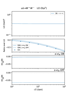
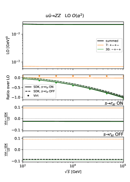
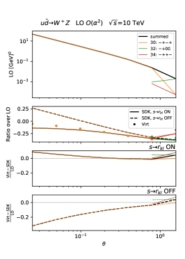
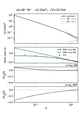
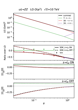
Figure 1: Comparison between exact results (dots) for ${\cal O}(\alpha)$ NLO EW virtual corrections and their LA (lines) in the case of squared matrix elements of representative $2\rightarrow 2$ processes. Solid lines include the ${\SS^{s\rightarrow r_{kl}}}$ contributions, while dashed lines do not. Upper plots show a scan in energy for a fixed $t/s$ value, while lower plots a scan in the angle $\theta$ between the momenta of the first and third particle. More details are given in the text.

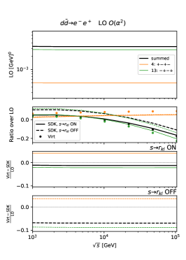
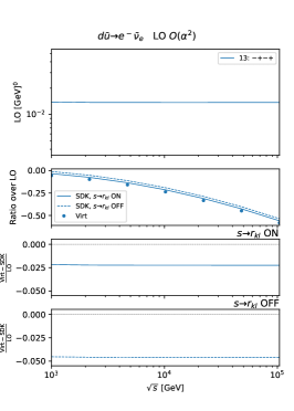
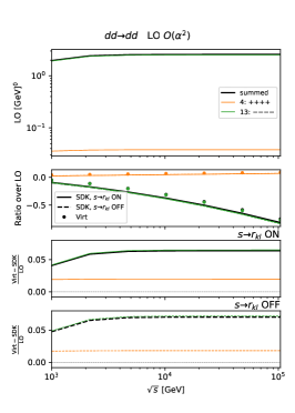
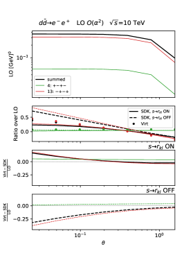
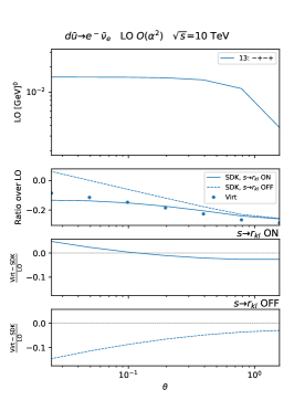
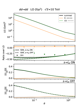
Figure 2: Same as Fig. 2, but for a different set of processes.

In this section we show numerical results for $2\rightarrow 2$ partonic processes both varying the value of $s$ and the angle $\theta$ between the first and third particle, which in turn parametrises the value of $t$. We select representative processes for which the relevant plots are displayed in Figs. 1 and 2. In both figures, the plots of each column refer to the same partonic process and the upper plots show the dependence of several quantities on the center-of-mass energy $\sqrt{s}$, while the lower plots show their $\theta$ dependence. In the following, we describe the layout of the plots and how they should be interpreted.

In the first panel we show the value of the LO squared matrix-element, separately for each leading-helicity configuration and possibly their sum if there is more than one. In order to improve the readability of the legends in the plots, therein we display not only the helicity of any external particle, but also a conventional number associated to the ordering of the helicity configurations within MadGraph5_aMC@NLO. Conventionally, leading-helicity configurations have been identified as those with a value, for their squared amplitudes, that is at least $10^{-3}$ times the one of the dominant helicity configuration. The main purpose of this conventional choice is to probe and select via a numerical method all the helicity configurations that are not mass suppressed. In the first inset we show the ratio between the ${\cal O}(\alpha)$ virtual corrections and the LO in different approximations. We display as separate dots the exact results obtained via MadLoop (Virt) for selected values of $s$, while as lines the LA approximation of Sudakov logarithms that are obtained via the new implementation of the modified DP algorithm described in this work. Dashed lines refer to the pure LA (${\SS^{s\rightarrow r_{kl}}}$ terms not included), denoted in the plots as “${\rm SDK},s\rightarrow r_{kl}\rm~{}OFF$”, while the solid lines to the case in which ${\SS^{s\rightarrow r_{kl}}}$ terms are taken into account, denoted in the plots as “${\rm SDK},s\rightarrow r_{kl}\rm~{}ON$”. As expected, the values of the ratio over LO for both dots and lines are negative and grow in absolute value for large values of $s$. A correct implementation and evaluation of the LA of Sudakov logarithms implies that the differences between each line and the dots converge to a constant value for $s\rightarrow\infty$. Indeed, since all the mass-suppressed terms of ${\cal O}(\alpha)$ corrections go to zero for large $s$, the terms that survive are either logarithmic enhanced, those that have to be exactly captured by the LA (lines), or constant for $t/s$ fixed. We therefore separately display the interpolation of the difference between the dots and the solid line (second inset) and between the dots and the dashed line (third inset). These quantities are denoted as (Virt-SDK)/LO in the plots. The layout of the lower plots of Figs. 1 and 2 is very similar to the one of the upper plots, however, in this case the $x$-axis refers to the angle $\theta$ between the first and third particle, which in turn parametrises the value of $t$, in the range $10^{-2}\lesssim\theta\lesssim\pi/2$. We have fixed the value of $s$ to $\sqrt{s}=10~{}\rm{TeV}$ for all lower plots.

In order to produce the upper plots, the scan in $\sqrt{s}$ with $t/s$ fixed, we have performed the following procedure. We start by generating the momenta for a phase-space point with $\sqrt{s}=10^{3}~{}\,\textrm{GeV}$ and $t/s=-1/20$ for the specific process considered. Then, we iteratively repeat the following steps for increasing the value of $\sqrt{s}$ by keeping fixed the $t/s$ ratio within an error of the order of permille. First, we rescale the trimomenta of the outgoing particles by a common factor. Second, we impose on-shell conditions for the outgoing particles in order to obtain their energies. Finally, we impose momentum conservation for determining the momenta of the initial state. In this way, we can generate several phase-space points by scanning the $\sqrt{s}$ range and keeping the ratio $t/s$ very stable. Each one of the phase-space points obtained is then used as input for evaluating the exact virtual NLO EW corrections of ${\cal O}(\alpha)$ as well the LA with and without the inclusion of the ${\SS^{s\rightarrow r_{kl}}}$ terms. The ${\rm SDK},s\rightarrow r_{kl}\rm~{}ON$ and the ${\rm SDK},s\rightarrow r_{kl}\rm~{}OFF$ lines are the interpolation of these LA results.

As can be seen in both Figs. 1 and 2, all the second and third insets of upper plots show perfectly horizontal lines for large values of $s$, for each individual helicity configuration. We have shown here only representative processes, but we did not see any exception in all cases that we have checked. This is a clear sign of a correct implementation of the LA of Sudakov logarithms.

In order to rigorously check the last statement, we have fitted the quantities (Virt-SDK)/LO via a function of the form

$$A\log_{10}(\sqrt{s}/[1~{}\,\textrm{GeV}])+B\,,$$ (87)

with the method of least squares. While the coefficient $B$ has been found in general of the order of few percents for the plots shown here, the quantity $A$ is in general of the order of $10^{-4}$ and compatible with 0 due to the associated statistical error, therefore supporting our previous statement about the correct implementation of the LA of Sudakov logarithms.

If we consider Fig. 1, comparing the second and third inset of the upper plots we can also appreciate how ${\SS^{s\rightarrow r_{kl}}}$ terms further reduce the gap between the LA and the exact value of the virtual. Being $|t|/s=1/20$, these terms are constant when varying $s$, but still non-negligible. In other words, their inclusion preserves the LA and further improves the approximation of the exact result at high energy. In the lower plots, the impact of the ${\SS^{s\rightarrow r_{kl}}}$ terms can be better understood. By varying $\theta$, the difference between the strict LA and the exact result is not expected to be a constant times the LO, because the condition (4) is assumed. This can be observed in the second and third insets. However, although in both insets lines are not perfectly horizontal, one can notice how the ${\SS^{s\rightarrow r_{kl}}}$ terms substantially reduce the slope. In other words, as can be also seen in the first inset, they lead to a better approximation of the exact results also at small angles. Clearly, at very small angles power-suppressed terms may not be negligible, since the $M_{W}^{2}/|t|$ ratio increases and this in general leads to non-horizontal lines even with the inclusion of the ${\SS^{s\rightarrow r_{kl}}}$ terms. These effects are enhanced for the left and central plots of Fig. 2 and even more for the right one, the ${\rm LO}_{3}\propto\alpha^{2}$ of the $dd\rightarrow dd$ process, which deserves some more comments.

By looking at the right-upper plot, it is clear that the LA works well and both the second and third insets show perfectly horizontal lines, however, by looking the lower plots it is manifest that both with or without the inclusion of ${\SS^{s\rightarrow r_{kl}}}$ terms the $\theta$ dependence cannot be correctly captured, although better approximated in the former case. First, it is important to note, as can also be seen in the main panel of the bottom-right plot, that the LO cross section diverges for $\theta\rightarrow 0$, indeed it is proportional to $1/t^{2}$. Actually, if condition (2) is not assumed, not only terms proportional to $1/t^{2}$ (the photon $t$-channel propagator) are present, but also terms proportional to $1/(t^{2}-M_{Z}^{2})$ (the $Z$-boson $t$-channel propagator) appear. Approaching the regime with $|t|=(1-\cos(\theta))s/2\simeq M_{Z}^{2}$, which implies $\theta\rightarrow\sim 0.02$ for $\sqrt{s}=10$ TeV, condition (2) is not valid and therefore even including ${\SS^{s\rightarrow r_{kl}}}$ terms a good approximation is not expected. Second, the ${\SS^{s\rightarrow r_{kl}}}$ correctly takes into account the value of the different $r_{kl}$ invariants entering eq. (16), but this equation derives from eq. (15), which by itself does not depend on ratios of different invariants. This means, for instance for $2\rightarrow 2$ processes, that additional corrections that involve the $(s/t)$ ratio and have a functional form different from the terms included in the DP algorithm cannot be recovered, even with the inclusion of ${\SS^{s\rightarrow r_{kl}}}$ terms. In other words, while the correctness of LA is guaranteed and ${\SS^{s\rightarrow r_{kl}}}$ terms further improve the approximation keeping track of the correct dependence on the different $r_{kl}$ invariants in eq. (16), this does not mean that the full dependence is retained. In order to do that, the information on the internal structure of the Feynman diagrams would be necessary. Indeed, the starting point in the derivation of the ${\SS^{s\rightarrow r_{kl}}}$ terms is the $C_{0}$ function in (15), which is associated to simply the masses and the invariant mass of two external particles involved in the process. However, already with $2\rightarrow 2$ processes, $D_{0}$ functions can appear in virtual corrections, involving also at high energies more than one invariant and leading to additional terms when the condition (4) is not satisfied.

6.3 Impact of the imaginary component

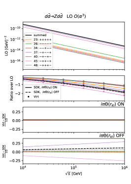
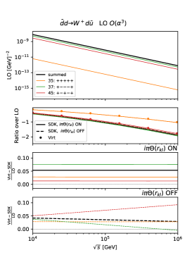
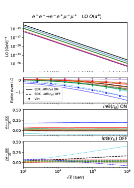
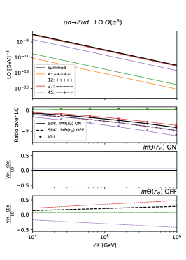
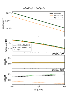
Figure 3: Comparison between exact results (dots) for ${\cal O}(\alpha)$ NLO EW virtual corrections and their LA (lines) in the case of squared matrix elements of representative $2\rightarrow n$ processes with $n=3,4$. Solid lines include the contributions proportional to $i\pi\Theta(r_{kl})$, while dashed lines do not. Plots show a scan in energy for fixed $r_{kl}/s$ ratios. More details are given in the text.

As explained in Sec. 2.2, in the original work of Ref. Denner:2000jv an imaginary component has been omitted in the formulas. On the other hand, this component affects results only for $2\rightarrow n$ processes with $n>2$. In this section we show numerical results about this aspect, for $2\rightarrow n$ partonic processes with $n=3,4$. Again, we select representative processes for which the relevant plots are displayed in Fig. 3. Each plot shows the dependence on $s$ of several quantities, and the layout is very similar to the one of the upper plots of Figs. 1 and 2. Here, the LA always includes the ${\SS^{s\rightarrow r_{kl}}}$ terms, but we distinguish the case in which the terms proportional to $i\pi\Theta(r_{kl})$ in eqs. (2.4)–(25) are excluded, as in the original DP algorithm in Ref. Denner:2000jv , or retained. The former are displayed as dashed lines ($i\pi\Theta(r_{kl})$ OFF) and the latter as solid lines ($i\pi\Theta(r_{kl})$ ON). For each leading helicity configuration, we also show in the second and third inset the difference between the LA and the exact result both normalised to the LO, respectively with and without taking into account the imaginary component.

In order to produce the plots, scanning in $\sqrt{s}$, we have performed a procedure similar to the one explained in the previous section for the upper plots in Figs. 1 and 2. The only difference here is the starting point. For $2\rightarrow n$ partonic processes with $n>2$, besides $s$, there is more than only one independent kinematic invariant that can be built with the external momenta. In order to avoid pathological configurations with an $|r_{kl}|\simeq M_{W}^{2}$, we randomly generate the first set of external momenta setting $\sqrt{s}=10^{4}~{}\,\textrm{GeV}$ and requiring

$$\frac{|r_{kl}|}{s}>\frac{1}{8}\qquad\forall~{}r_{kl}\,.$$ (88)

We remind the reader, as already explained in footnote 1, that eq. (88) is a condition that can be satisfied for $2\rightarrow 3$ or $2\rightarrow 4$ processes, but not in general for $2\rightarrow n$, for which this lower bound has to be lowered more and more increasing the value of $n$, further departing from the condition of eq. (4).

Looking at Fig. 3, it is manifest how the case including terms proportional to $i\pi\Theta(r_{kl})$ correctly catches the LA, while the other one does not; perfectly horizontal lines are present in the second inset, while in the third inset a dependence on $s$ is clearly visible. For some of the processes considered, such as $d\bar{d}\rightarrow Zd\bar{d}$, this dependence seems to cancel out for the sum over the different helicity configurations. In large part this is correct, but a small dependence is still present and it is simply not visible from the plot. We in general see this feature also for individual helicity configurations, namely the $i\pi\Theta(r_{kl})$ is often formally relevant but sometimes the numerical effect is very small. For other processes, such as $e^{+}e^{-}\rightarrow e^{+}e^{-}\mu^{+}\mu^{-}$ or $ud\rightarrow Zud$, even for the helicity-summed result the lack of the terms proportional to $i\pi\Theta(r_{kl})$ leads to sizeable numerical effects.

	$i\pi\Theta(r_{kl})$ ON		$i\pi\Theta(r_{kl})$ OFF
Helicity	$A$	$B$	$A$	$B$
summed	$(5\pm 28)\cdot 10^{-6}$	$(1.55\pm 0.01)\cdot 10^{-2}$	$(2.622\pm 0.004)\cdot 10^{-2}$	$(-4.00\pm 0.02)\cdot 10^{-2}$
$23:+++++$	$(1.3\pm 4.2)\cdot 10^{-6}$	$(1.318\pm 0.002)\cdot 10^{-2}$	$(-1.07\pm 0.02)\cdot 10^{-3}$	$(1.56\pm 0.01)\cdot 10^{-2}$
$26:-----$	$(2.2\pm 6.7)\cdot 10^{-6}$	$(1.380\pm 0.003)\cdot 10^{-2}$	$(-3.1\pm 0.2)\cdot 10^{-4}$	$(1.44\pm 0.01)\cdot 10^{-2}$
$34:--+--$	$(10\pm 10)\cdot 10^{-5}$	$(1.86\pm 0.05)\cdot 10^{-2}$	$(4.1\pm 0.8)\cdot 10^{-4}$	$(1.80\pm 0.04)\cdot 10^{-2}$
$37:-+--+$	$(2.7\pm 6.6)\cdot 10^{-5}$	$(6.4\pm 0.3)\cdot 10^{-3}$	$(7.408\pm 0.008)\cdot 10^{-2}$	$(-1.503\pm 0.004)\cdot 10^{-1}$
$40:-+-+-$	$(-8.0\pm 8.0)\cdot 10^{-5}$	$(2.24\pm 0.04)\cdot 10^{-2}$	$(-8.72\pm 0.09)\cdot 10^{-3}$	$(3.89\pm 0.04)\cdot 10^{-2}$
$45:-++-+$	$(-5\pm 50)\cdot 10^{-6}$	$(3.42\pm 0.02)\cdot 10^{-2}$	$(-7.405\pm 0.005)\cdot 10^{-2}$	$(1.909\pm 0.003)\cdot 10^{-1}$
$48:-+++-$	$(-5.2\pm 3.3)\cdot 10^{-6}$	$(2.901\pm 0.001)\cdot 10^{-2}$	$(8.631\pm 0.009)\cdot 10^{-3}$	$(1.251\pm 0.004)\cdot 10^{-2}$

Table 1: Result of the fit of the quantity (Virt-SDK)/LO using the method of least squares and the function (87) for the representative process $d\bar{d}\rightarrow Zd\bar{d}$ at ${\cal O}(\alpha^{3})$. The case including(excluding) the contribution of $i\pi\Theta(r_{kl})$ corresponds to the quantities shown in the second(third) inset of the upper-left plot of Fig. 3.

In order to provide a more quantitative statement, we list in Tab. 1 the results of the fit of (Virt-SDK)/LO for each leading-helicity configuration (and their sum) of the process $d\bar{d}\rightarrow Zd\bar{d}$. We have used again the method of least squares and the functional form of eq. (87). As can be seen in the third column of Tab. 1, all helicities exhibit a non-vanishing slope when the terms proportional to $i\pi\Theta(r_{kl})$ are turned off. Notably, as anticipated before, this happens also for the sum over the helicities, which for this particular process and kinematic configuration (condition (88)) leads to a cumulative error of $2.6\%$ in the LA for every factor of 10 in increase of the energy. The error is process dependent and can also be larger, as can be seen in the bottom-left plot of Fig. 3 for the $e^{+}e^{-}\rightarrow e^{+}e^{-}\mu^{+}\mu^{-}$ process.

Finally, given Fig. 3, we would like to stress how well the LA of Sudakov terms can work in the high-energy regime. All these processes receive corrections of the order of $-200\%$ and the difference between the LA and the exact result is always (well) below the $10\%$.

6.4 Impact of the corrections of QCD origin

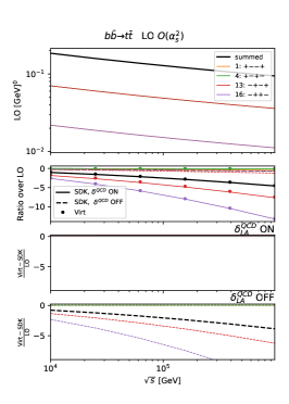
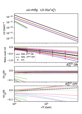
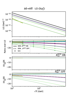
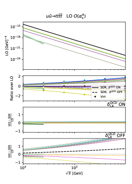
Figure 4: Comparison between exact results (dots) for ${\cal O}(\alpha)$ NLO EW virtual corrections and their LA (lines) in the case of squared matrix elements of representative $2\rightarrow n$ processes with $n=2,3,4$. Solid lines include the $\delta^{\rm QCD}_{\rm LA}$ contribution, while dashed lines do not. Plots show a scan in energy for fixed $r_{kl}/s$ ratios. More details are given in the text.

As explained in Sec. 3, NLO EW corrections can receive contribution of both EW and QCD origin (see discussion therein for details). In this section we show numerical results on this aspect, for $2\rightarrow n$ partonic processes with $n=2,3,4$. We again select representative processes for which the relevant plots are displayed in Figs. 4. Each plot shows the dependence on $s$ of several quantities, and the layout is very similar to the one of the plots of Fig. 3 in the previous section. Phase-space points have also been generated following the same procedure described in the previous section and according to the condition (88). As in Sec. 6.3 the LA always includes the ${\SS^{s\rightarrow r_{kl}}}$ terms in $\delta^{\rm EW}_{\rm LA}$, however here we distinguish the cases in which the term $\Sigma_{{\rm LO}_{i}}\delta^{\rm QCD}_{\rm LA}$ in eq. 51 is excluded or retained. The former are displayed as dashed lines (SDK, $\delta^{\rm QCD}_{\rm LA}$ OFF) and the latter as solid lines (SDK, $\delta^{\rm QCD}_{\rm LA}$ ON). For each leading helicity configuration, we also show in the second and third inset the difference between the LA and the exact result both normalised to the LO, respectively with and without taking into account the $\delta^{\rm QCD}_{\rm LA}$ component.

As can be seen in Fig. 4, perfectly horizontal lines are displayed only in the second inset. For each plot, lines in the third inset have a slope, which largely depends on the process considered. The slope is directly connected to the term $\Sigma_{{\rm LO}_{i}}\delta^{\rm QCD}_{\rm LA}$, therefore its size depends on both the size of $\delta^{\rm QCD}_{\rm LA}$ (see eq. (64)) and, since in the plots shown in Figs. 4 we have $i=2$, on the ${\rm LO}_{2}/{\rm LO}_{1}$ ratio.

Considering simple $2\rightarrow 2$ processes, one can see how different is the impact of $\Sigma_{{\rm LO}_{2}}\delta^{\rm QCD}_{\rm LA}$ in the top-left and top-center plots; in the case of $b\bar{b}\rightarrow t\bar{t}$ both $\delta^{\rm QCD}_{\rm LA}$ and the ${\rm LO}_{2}/{\rm LO}_{1}$ ratio are larger. The top-right plot refers to the process $u\bar{u}\rightarrow t\bar{t}gh$, the simplest process for which all the terms of eq. (64) are non-vanishing. The lower plots refer to different partonic processes entering the process $pp\rightarrow t\bar{t}t\bar{t}$. As already discussed in Ref. Frederix:2017wme a large part of the NLO EW corrections are of QCD origin, and this can be observed also in the lower plots of Fig. 4.

Given the large number of leading helicity configurations for processes with $t\bar{t}t\bar{t}$ in the final state, we did not list them in the legend of the corresponding plots of Fig. 4. On the other hand, in Tab. 2 we provide, as an example, the results of the fit of (Virt-SDK)/LO for all leading-helicity configurations (and their sum) for the process $gg\rightarrow t\bar{t}t\bar{t}$. We have used again the method of least squares and the function (87) as done for Tab. 1, but in this case we have considered two different scenarios: the inclusion or the exclusion of the $\delta^{\rm QCD}_{\rm LA}$ contribution. By comparing the numbers in the first and third column of Tab. 2, one can further see how the $\delta^{\rm QCD}_{\rm LA}$ contribution is essential in flattening the (Virt-SDK)/LO curve.

	$\delta^{\rm QCD}_{\rm LA}$ ON		$\delta^{\rm QCD}_{\rm LA}$ OFF
Helicity	$A$	$B$	$A$	$B$
summed	$(9.9\pm 8.4)\cdot 10^{-4}$	$(-2.7\pm 0.4)\cdot 10^{-2}$	$(-8.9\pm 1.2)\cdot 10^{-1}$	$(3.1\pm 0.6)\cdot 10^{0}$
$1:----++$	$(2.7\pm 1.6)\cdot 10^{-4}$	$(-2.56\pm 0.08)\cdot 10^{-2}$	$(-2.9\pm 0.4)\cdot 10^{-1}$	$(9.9\pm 1.8)\cdot 10^{-1}$
$6:---++-$	$(-5.5\pm 5.4)\cdot 10^{-3}$	$(6.6\pm 2.7)\cdot 10^{-2}$	$(5.3\pm 0.7)\cdot 10^{-1}$	$(-1.8\pm 0.4)\cdot 10^{0}$
$7:---+-+$	$(4.3\pm 6.7)\cdot 10^{-4}$	$(5.8\pm 0.3)\cdot 10^{-2}$	$(5.3\pm 0.7)\cdot 10^{-1}$	$(-1.8\pm 0.3)\cdot 10^{0}$
$10:--+-+-$	$(6.5\pm 6.1)\cdot 10^{-4}$	$(5.3\pm 0.3)\cdot 10^{-2}$	$(5.3\pm 0.7)\cdot 10^{-1}$	$(-1.8\pm 0.3)\cdot 10^{0}$
$11:--+--+$	$(-5.9\pm 5.8)\cdot 10^{-3}$	$(8.2\pm 2.9)\cdot 10^{-2}$	$(5.3\pm 0.7)\cdot 10^{-1}$	$(-1.8\pm 0.4)\cdot 10^{0}$
$16:--++--$	$(5\pm 14)\cdot 10^{-5}$	$(3.53\pm 0.07)\cdot 10^{-2}$	$(-1.4\pm 0.2)\cdot 10^{-1}$	$(5.4\pm 0.9)\cdot 10^{-1}$
$17:-+--++$	$(4.3\pm 6.3)\cdot 10^{-4}$	$(-4.6\pm 0.3)\cdot 10^{-2}$	$(-2.2\pm 0.3)\cdot 10^{-1}$	$(7.3\pm 1.4)\cdot 10^{-1}$
$22:-+-++-$	$(-5.5\pm 3.5)\cdot 10^{-4}$	$(-6.4\pm 0.2)\cdot 10^{-2}$	$(-2.3\pm 0.3)\cdot 10^{0}$	$(8.1\pm 1.5)\cdot 10^{0}$
$23:-+-+-+$	$(1.2\pm 0.6)\cdot 10^{-3}$	$(-6.3\pm 0.3)\cdot 10^{-2}$	$(-1.9\pm 0.3)\cdot 10^{0}$	$(6.9\pm 1.3)\cdot 10^{0}$
$26:-++-+-$	$(1.2\pm 0.9)\cdot 10^{-3}$	$(-5.9\pm 0.4)\cdot 10^{-2}$	$(-2.3\pm 0.3)\cdot 10^{0}$	$(8.2\pm 1.5)\cdot 10^{0}$
$27:-++--+$	$(-3.7\pm 5.0)\cdot 10^{-4}$	$(-8.1\pm 0.3)\cdot 10^{-2}$	$(-2.0\pm 0.3)\cdot 10^{0}$	$(7.0\pm 1.3)\cdot 10^{0}$
$32:-+++--$	$(3.1\pm 3.1)\cdot 10^{-4}$	$(2.7\pm 0.2)\cdot 10^{-2}$	$(-1.1\pm 0.1)\cdot 10^{-1}$	$(4.1\pm 0.6)\cdot 10^{-1}$
$33:+---++$	$(1.5\pm 1.2)\cdot 10^{-3}$	$(-4.5\pm 0.6)\cdot 10^{-2}$	$(-2.2\pm 0.3)\cdot 10^{-1}$	$(7.3\pm 1.4)\cdot 10^{-1}$
$38:+--++-$	$(1.4\pm 1.0)\cdot 10^{-3}$	$(-7.1\pm 0.5)\cdot 10^{-2}$	$(-2.0\pm 0.3)\cdot 10^{0}$	$(7.0\pm 1.3)\cdot 10^{0}$
$39:+--+-+$	$(-1.9\pm 3.7)\cdot 10^{-4}$	$(-7.4\pm 0.2)\cdot 10^{-2}$	$(-2.3\pm 0.3)\cdot 10^{0}$	$(8.2\pm 1.5)\cdot 10^{0}$
$42:+-+-+-$	$(-2.7\pm 2.5)\cdot 10^{-4}$	$(-8.3\pm 0.1)\cdot 10^{-2}$	$(-2.0\pm 0.3)\cdot 10^{0}$	$(6.8\pm 1.3)\cdot 10^{0}$
$43:+-+--+$	$(1.5\pm 0.7)\cdot 10^{-3}$	$(-6.6\pm 0.4)\cdot 10^{-2}$	$(-2.3\pm 0.3)\cdot 10^{0}$	$(8.1\pm 1.5)\cdot 10^{0}$
$48:+-++--$	$(4.0\pm 2.3)\cdot 10^{-4}$	$(2.1\pm 0.1)\cdot 10^{-2}$	$(-1.1\pm 0.1)\cdot 10^{-1}$	$(4.1\pm 0.6)\cdot 10^{-1}$
$49:++--++$	$(4.0\pm 2.5)\cdot 10^{-4}$	$(-2.9\pm 0.1)\cdot 10^{-2}$	$(-2.9\pm 0.4)\cdot 10^{-1}$	$(9.9\pm 1.8)\cdot 10^{-1}$
$54:++-++-$	$(7.4\pm 7.8)\cdot 10^{-4}$	$(4.9\pm 0.4)\cdot 10^{-2}$	$(5.3\pm 0.7)\cdot 10^{-1}$	$(-1.8\pm 0.3)\cdot 10^{0}$
$55:++-+-+$	$(-5.4\pm 5.2)\cdot 10^{-3}$	$(7.4\pm 2.6)\cdot 10^{-2}$	$(5.3\pm 0.7)\cdot 10^{-1}$	$(-1.8\pm 0.4)\cdot 10^{0}$
$58:+++-+-$	$(-6.0\pm 6.0)\cdot 10^{-3}$	$(7.7\pm 3.0)\cdot 10^{-2}$	$(5.3\pm 0.7)\cdot 10^{-1}$	$(-1.8\pm 0.4)\cdot 10^{0}$
$59:+++--+$	$(3.7\pm 4.6)\cdot 10^{-4}$	$(6.1\pm 0.2)\cdot 10^{-2}$	$(5.3\pm 0.7)\cdot 10^{-1}$	$(-1.8\pm 0.3)\cdot 10^{0}$
$64:++++--$	$(10\pm 141)\cdot 10^{-6}$	$(3.85\pm 0.07)\cdot 10^{-2}$	$(-1.4\pm 0.2)\cdot 10^{-1}$	$(5.4\pm 0.9)\cdot 10^{-1}$

Table 2: Result of the fit of the quantity (Virt-SDK)/LO using the method of least squares and the function (87) for the representative process $gg\rightarrow t\bar{t}t\bar{t}$. The case including(excluding) the $\delta^{\rm QCD}_{\rm LA}$ contribution corresponds to the quantities shown in the second(third) inset of the lower-central plot of Fig. 4.

7 Numerical Results: differential cross sections

In this section we consider IR-safe collider observables and we compare exact NLO EW predictions and their LA (the approximation given by Sudakov logarithms) obtained via the DP algorithm as framed in Sec. 4, i.e., the ${\rm SDK_{weak}}$ approach. We show differential distributions for proton–proton collisions at 100 TeV, which is one of the possible experimental set-ups that has been considered as an option for a high-energy future colliders Arkani-Hamed:2015vfh ; Mangano:2016jyj ; Contino:2016spe ; Dainese:2016gch . In this regime, LA is expected to be very efficient in capturing NLO EW effects. By explicit examples, we show how both the inclusion of the $\SS^{s\rightarrow r_{kl}}$ terms in eq. (17), which are relevant when the condition (4) is not satisfied, and the usage of the purely weak LA described in Sec. 4, the ${\rm SDK_{weak}}$ approach, has to be in general preferred for predictions of physical observables. Indeed, these features not only improve the LA, but they are also instrumental in order to capture the correct logarithmic dependence.

As already said, we consider cross-section predictions for differential distributions of IR-safe observables. Thus, bare leptons, which are treated as massless, have to be recombined with photons into dressed leptons. A dressed lepton is here obtained by recombining a bare lepton $\ell$ with any photon $\gamma$ that satisfies the condition

$$\Delta R(\ell,\gamma)<0.4\,,$$ (89)

where $\Delta R(\ell,\gamma)\equiv\sqrt{(\Delta\eta(\ell,\gamma))^{2}+(\Delta\phi(\ell,\gamma))^{2}}$, and $\Delta\eta(\ell,\gamma)$ and $\Delta\phi(\ell,\gamma)$ are the differences of the bare-lepton and photon pseudo-rapidities and azimuthal angles, respectively.

In this context, however, we recombine with photons any electrically charged particle, including top quarks and $W$ bosons, which are massive. This choice is not due to IR safety, but rather to the fact that very energetic massive particles are typically identified as tagged jets, namely a jet which contains the considered particle. The recombination of photons and heavy charged particles is inspired by precisely this procedure, and similarly the condition (89) leading to a large cone. In one case we will also consider the aforementioned tagged jets, where the clustering is performed not only with photons but with all the particles and afterwards tagging the considered heavy particle among the jet constituents. In that case, we will use the anti-$k_{T}$ algorithm Cacciari:2008gp as implemented in FastJet Cacciari:2011ma , with $R=0.4$. We remind the reader that, as already explained in Sec. 4.1, photon recombination has an effect on the LA: it cancels the virtual QED contributions associated to the collinear configuration in the final state, which is precisely what is taken into account by the ${\rm SDK_{weak}}$ approach.

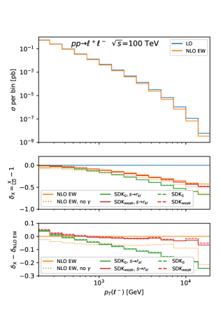
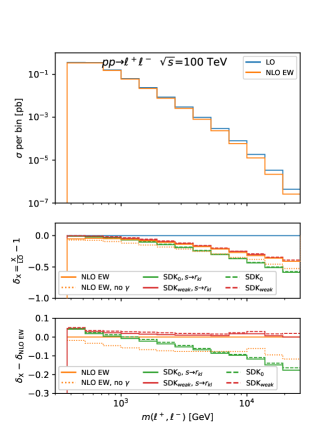
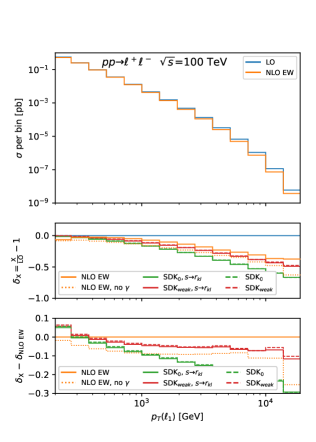
Figure 5: Differential distributions for recombined leptons in Drell-Yan production at 100 TeV. Comparison between exact NLO EW predictions (solid orange) and their LA approximations in the ${\rm SDK_{weak}}$ (red) and ${\rm SDK_{0}}$ (green) approaches, including (solid) or excluding (dashed) the $\SS^{s\rightarrow r_{kl}}$ terms. More details are given in the text.

7.1 Drell-Yan

We start discussing the case of Drell-Yan production with leptons in the final state, namely the process $pp\rightarrow\ell^{+}\ell^{-}$. For all processes that will be considered in this section we have used the same input parameters already listed in Sec. 6.1. However, in the case of Drell-Yan, we have employed the complex-mass scheme Denner:1999gp ; Denner:2005fg ; Frederix:2018nkq for the exact NLO EW corrections. We use the PDF set NNPDF3.1 Ball:2017nwa ; Bertone:2017bme , in particular the NNPDF31_nlo_as_0118_luxqed distributions, which include NLO QED evolution and especially a photon density following the LUXqed parameterisation Manohar:2016nzj ; Manohar:2017eqh . The renormalisation ($\mu_{R}$) and factorisation ($\mu_{F}$) scales are both set equal to the partonic center-of-mass energy $\sqrt{s}$. This set-up is common with all the other processes discussed in this section.

In the Drell-Yan simulation the following cuts are imposed on the dressed leptons:

$$p_{T}(\ell^{\pm})>200~{}\,\textrm{GeV}\,,\qquad|\eta(\ell^{\pm})|<2.5\,,\qquad m(\ell^{+},\ell^{-})>400~{}\,\textrm{GeV}\,,\qquad\Delta R(\ell^{+},\ell^{-})>0.5\,.$$ (90)

On the one hand, these cuts are imposed in order to resemble realistic experimental cuts for high-energy objects. On the other hand, they avoid additional logarithmic enhancements from collinear splittings appearing in the real radiation processes or even at the Born level. In Fig. 5 we show differential distributions for the transverse momentum of the electron, $p_{T}(\ell^{-})$, for the transverse momentum of the leading (trailing) lepton, $p_{T}(\ell_{1})$ ($p_{T}(\ell_{2})$), and for the dilepton invariant mass $m(\ell^{+},\ell^{-})$.

The layout of each plot in Fig. 5, and in general of each plot in this section, is the following. In the main panel we show the differential distribution at LO (solid blue line) and NLO EW (solid orange line) accuracy, where the exact ${\cal O}(\alpha)$ corrections are taken into account. If the NLO EW prediction turns negative, meaning that NLO EW corrections are negative and larger than the LO in absolute value, the curve corresponds to its absolute value and is drawn as dashed. In the first inset we show the relative impact of EW corrections, $\delta_{X}\equiv{X/{\rm LO}-1}$, in different approximations. The solid orange line corresponds to the one in the main panel with the same style, i.e. the exact ${\cal O}(\alpha)$ corrections (NLO EW), and the dotted orange line corresponds to the same case where the photon PDF has been set equal to zero (NLO EW, no $\gamma$). The other curves correspond to results in LA, with different assumptions. First, the solid curves include the $\SS^{s\rightarrow r_{kl}}$ contribution (${\rm SDK}_{X},s\rightarrow r_{kl}$), while the dashed ones do not (${\rm SDK}_{X}$). Second, the green lines are obtained by simply omitting the QED and IR-sensitive terms, which are dubbed as “em” in the DP algorithm. This is analogous to the approach of e.g. Refs. Chiesa:2013yma ; Bothmann:2020sxm and dubbed here as $\rm SDK_{0}$. The red lines are instead obtained by completely removing the QED contribution, namely, following the procedure described in Sec. 4.1, the $\rm SDK_{weak}$ approach. Both the $\rm SDK_{0}$ and $\rm SDK_{weak}$ predictions, similarly to the NLO EW ones in this section, include also the LO contribution. Needless to say, the closest a line is to the solid orange one, the better is the approximation of the exact NLO EW corrections. Therefore, in order to better judge this characteristic, in the second inset we zoom on the lines by simply plotting for each line in the first inset the difference with the solid orange one. Clearly, the reference prediction in LA is the solid red line, which both includes the $\SS^{s\rightarrow r_{kl}}$ contribution and is obtained via the $\rm SDK_{weak}$ approach.

We remind the reader that neither the $\rm SDK_{0}$ nor the $\rm SDK_{weak}$ approach are equal to the approach dubbed as SDK in Sec. 6, which concerns the LA of the interference of Born amplitude and the IR-divergent virtual amplitude. The SDK prediction cannot be used for IR-safe observables. Moreover, the $\rm SDK_{0}$ approach, even when the $\SS^{s\rightarrow r_{kl}}$ contributions are not taken into account, is not exactly equal to the one used so far in the literature, since we do include also in this case the terms proportional to $i\pi\Theta(r_{kl})$. This is particularly relevant for Secs. 7.2 and 7.4, where $2\rightarrow 3$ processes are considered.

Starting from the top-left plot of Fig. 5, the $p_{T}(\ell^{-})$ distribution, we can see how sound is the LA in the high-energy limit. The distribution is spanning two orders of magnitude of $p_{T}(\ell^{-})$, from 200 GeV to 20 TeV, and NLO EW corrections reach $\sim-50\%$ in the tail. As can be seen in the second inset, the solid red line differs from the solid orange line by only a very few percents of the LO. The situation is opposite for the green solid line. In that case the difference with the solid orange line grows logarithmically with $p_{T}(\ell^{-})$ and reaches $\sim-20\%$ of the LO in the tail. This is a clear example of how the $\rm SDK_{weak}$ approach can be superior to the $\rm SDK_{0}$ one in the approximating the exact NLO EW corrections for IR-safe collider observables. For this observable the differences between dashed and solid lines of the same colour are negligible. This is not surprising, since large $p_{T}(\ell^{-})$ implies large values of $t$ and therefore $|t|/s\sim{\cal O}(1)$, leading to small contributions from the $\SS^{s\rightarrow r_{kl}}$ terms. Finally, by looking at the difference between the solid and dotted orange line, we can also appreciate how the photon-initiated processes are relevant for this process and especially unavoidable also in the LA approximation in order to correctly approximate the exact NLO EW effects.

Moving to the top-right plot of Fig. 5, the $m(\ell^{+},\ell^{-})$ distribution, we see a very similar situation to the $p_{T}(\ell^{-})$ distribution. In this case there is a visible difference between solid and dashed lines of the same colours, with the solid red line better approximating the exact NLO EW result than the dashed red line. Indeed, large $m(\ell^{+},\ell^{-})$ values do not imply large values for $|t|$. However, due to the cuts in (90) the effect of the $\rm SDK_{weak}$ terms is very mild and also the dashed red line is leading to a very good approximation. The lower plots, the $p_{T}(\ell_{1})$ (left) and $p_{T}(\ell_{2})$ (right) distributions, display some differences w.r.t. the upper ones. For these two observable the LA is less efficient, indeed, as can be seen in the plots, the difference with the exact results can reach up to 5% of the LO also for solid red lines. However, this difference is converging to a constant value in the tail, for both distributions. Moreover the difference is of opposite sign for the two complementary observables, $p_{T}(\ell_{1})$ and $p_{T}(\ell_{2})$. This behaviour is due to the indirect cut that is affecting the recoiling particle when a particular value of $p_{T}(\ell_{1})$ or $p_{T}(\ell_{2})$ is considered, namely the trivial condition $p_{T}(\ell_{1})>p_{T}(\ell_{2})$. This has nothing to do with EW Sudakov effects, but it is a particular feature of this kind observables: a similar pattern was observed for top-quark pair production in Ref. Czakon:2019bcq . Indeed, we also verified this explicitly for top-quark pair production, which we do not show here since results are very similar to the case of Drell-Yan that we are discussing. The bottom line is that the $\rm SDK_{weak}$ approach including $\SS^{s\rightarrow r_{kl}}$ terms for LA can always have ${\cal O}(\alpha)$ finite discrepancies with the exact result, especially it cannot take into account effects that are not related to a Born-like kinematic. On the other hand, also for these two observables there are not logarithmically enhanced differences with the exact NLO EW prediction, only constant terms are present. Instead, with the $\rm SDK_{0}$ approach, the logarithmically enhanced differences are clearly visible.

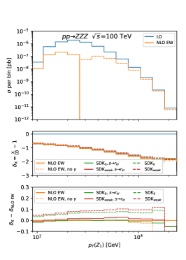
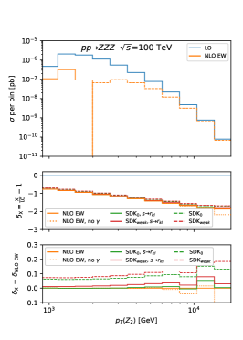
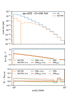
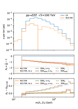
Figure 6: Same as Fig. 5, but for $ZZZ$ hadroproduction at 100 TeV.

7.2 ZZZ

In Fig. 6 we show plots, with the same layout of those in Fig. 5, for the process $pp\rightarrow ZZZ$. This process has a neutral final state, so we do not expect large differences between the $\rm SDK_{0}$ and $\rm SDK_{weak}$ approaches. On the other hand, being a $2\rightarrow 3$ process, the effect of the $\SS^{s\rightarrow r_{kl}}$ terms is supposed to be more relevant. The upper plots of Fig. 6 correspond to the transverse-momentum distributions of respectively the hardest $Z$-boson ($p_{T}(Z_{1})$), the second-hardest $Z$-boson ($p_{T}(Z_{2})$) and the softest one ($p_{T}(Z_{3})$). The lower plots instead correspond to the invariant masses $m(Z_{i},Z_{j})$ of the three different $Z$-boson pairs.

All the results have been obtained by applying the following cuts:

$$p_{T}(Z_{i})>1~{}\,\textrm{TeV}\,,\qquad|\eta(Z_{i})|<2.5\,,\qquad m(Z_{i},Z_{j})>1~{}\,\textrm{TeV}\,,\qquad\Delta R(Z_{i},Z_{j})>0.5\,.$$ (91)

Similarly to (90), these cuts resemble realistic experimental cuts for high-energy objects, but they also avoid additional logarithmic enhancements from collinear splittings appearing in the real-radiation processes or even at the Born.

First of all, it is important to notice the size of the EW corrections. For most of the spectrum of all distributions, they are negative and larger than the LO in absolute value, reaching $\sim-200\%$ of it in the tail. Since they are negative, this means that fixed-order NLO EW corrections are also negative in this regime and therefore non-physical. These distributions are a clear example of how large Sudakov logarithms, and in turn NLO EW corrections, can be at high energy. Also they clearly point to the necessity of resumming them in order to obtain sensible predictions. Here, on the other hand, we are not providing phenomenological predictions but rather showing the accuracy of the LA and testing its implementation in MadGraph5_aMC@NLO.

As expected, for all distributions, the difference between green and red lines ($\rm SDK_{0}$ and $\rm SDK_{weak}$) amounts to only few percents of the LO, with no clear logarithmic enhancement in the high-energy limit. Also as expected, the impact of the $\SS^{s\rightarrow r_{kl}}$ terms (solid versus dashed lines) is much larger for this process than for Drell-Yan production. In the upper plots of Fig. 5, the $p_{T}(Z_{i})$ distributions, the dashed lines are differing from the solid ones by 5-10% of the LO for the full spectra, with the latter in turn differing only by a very few percents from the exact NLO EW prediction. The difference between dashed and solid lines is even larger in the lower plots, the $m(Z_{i},Z_{j})$ distributions, and especially a clear logarithmic trend can be observed. It is worth to stress that for all these distributions, with the exception of the far tail in the $m(Z_{i},Z_{j})$ ones, the inclusion of the $\SS^{s\rightarrow r_{kl}}$ terms leads to an accuracy of very few percents for corrections spanning from $\sim$-80% to $\sim$-200%. This is not the case for the pure LA without the $\SS^{s\rightarrow r_{kl}}$ terms.

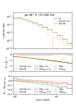
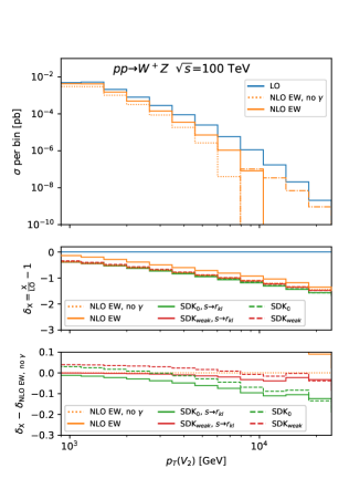
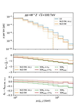
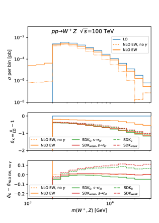
Figure 7: Differential distributions for recombined $V$ bosons in $W^{+}Z$ production at 100 TeV. Comparison between exact NLO EW predictions excluding photon-initiated processes (dotted orange) and their LA approximations in the ${\rm SDK_{weak}}$ (red) and ${\rm SDK_{0}}$ (green) approaches, including (solid) or excluding (dashed) the $\SS^{s\rightarrow r_{kl}}$ terms. More details are given in the text.

7.3 WZ

We now move to the case of a couple of processes where both the inclusion of the $\SS^{s\rightarrow r_{kl}}$ terms and the use of $\rm SDK_{weak}$ is relevant. We start by showing differential distributions for the process $pp\rightarrow W^{+}Z$, where results have been obtained by using the following cuts

$$p_{T}(V_{i})>1~{}\,\textrm{TeV}\,,\qquad|\eta(V_{i})|<2.5\,,\qquad m(W^{+},Z)>1~{}\,\textrm{TeV}\,,\qquad\Delta R(W^{+},Z)>0.5\,.$$ (92)

Again, these cuts resemble realistic experimental cuts for high-energy objects, but they also avoid (part of the) additional logarithmic enhancements from collinear splittings appearing in the real-radiation processes or even at the Born.

In Fig. 7 we show the transverse momentum of the hardest ($p_{T}(V_{1})$) and softest ($p_{T}(V_{2})$) recombined vector-bosons and their invariant mass ($m(W^{+},Z)$). Similarly to the case of leptons (89), the recombination is performed by recombining any charged vector boson $V_{i}$ with photons that satisfy the condition $\Delta R(V_{i},\gamma)<0.4$. We also show the transverse momentum ($p_{T}(j_{V,2})$) of the softest jet that is tagged as a $V$-jet, namely containing one of the two vector bosons. They layout of the plots is very similar to the ones of Figs. 5 and 6, but with an important difference: in the second inset we plot for each line in the first inset the difference with the dotted orange one, i.e., the exact NLO EW prediction where the photon PDF has been set equal to zero. The reason is the following. The $WZ$ production is affected by giant $K$-factors not only at NLO QCD Frixione:1992pj ; Frixione:1993yp , but also at NLO EW Baglio:2013toa ; Mangano:2016jyj precisely due to the opening of the $q\gamma\rightarrow W^{+}Zq^{\prime}$ channel. For large value of $p_{T}(V_{1})$ this channel induces large positive corrections of order $L(p_{T}^{2}(V_{1}),M^{2}_{V_{2}})$, due to configurations in which $V_{1}$ recoils against the emitted quark $q^{\prime}$ and $V_{2}$ is soft and collinear to it. This effect has nothing to do with virtual NLO EW corrections and cannot be expected to be captured by the DP algorithm, both in its $\rm SDK_{0}$ and $\rm SDK_{weak}$ adaptations for physical observables. Therefore, in order to test the LA, we use as reference the NLO EW prediction where the photon PDF has been set equal to zero. We also plot in the main panel the NLO EW prediction without photon PDF as dotted orange line and its absolute value as dashed-dotted when it becomes negative. We remind the reader that the photon PDF is entering the process starting with NLO EW real emission of quarks, while it is not present at LO.

Before commenting each plot of Fig. 7, it is again important to note how LA in general approximates very well the exact NLO EW predictions excluding photon-initiated processes, reaching almost -200% of the LO in the tail of the distributions. This can be appreciated in the first inset of each plot. There, as in the main panel, the size of the $q\gamma\rightarrow W^{+}Zq^{\prime}$ channel can also be appreciated. Its impact is maximal in the $p_{T}(V_{1})$ distribution, due to the aforementioned $L(p_{T}^{2}(V_{1}),M^{2}_{V_{2}})$ enhancement, and minimal in the $p_{T}(V_{2})$ distribution since large values of $p_{T}(V_{2})$ forbid the kinematic configurations that precisely lead to the enhancement for the $p_{T}(V_{1})$ distribution.

In the top-left plot ($p_{T}(V_{1})$) we can see that none of the curves is really flat. This is not surprising, since the LA works very well when the cross section is dominated by the Born-like kinematic, which is not the case for large $p_{T}(V_{1})$, where $V_{1}$ can in principle recoil against a very hard photon. Still, the solid red line ($\rm SDK_{weak}$ with $\SS^{s\rightarrow r_{kl}}$ terms included) leads to the best approximation and differs from the reference value, the dotted orange line, by less than 10% of the LO also in regions where the NLO EW corrections are $\sim-200\%$. The superiority of the $\rm SDK_{weak}$ approach (red) over the $\rm SDK_{0}$ one (green) and of the inclusion of the $\SS^{s\rightarrow r_{kl}}$ terms (solid) over their exclusion (dashed) can be better appreciated in the top-right plot ($p_{T}(V_{2})$) and especially in the bottom-right one $m(W^{+},Z)$. The difference between the dotted orange and solid red curves is only very few percents of the LO over the full range.

In the bottom-left plot, the $p_{T}(j_{V,2})$ distributions, all the curves are equal to those of the top-right one $p_{T}(V_{2})$ but one: the solid orange line. In this context the only difference between a recombined $V$-boson and a $V$-tagged jet is that in the latter the $V$ boson can be recombined also with quarks. When the $q\gamma\rightarrow W^{+}Zq^{\prime}$ channel is included, soft+collinear configurations for $(V_{2})$ in the final-state splitting $q^{(\prime)}\rightarrow q^{\prime}V_{2}$ are avoided at large $p_{T}(V_{2})$, but the purely collinear ones still survive. The recombination of $V_{2}$ with quarks has therefore a sizeable impact. The bottom line is that the $\rm SDK_{weak}$ approach takes into account only those emissions that are unavoidable from an IR-safety point of view, but additional real-emission contributions can be present and sizeable (for instance the photon-induced quark radiation), they can lead to enhancements factorising different Born matrix elements (for instance the case discussed here where $\sigma(q\gamma\rightarrow W^{+}Zq^{\prime})\propto\sigma(q\gamma\rightarrow W^{+}q^{\prime})\times L(p_{T}^{2}(W^{+}),M_{Z}^{2})$ or $\sigma(q\gamma\rightarrow W^{+}Zq^{\prime})\propto\sigma(q\gamma\rightarrow Zq)\times L(p_{T}^{2}(Z),M_{W}^{2})$) and their impact can depend on how the different particles are clustered among each other (for instance $V$-bosons versus $V$-tagged jet). These contributions cannot be taken into account via the DP algorithm. The LA and in particular the DP algorithm as implemented in MadGraph5_aMC@NLO allow for a fast and, as shown in the previous examples, very reliable approximation of fixed-order exact NLO EW corrections. On the other hand, it cannot substitute the exact calculation. LA can be used as a starting point for improving the fixed-order NLO EW, by e.g. resumming the large Sudakov logarithms or alternatively for performing fast simulations with MadGraph5_aMC@NLO including the EW dominant effects at high-energy. The latter option, however, should be always cross-checked with an exact calculation before being used for phenomenological predictions.

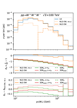
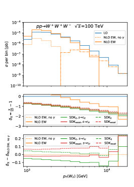
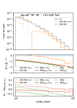
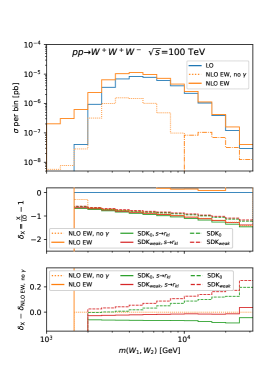
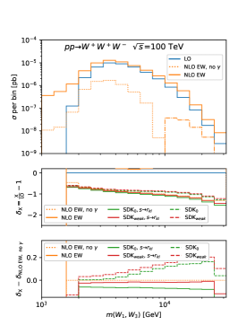
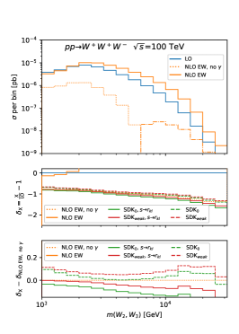
Figure 8: Same as Fig. 7, but for $W^{+}W^{+}W^{-}$ hadroproduction at 100 TeV.

7.4 WWW

As last example, we show in Fig. 8 distributions for the process $pp\rightarrow W^{+}W^{+}W^{-}$, where for the calculations the following cuts have been employed

$$p_{T}(W_{i})>1~{}\,\textrm{TeV}\,,\qquad|\eta(W_{i})|<2.5\,,\qquad m(W_{i},W_{j})>1~{}\,\textrm{TeV}\,,\qquad\Delta R(W_{i},W_{j})>0.5\,,$$ (93)

following the same rationale behind the cuts that have been used for the other processes considered in this section. In Fig. 8 we consider the same observables already considered in Fig. 6, with $Z$ bosons replaced by $W$ bosons. The layout of the plots is the same of those in Fig. 7 for $W^{+}Z$ production, where the reference line is the dotted orange one, the NLO EW prediction without photon-initiated processes. Indeed, also in this case the opening of the photon-induced channels in the NLO EW corrections ($q\gamma\rightarrow W^{+}W^{+}W^{-}q^{\prime}$) induces additional effects that cannot be captured by the DP algorithm.

Similarly to the case of $W^{+}Z$ production in Fig. 7, we see that both the choices between $\rm SDK_{0}$ and $\rm SDK_{weak}$ approaches and between the inclusion or exclusion of $\SS^{s\rightarrow r_{kl}}$ terms are relevant. Also, the exclusion of the photon-initiated processes is unavoidable for the comparison between LA and exact NLO EW results. As any other observable considered in this chapter, once again we see very large effects from NLO EW corrections (reaching almost $-200\%$ of the LO). Moreover, the solid red line, the LA in the $\rm SDK_{weak}$ approach including $\SS^{s\rightarrow r_{kl}}$ terms, is able to approximate within the 10% level the exact NLO EW effects excluding photon-initiated processes (dotted orange line) over the full range of the observables considered the plots of Fig. 8. The difference between the two aforementioned accuracies, the solid red line in the second inset, is in general a constant over the range of each observable considered. The only exception is $m(W_{2},W_{3})$ where a logarithmic trend is visible also for the red-solid line. A similar effect, although milder, could be observed also for the $m(Z_{2},Z_{3})$ distribution in $ZZZ$ production in Fig. 6. To the best of our knowledge, given the cuts in (93), this effect is not due to any possible enhancement arising from real emission contributions. However, as explained in Sec. 6, possible additional angular-dependent effects involving ratios of invariants can be present and not captured in the DP algorithm, regardless of the inclusion of the $\SS^{s\rightarrow r_{kl}}$ term.

8 Conclusions and outlook

In this work we have revisited the algorithm of Denner and Pozzorini Denner:2000jv for the calculation of one-loop EW Sudakov logarithms, denoted in the previous sections as DP algorithm. We have introduced several novelties that concern different aspects of the electroweak Sudakov approximation. Moreover, we have implemented the DP algorithm, together with the novelties introduced, in the MadGraph5_aMC@NLO framework. Thanks to this new implementation we have provided in a completely automated approach several numerical results for different production processes, both for the virtual contribution in specific phase-space points and for physical (IR-safe) differential cross sections at a 100 TeV proton–proton collider. All the numerical results that we have obtained corroborate the relevance of the novelties introduced in this work and also demonstrate the correctness of the implementation of the algorithm in the code.

In particular we have introduced the following novelties:

• We have reframed the DP algorithm by setting the mass of the photon and light-fermion masses exactly to zero, regularising IR divergences by mean of Dimensional Regularisation (DR), as in modern NLO EW calculations and Monte Carlo implementations. Reframing the algorithm with the language of modern calculations, it allows for further developments and compatibility with the state-of-the-art tool implementations.

• We have modified part of the expressions in order to take into account additional angular dependences, without assuming that all the invariants are of the same size of $s$. These modifications correspond to the terms that have been dubbed in the work as $\SS^{s\rightarrow r_{kl}}$; they have been obtained keeping track of the dependence on any invariant $r_{kl}$ in the derivation of the subleading soft-collinear logarithms. As already mentioned in various points in the text, even with this improvement, the full control of logarithms involving the ratios of the different $|r_{kl}|$ and $s$ cannot be achieved via the DP algorithm. Information on the internal structure of the diagrams is unavoidable for this purpose. On the other hand, the $\SS^{s\rightarrow r_{kl}}$ terms are sensitive to the presence of a hierarchy among the various invariants that characterise a specific phase-space point and substantially improve the approximation of the aforementioned class of logarithms. In order to support this statement, we have showcased for several processes and observables the superiority of the Sudakov approximation including the $\SS^{s\rightarrow r_{kl}}$ terms.

• We have identified an imaginary term that was omitted in Ref. Denner:2000jv , which cannot be in general neglected for $2\rightarrow n$ processes with $n>2$. This term is also present in the new $\SS^{s\rightarrow r_{kl}}$ terms that have been introduced. We have shown the relevance of this imaginary term for correctly capturing effects of order $\alpha\log(s/M_{W}^{2})$.

• In this work we did not focus only on one-loop EW corrections to amplitudes, as done in the pioneering work Ref. Denner:2000jv , but we have considered also the virtual NLO EW corrections to the LO cross sections. The two cases are trivially related only when the entire LO factorises a single combination of $\alpha_{\scriptscriptstyle S}$ and $\alpha$ powers. However, more in general, NLO EW corrections can also include effects due to loops of QCD origin. We provide the additional terms, denoted in the paper as $\delta^{\rm QCD}_{\rm LA}$, that are necessary in order to take into account in Sudakov approximation also contributions from the aforementioned QCD loops. We have proved the relevance of $\delta^{\rm QCD}_{\rm LA}$ for correctly capturing effects of order $\alpha\log^{n}(s/M_{W}^{2})$ with $n=1,2$, when also QCD loops contribute to virtual NLO EW corrections to the LO cross sections.

• We describe how to modify the DP algorithm in order to exclude the contribution of photons and also the contribution of gluons from the QCD terms mentioned in the previous bullet. We dub this approach as $\rm SDK_{weak}$. In the context of differential cross sections and IR physical observables, we show how this approach is superior to the standard approach used in the literature, dubbed in this work as $\rm SDK_{0}$, which corresponds to simply removing the IR-divergent logarithms involving the scale $M_{W}$ and the IR cut-off.

We discuss also the technical steps of the implementation of the DP algorithm, together with the novelties introduced in this work, in the MadGraph5_aMC@NLO framework. The choice of the MadGraph5_aMC@NLO framework, which already automates the calculation of the exact NLO EW corrections, has been crucial for the validation of our work and for demonstrating the correctness of our implementation of the Sudakov approximation, also denoted in the paper as leading approximation (LA). Systematic comparisons between exact ${\cal O}(\alpha)$ corrections, the NLO EW, and their LA with different assumptions ($\SS^{s\rightarrow r_{kl}}$, imaginary term, $\delta^{\rm QCD}_{\rm LA}$, $\rm SDK_{weak}$, etc.) have been performed in order to check that all the logarithmic terms are correctly captured.

Besides being essential for validation, the implementation in a framework as MadGraph5_aMC@NLO opens up for several new possibilities. First of all, the necessary ingredients for performing completely automated NLO EW corrections matched with resummed EW Sudakov logarithms are now available in a single tool. Then, a fast and stable method for approximating dominant effects from EW corrections is now available. Especially, the quality of the approximation can be checked via the NLO EW exact calculation, which however we remind the reader cannot in general be substituted by its LA. Sudakov effects can be also more easily integrated in Monte Carlo simulations and generations of events. These are only a few of the possible outcomes of this work, which sets the basis for future works both at the phenomenological and formal level.

Another important possible development of this work is, e.g., the possibility of compute approximate EW corrections also in extensions of the SM. Indeed, only tree-level Feynman rules are needed. However, for a given BSM model, the associated Universal Feynrules Output (UFO) model Degrande:2011ua , which is the format used in MadGraph5_aMC@NLO for encoding the Feynman rules, should provide some extra informations that are not present at the moment: how particles are arranged in SU(2) multiplets and the values of their electroweak couplings (charge, isospin component and/or hypercharge). At the moment, this information had to be written by hand in the code. We thus envisage an extension of the UFO format in this direction.

As a final remark, we want to stress once again that the Sudakov approximation cannot substitute exact NLO EW calculations. As we said, this approximation can be exploited for performing fast simulations including the EW dominant effects at high energy. However, it should be always cross-checked with an exact calculation before being used for phenomenological predictions and especially comparisons with data. Moreover, as explained many times in the text, the approximation works when all the invariants $r_{kl}$ satisfy the relation $|r_{kl}|\gg M_{W}^{2}$. This implies, for instance, that the Sudakov approximation can never be directly exploited for a process involving resonances. In the SM this typically means the production and decay of the heavy particles $W,Z,H$ or $t$. On the other hand, given such a type of process, the Sudakov approximation can be applied for the calculation of the same process including only the production but not the decays of the aforementioned heavy particles, and the decay can be subsequently taken into account.

References

- (1) ATLAS collaboration, G. Aad et al., Observation of a new particle in the search for the Standard Model Higgs boson with the ATLAS detector at the LHC, Phys. Lett. B 716 (2012) 1–29, [1207.7214].
- (2) CMS collaboration, S. Chatrchyan et al., Observation of a New Boson at a Mass of 125 GeV with the CMS Experiment at the LHC, Phys. Lett. B 716 (2012) 30–61, [1207.7235].
- (3) ATLAS collaboration, G. Aad et al., Combined measurements of Higgs boson production and decay using up to fb-1 of proton-proton collision data at 13 TeV collected with the ATLAS experiment, Phys. Rev. D 101 (2020) 012002, [1909.02845].
- (4) P. Azzi et al., Report from Working Group 1: Standard Model Physics at the HL-LHC and HE-LHC, CERN Yellow Rep. Monogr. 7 (2019) 1–220, [1902.04070].
- (5) M. Cepeda et al., Report from Working Group 2: Higgs Physics at the HL-LHC and HE-LHC, CERN Yellow Rep. Monogr. 7 (2019) 221–584, [1902.00134].
- (6) X. Cid Vidal et al., Report from Working Group 3: Beyond the Standard Model physics at the HL-LHC and HE-LHC, CERN Yellow Rep. Monogr. 7 (2019) 585–865, [1812.07831].
- (7) A. Cerri et al., Report from Working Group 4: Opportunities in Flavour Physics at the HL-LHC and HE-LHC, CERN Yellow Rep. Monogr. 7 (2019) 867–1158, [1812.07638].
- (8) Z. Citron et al., Report from Working Group 5: Future physics opportunities for high-density QCD at the LHC with heavy-ion and proton beams, CERN Yellow Rep. Monogr. 7 (2019) 1159–1410, [1812.06772].
- (9) E. Chapon et al., Perspectives for quarkonium studies at the high-luminosity LHC, 2012.14161.
- (10) H. M. Gray, Future colliders for the high-energy frontier, Rev. Phys. 6 (2021) 100053.
- (11) S. Kallweit, J. M. Lindert, P. Maierhöfer, S. Pozzorini and M. Schönherr, NLO electroweak automation and precise predictions for W+multijet production at the LHC, JHEP 04 (2015) 012, [1412.5157].
- (12) S. Frixione, V. Hirschi, D. Pagani, H. S. Shao and M. Zaro, Electroweak and QCD corrections to top-pair hadroproduction in association with heavy bosons, JHEP 06 (2015) 184, [1504.03446].
- (13) M. Chiesa, N. Greiner and F. Tramontano, Automation of electroweak corrections for LHC processes, J. Phys. G 43 (2016) 013002, [1507.08579].
- (14) B. Biedermann, S. Bräuer, A. Denner, M. Pellen, S. Schumann and J. M. Thompson, Automation of NLO QCD and EW corrections with Sherpa and Recola, Eur. Phys. J. C 77 (2017) 492, [1704.05783].
- (15) M. Chiesa, N. Greiner, M. Schönherr and F. Tramontano, Electroweak corrections to diphoton plus jets, JHEP 10 (2017) 181, [1706.09022].
- (16) R. Frederix, S. Frixione, V. Hirschi, D. Pagani, H. S. Shao and M. Zaro, The automation of next-to-leading order electroweak calculations, JHEP 07 (2018) 185, [1804.10017].
- (17) D. Pagani, H.-S. Shao, I. Tsinikos and M. Zaro, Automated EW corrections with isolated photons: , and as case studies, JHEP 09 (2021) 155, [2106.02059].
- (18) V. Hirschi, R. Frederix, S. Frixione, M. V. Garzelli, F. Maltoni and R. Pittau, Automation of one-loop QCD corrections, JHEP 05 (2011) 044, [1103.0621].
- (19) G. Cullen, N. Greiner, G. Heinrich, G. Luisoni, P. Mastrolia, G. Ossola et al., Automated One-Loop Calculations with GoSam, Eur. Phys. J. C 72 (2012) 1889, [1111.2034].
- (20) F. Cascioli, P. Maierhofer and S. Pozzorini, Scattering Amplitudes with Open Loops, Phys. Rev. Lett. 108 (2012) 111601, [1111.5206].
- (21) S. Actis, A. Denner, L. Hofer, A. Scharf and S. Uccirati, Recursive generation of one-loop amplitudes in the Standard Model, JHEP 04 (2013) 037, [1211.6316].
- (22) S. Actis, A. Denner, L. Hofer, J.-N. Lang, A. Scharf and S. Uccirati, RECOLA: REcursive Computation of One-Loop Amplitudes, Comput. Phys. Commun. 214 (2017) 140–173, [1605.01090].
- (23) A. Denner, J.-N. Lang and S. Uccirati, Recola2: REcursive Computation of One-Loop Amplitudes 2, Comput. Phys. Commun. 224 (2018) 346–361, [1711.07388].
- (24) F. Buccioni, J.-N. Lang, J. M. Lindert, P. Maierhöfer, S. Pozzorini, H. Zhang et al., OpenLoops 2, Eur. Phys. J. C 79 (2019) 866, [1907.13071].
- (25) V. V. Sudakov, Vertex parts at very high-energies in quantum electrodynamics, Sov. Phys. JETP 3 (1956) 65–71.
- (26) P. Ciafaloni and D. Comelli, Sudakov enhancement of electroweak corrections, Phys. Lett. B 446 (1999) 278–284, [hep-ph/9809321].
- (27) P. Ciafaloni and D. Comelli, Electroweak Sudakov form-factors and nonfactorizable soft QED effects at NLC energies, Phys. Lett. B 476 (2000) 49–57, [hep-ph/9910278].
- (28) M. Ciafaloni, P. Ciafaloni and D. Comelli, Bloch-Nordsieck violating electroweak corrections to inclusive TeV scale hard processes, Phys. Rev. Lett. 84 (2000) 4810–4813, [hep-ph/0001142].
- (29) A. Manohar, B. Shotwell, C. Bauer and S. Turczyk, Non-cancellation of electroweak logarithms in high-energy scattering, Phys. Lett. B 740 (2015) 179–187, [1409.1918].
- (30) M. Beccaria, G. Montagna, F. Piccinini, F. M. Renard and C. Verzegnassi, Rising bosonic electroweak virtual effects at high-energy e+ e- colliders, Phys. Rev. D 58 (1998) 093014, [hep-ph/9805250].
- (31) V. S. Fadin, L. N. Lipatov, A. D. Martin and M. Melles, Resummation of double logarithms in electroweak high-energy processes, Phys. Rev. D 61 (2000) 094002, [hep-ph/9910338].
- (32) M. Melles, Subleading Sudakov logarithms in electroweak high-energy processes to all orders, Phys. Rev. D 63 (2001) 034003, [hep-ph/0004056].
- (33) M. Melles, Mass gap effects and higher order electroweak Sudakov logarithms, Phys. Lett. B 495 (2000) 81–86, [hep-ph/0006077].
- (34) M. Melles, Resummation of Yukawa enhanced and subleading Sudakov logarithms in longitudinal gauge boson and Higgs production, Phys. Rev. D 64 (2001) 014011, [hep-ph/0012157].
- (35) M. Melles, Electroweak renormalization group corrections in high-energy processes, Phys. Rev. D 64 (2001) 054003, [hep-ph/0102097].
- (36) M. Melles, Electroweak radiative corrections in high-energy processes, Phys. Rept. 375 (2003) 219–326, [hep-ph/0104232].
- (37) M. Ciafaloni, P. Ciafaloni and D. Comelli, Electroweak Bloch-Nordsieck violation at the TeV scale: ’Strong’ weak interactions?, Nucl. Phys. B 589 (2000) 359–380, [hep-ph/0004071].
- (38) M. Ciafaloni, P. Ciafaloni and D. Comelli, Electroweak double logarithms in inclusive observables for a generic initial state, Phys. Lett. B 501 (2001) 216–222, [hep-ph/0007096].
- (39) A. Denner and S. Pozzorini, One loop leading logarithms in electroweak radiative corrections. 1. Results, Eur. Phys. J. C 18 (2001) 461–480, [hep-ph/0010201].
- (40) M. Melles, Resummation of angular dependent corrections in spontaneously broken gauge theories, Eur. Phys. J. C 24 (2002) 193–204, [hep-ph/0108221].
- (41) M. Ciafaloni, P. Ciafaloni and D. Comelli, Bloch-Nordsieck violation in spontaneously broken Abelian theories, Phys. Rev. Lett. 87 (2001) 211802, [hep-ph/0103315].
- (42) M. Ciafaloni, P. Ciafaloni and D. Comelli, Enhanced electroweak corrections to inclusive boson fusion processes at the TeV scale, Nucl. Phys. B 613 (2001) 382–406, [hep-ph/0103316].
- (43) A. Denner and S. Pozzorini, One loop leading logarithms in electroweak radiative corrections. 2. Factorization of collinear singularities, Eur. Phys. J. C 21 (2001) 63–79, [hep-ph/0104127].
- (44) A. Denner, M. Melles and S. Pozzorini, Two loop electroweak angular dependent logarithms at high-energies, Nucl. Phys. B 662 (2003) 299–333, [hep-ph/0301241].
- (45) A. Denner and S. Pozzorini, An Algorithm for the high-energy expansion of multi-loop diagrams to next-to-leading logarithmic accuracy, Nucl. Phys. B 717 (2005) 48–85, [hep-ph/0408068].
- (46) A. Denner, B. Jantzen and S. Pozzorini, Two-loop electroweak next-to-leading logarithmic corrections to massless fermionic processes, Nucl. Phys. B 761 (2007) 1–62, [hep-ph/0608326].
- (47) J.-y. Chiu, F. Golf, R. Kelley and A. V. Manohar, Electroweak Sudakov corrections using effective field theory, Phys. Rev. Lett. 100 (2008) 021802, [0709.2377].
- (48) J.-y. Chiu, F. Golf, R. Kelley and A. V. Manohar, Electroweak Corrections in High Energy Processes using Effective Field Theory, Phys. Rev. D 77 (2008) 053004, [0712.0396].
- (49) J.-y. Chiu, R. Kelley and A. V. Manohar, Electroweak Corrections using Effective Field Theory: Applications to the LHC, Phys. Rev. D 78 (2008) 073006, [0806.1240].
- (50) A. Denner, B. Jantzen and S. Pozzorini, Two-loop electroweak next-to-leading logarithms for processes involving heavy quarks, JHEP 11 (2008) 062, [0809.0800].
- (51) J.-y. Chiu, A. Fuhrer, R. Kelley and A. V. Manohar, Factorization Structure of Gauge Theory Amplitudes and Application to Hard Scattering Processes at the LHC, Phys. Rev. D 80 (2009) 094013, [0909.0012].
- (52) J. H. Kuhn, A. A. Penin and V. A. Smirnov, Summing up subleading Sudakov logarithms, Eur. Phys. J. C 17 (2000) 97–105, [hep-ph/9912503].
- (53) M. Beccaria, F. M. Renard and C. Verzegnassi, Top quark production at future lepton colliders in the asymptotic regime, Phys. Rev. D 63 (2001) 053013, [hep-ph/0010205].
- (54) M. Hori, H. Kawamura and J. Kodaira, Electroweak Sudakov at two loop level, Phys. Lett. B 491 (2000) 275–279, [hep-ph/0007329].
- (55) W. Beenakker and A. Werthenbach, Electroweak two loop Sudakov logarithms for on-shell fermions and bosons, Nucl. Phys. B 630 (2002) 3–54, [hep-ph/0112030].
- (56) S. Pozzorini, Next to leading mass singularities in two loop electroweak singlet form-factors, Nucl. Phys. B 692 (2004) 135–174, [hep-ph/0401087].
- (57) B. Feucht, J. H. Kuhn, A. A. Penin and V. A. Smirnov, Two loop Sudakov form-factor in a theory with mass gap, Phys. Rev. Lett. 93 (2004) 101802, [hep-ph/0404082].
- (58) B. Jantzen, J. H. Kuhn, A. A. Penin and V. A. Smirnov, Two-loop electroweak logarithms, Phys. Rev. D 72 (2005) 051301, [hep-ph/0504111].
- (59) B. Jantzen, J. H. Kuhn, A. A. Penin and V. A. Smirnov, Two-loop electroweak logarithms in four-fermion processes at high energy, Nucl. Phys. B 731 (2005) 188–212, [hep-ph/0509157].
- (60) B. Jantzen and V. A. Smirnov, The Two-loop vector form-factor in the Sudakov limit, Eur. Phys. J. C 47 (2006) 671–695, [hep-ph/0603133].
- (61) A. V. Manohar and M. Trott, Electroweak Sudakov Corrections and the Top Quark Forward-Backward Asymmetry, Phys. Lett. B 711 (2012) 313–316, [1201.3926].
- (62) C. W. Bauer, N. Ferland and B. R. Webber, Combining initial-state resummation with fixed-order calculations of electroweak corrections, JHEP 04 (2018) 125, [1712.07147].
- (63) A. V. Manohar and W. J. Waalewijn, Electroweak Logarithms in Inclusive Cross Sections, JHEP 08 (2018) 137, [1802.08687].
- (64) C. W. Bauer, S. Fleming and M. E. Luke, Summing Sudakov logarithms in B — X(s gamma) in effective field theory, Phys. Rev. D 63 (2000) 014006, [hep-ph/0005275].
- (65) C. W. Bauer, S. Fleming, D. Pirjol and I. W. Stewart, An Effective field theory for collinear and soft gluons: Heavy to light decays, Phys. Rev. D 63 (2001) 114020, [hep-ph/0011336].
- (66) C. W. Bauer and I. W. Stewart, Invariant operators in collinear effective theory, Phys. Lett. B 516 (2001) 134–142, [hep-ph/0107001].
- (67) C. W. Bauer, D. Pirjol and I. W. Stewart, Soft collinear factorization in effective field theory, Phys. Rev. D 65 (2002) 054022, [hep-ph/0109045].
- (68) M. Ciafaloni, P. Ciafaloni and D. Comelli, Towards collinear evolution equations in electroweak theory, Phys. Rev. Lett. 88 (2002) 102001, [hep-ph/0111109].
- (69) P. Ciafaloni, D. Comelli and A. Vergine, Sudakov electroweak effects in transversely polarized beams, JHEP 07 (2004) 039, [hep-ph/0311260].
- (70) P. Ciafaloni and D. Comelli, Electroweak evolution equations, JHEP 11 (2005) 022, [hep-ph/0505047].
- (71) P. Ciafaloni and D. Comelli, The Importance of weak bosons emission at LHC, JHEP 09 (2006) 055, [hep-ph/0604070].
- (72) M. Ciafaloni, P. Ciafaloni and D. Comelli, Electroweak double-logs at small x, JHEP 05 (2008) 039, [0802.0168].
- (73) G. Bell, J. H. Kuhn and J. Rittinger, Electroweak Sudakov Logarithms and Real Gauge-Boson Radiation in the TeV Region, Eur. Phys. J. C 70 (2010) 659–671, [1004.4117].
- (74) P. Ciafaloni, D. Comelli, A. Riotto, F. Sala, A. Strumia and A. Urbano, Weak Corrections are Relevant for Dark Matter Indirect Detection, JCAP 03 (2011) 019, [1009.0224].
- (75) W. J. Stirling and E. Vryonidou, Electroweak corrections and Bloch-Nordsieck violations in 2-to-2 processes at the LHC, JHEP 04 (2013) 155, [1212.6537].
- (76) C. W. Bauer and N. Ferland, Resummation of electroweak Sudakov logarithms for real radiation, JHEP 09 (2016) 025, [1601.07190].
- (77) U. Baur, Weak Boson Emission in Hadron Collider Processes, Phys. Rev. D 75 (2007) 013005, [hep-ph/0611241].
- (78) Z. Bern, G. Diana, L. J. Dixon, F. Febres Cordero, S. Höche, H. Ita et al., Missing Energy and Jets for Supersymmetry Searches, Phys. Rev. D 87 (2013) 034026, [1206.6064].
- (79) M. Chiesa, G. Montagna, L. Barzè, M. Moretti, O. Nicrosini, F. Piccinini et al., Electroweak Sudakov Corrections to New Physics Searches at the LHC, Phys. Rev. Lett. 111 (2013) 121801, [1305.6837].
- (80) J. R. Christiansen and T. Sjöstrand, Weak Gauge Boson Radiation in Parton Showers, JHEP 04 (2014) 115, [1401.5238].
- (81) F. Krauss, P. Petrov, M. Schoenherr and M. Spannowsky, Measuring collinear W emissions inside jets, Phys. Rev. D 89 (2014) 114006, [1403.4788].
- (82) S. Frixione, V. Hirschi, D. Pagani, H. S. Shao and M. Zaro, Weak corrections to Higgs hadroproduction in association with a top-quark pair, JHEP 09 (2014) 065, [1407.0823].
- (83) R. Kleiss and R. Verheyen, Collinear electroweak radiation in antenna parton showers, Eur. Phys. J. C 80 (2020) 980, [2002.09248].
- (84) H. Brooks, P. Skands and R. Verheyen, Interleaved Resonance Decays and Electroweak Radiation in Vincia, 2108.10786.
- (85) M. R. Masouminia and P. Richardson, Implementation of Angularly Ordered Electroweak Parton Shower in Herwig 7, 2108.10817.
- (86) J. Chen, T. Han and B. Tweedie, Electroweak Splitting Functions and High Energy Showering, JHEP 11 (2017) 093, [1611.00788].
- (87) C. W. Bauer, D. Provasoli and B. R. Webber, Standard Model Fragmentation Functions at Very High Energies, JHEP 11 (2018) 030, [1806.10157].
- (88) C. W. Bauer and B. R. Webber, Polarization Effects in Standard Model Parton Distributions at Very High Energies, JHEP 03 (2019) 013, [1808.08831].
- (89) B. Fornal, A. V. Manohar and W. J. Waalewijn, Electroweak Gauge Boson Parton Distribution Functions, JHEP 05 (2018) 106, [1803.06347].
- (90) M. L. Mangano et al., Physics at a 100 TeV pp Collider: Standard Model Processes, 1607.01831.
- (91) E. Bothmann and D. Napoletano, Automated evaluation of electroweak Sudakov logarithms in Sherpa, Eur. Phys. J. C 80 (2020) 1024, [2006.14635].
- (92) Sherpa collaboration, E. Bothmann et al., Event Generation with Sherpa 2.2, SciPost Phys. 7 (2019) 034, [1905.09127].
- (93) M. L. Mangano, M. Moretti, F. Piccinini, R. Pittau and A. D. Polosa, ALPGEN, a generator for hard multiparton processes in hadronic collisions, JHEP 07 (2003) 001, [hep-ph/0206293].
- (94) J. Alwall, R. Frederix, S. Frixione, V. Hirschi, F. Maltoni, O. Mattelaer et al., The automated computation of tree-level and next-to-leading order differential cross sections, and their matching to parton shower simulations, JHEP 07 (2014) 079, [1405.0301].
- (95) M. Schönherr, An automated subtraction of NLO EW infrared divergences, Eur. Phys. J. C 78 (2018) 119, [1712.07975].
- (96) M. Roth and A. Denner, High-energy approximation of one loop Feynman integrals, Nucl. Phys. B 479 (1996) 495–514, [hep-ph/9605420].
- (97) D. Pagani, I. Tsinikos and M. Zaro, The impact of the photon PDF and electroweak corrections on distributions, Eur. Phys. J. C 76 (2016) 479, [1606.01915].
- (98) R. Frederix, S. Frixione, V. Hirschi, D. Pagani, H.-S. Shao and M. Zaro, The complete NLO corrections to dijet hadroproduction, JHEP 04 (2017) 076, [1612.06548].
- (99) M. Czakon, D. Heymes, A. Mitov, D. Pagani, I. Tsinikos and M. Zaro, Top-pair production at the LHC through NNLO QCD and NLO EW, JHEP 10 (2017) 186, [1705.04105].
- (100) R. Frederix, D. Pagani and M. Zaro, Large NLO corrections in and hadroproduction from supposedly subleading EW contributions, JHEP 02 (2018) 031, [1711.02116].
- (101) A. Broggio, A. Ferroglia, R. Frederix, D. Pagani, B. D. Pecjak and I. Tsinikos, Top-quark pair hadroproduction in association with a heavy boson at NLO+NNLL including EW corrections, JHEP 08 (2019) 039, [1907.04343].
- (102) R. Frederix, D. Pagani and I. Tsinikos, Precise predictions for single-top production: the impact of EW corrections and QCD shower on the -channel signature, JHEP 09 (2019) 122, [1907.12586].
- (103) D. Pagani, H.-S. Shao and M. Zaro, RIP : how other Higgs production modes conspire to kill a rare signal at the LHC, JHEP 11 (2020) 036, [2005.10277].
- (104) D. Pagani, I. Tsinikos and E. Vryonidou, NLO QCD+EW predictions for and production at the LHC, JHEP 08 (2020) 082, [2006.10086].
- (105) W. Beenakker, A. Denner, S. Dittmaier, R. Mertig and T. Sack, High-energy approximation for on-shell W pair production, Nucl. Phys. B 410 (1993) 245–279.
- (106) S. Frixione, Z. Kunszt and A. Signer, Three jet cross-sections to next-to-leading order, Nucl. Phys. B 467 (1996) 399–442, [hep-ph/9512328].
- (107) S. Frixione, A General approach to jet cross-sections in QCD, Nucl. Phys. B 507 (1997) 295–314, [hep-ph/9706545].
- (108) R. Frederix, S. Frixione, F. Maltoni and T. Stelzer, Automation of next-to-leading order computations in QCD: The FKS subtraction, JHEP 10 (2009) 003, [0908.4272].
- (109) R. Frederix, S. Frixione, A. S. Papanastasiou, S. Prestel and P. Torrielli, Off-shell single-top production at NLO matched to parton showers, JHEP 06 (2016) 027, [1603.01178].
- (110) G. Ossola, C. G. Papadopoulos and R. Pittau, Reducing full one-loop amplitudes to scalar integrals at the integrand level, Nucl. Phys. B 763 (2007) 147–169, [hep-ph/0609007].
- (111) P. Mastrolia, E. Mirabella and T. Peraro, Integrand reduction of one-loop scattering amplitudes through Laurent series expansion, JHEP 06 (2012) 095, [1203.0291].
- (112) G. Passarino and M. J. G. Veltman, One Loop Corrections for e+ e- Annihilation Into mu+ mu- in the Weinberg Model, Nucl. Phys. B 160 (1979) 151–207.
- (113) A. I. Davydychev, A Simple formula for reducing Feynman diagrams to scalar integrals, Phys. Lett. B 263 (1991) 107–111.
- (114) A. Denner and S. Dittmaier, Reduction schemes for one-loop tensor integrals, Nucl. Phys. B 734 (2006) 62–115, [hep-ph/0509141].
- (115) G. Ossola, C. G. Papadopoulos and R. Pittau, CutTools: A Program implementing the OPP reduction method to compute one-loop amplitudes, JHEP 03 (2008) 042, [0711.3596].
- (116) T. Peraro, Ninja: Automated Integrand Reduction via Laurent Expansion for One-Loop Amplitudes, Comput. Phys. Commun. 185 (2014) 2771–2797, [1403.1229].
- (117) V. Hirschi and T. Peraro, Tensor integrand reduction via Laurent expansion, JHEP 06 (2016) 060, [1604.01363].
- (118) A. Denner, S. Dittmaier and L. Hofer, Collier: a fortran-based Complex One-Loop LIbrary in Extended Regularizations, Comput. Phys. Commun. 212 (2017) 220–238, [1604.06792].
- (119) P. de Aquino, W. Link, F. Maltoni, O. Mattelaer and T. Stelzer, ALOHA: Automatic Libraries Of Helicity Amplitudes for Feynman Diagram Computations, Comput. Phys. Commun. 183 (2012) 2254–2263, [1108.2041].
- (120) S. Frixione, B. Fuks, V. Hirschi, K. Mawatari, H.-S. Shao, P. A. Sunder et al., Automated simulations beyond the Standard Model: supersymmetry, JHEP 12 (2019) 008, [1907.04898].
- (121) W. Beenakker, R. Hopker, M. Spira and P. M. Zerwas, Squark and gluino production at hadron colliders, Nucl. Phys. B 492 (1997) 51–103, [hep-ph/9610490].
- (122) S. Frixione, E. Laenen, P. Motylinski, B. R. Webber and C. D. White, Single-top hadroproduction in association with a W boson, JHEP 07 (2008) 029, [0805.3067].
- (123) W. Hollik, J. M. Lindert and D. Pagani, NLO corrections to squark-squark production and decay at the LHC, JHEP 03 (2013) 139, [1207.1071].
- (124) F. Demartin, B. Maier, F. Maltoni, K. Mawatari and M. Zaro, tWH associated production at the LHC, Eur. Phys. J. C 77 (2017) 34, [1607.05862].
- (125) N. Arkani-Hamed, T. Han, M. Mangano and L.-T. Wang, Physics opportunities of a 100 TeV proton–proton collider, Phys. Rept. 652 (2016) 1–49, [1511.06495].
- (126) R. Contino et al., Physics at a 100 TeV pp collider: Higgs and EW symmetry breaking studies, 1606.09408.
- (127) A. Dainese et al., Heavy ions at the Future Circular Collider, 1605.01389.
- (128) M. Cacciari, G. P. Salam and G. Soyez, The anti- jet clustering algorithm, JHEP 04 (2008) 063, [0802.1189].
- (129) M. Cacciari, G. P. Salam and G. Soyez, FastJet User Manual, Eur. Phys. J. C 72 (2012) 1896, [1111.6097].
- (130) A. Denner, S. Dittmaier, M. Roth and D. Wackeroth, Predictions for all processes e+ e- — 4 fermions + gamma, Nucl. Phys. B 560 (1999) 33–65, [hep-ph/9904472].
- (131) A. Denner, S. Dittmaier, M. Roth and L. H. Wieders, Electroweak corrections to charged-current e+ e- — 4 fermion processes: Technical details and further results, Nucl. Phys. B 724 (2005) 247–294, [hep-ph/0505042].
- (132) NNPDF collaboration, R. D. Ball et al., Parton distributions from high-precision collider data, Eur. Phys. J. C 77 (2017) 663, [1706.00428].
- (133) NNPDF collaboration, V. Bertone, S. Carrazza, N. P. Hartland and J. Rojo, Illuminating the photon content of the proton within a global PDF analysis, SciPost Phys. 5 (2018) 008, [1712.07053].
- (134) A. Manohar, P. Nason, G. P. Salam and G. Zanderighi, How bright is the proton? A precise determination of the photon parton distribution function, Phys. Rev. Lett. 117 (2016) 242002, [1607.04266].
- (135) A. V. Manohar, P. Nason, G. P. Salam and G. Zanderighi, The Photon Content of the Proton, JHEP 12 (2017) 046, [1708.01256].
- (136) M. L. Czakon, C. Gütschow, J. M. Lindert, A. Mitov, D. Pagani, A. S. Papanastasiou et al., NNLO versus NLO multi-jet merging for top-pair production including electroweak corrections, in 11th International Workshop on Top Quark Physics, 1, 2019. 1901.04442.
- (137) S. Frixione, P. Nason and G. Ridolfi, Strong corrections to W Z production at hadron colliders, Nucl. Phys. B 383 (1992) 3–44.
- (138) S. Frixione, A Next-to-leading order calculation of the cross-section for the production of W+ W- pairs in hadronic collisions, Nucl. Phys. B 410 (1993) 280–324.
- (139) J. Baglio, L. D. Ninh and M. M. Weber, Massive gauge boson pair production at the LHC: a next-to-leading order story, Phys. Rev. D 88 (2013) 113005, [1307.4331].
- (140) C. Degrande, C. Duhr, B. Fuks, D. Grellscheid, O. Mattelaer and T. Reiter, UFO - The Universal FeynRules Output, Comput. Phys. Commun. 183 (2012) 1201–1214, [1108.2040].