15th International Symposium on Radiative Corrections:
Applications of Quantum Field Theory to Phenomenology,
FSU, Tallahasse, FL, USA, 17-21 May 2021 10.21468/SciPostPhysProc.

Abstract

We discuss a practical approach to compute master integrals entering physical quantities which depend on one parameter. As an example we consider four-loop QCD corrections to the relation between a heavy quark mass defined in the $\overline{\rm MS}$ and on-shell scheme in the presence of a second heavy quark.

1 Introduction

At this conference a large number of very impressive and complicated calculations to multi-loop and multi-leg processes have been presented. With increasing number of scales and loops analytic results are more and more difficult to obtain. It is thus often necessary to rely on numerical approaches. As an intermediate step we present in this contribution a semi-analytic method, which we discuss for a problem which depends on one parameter, $x$, usually the ratio of two kinematic invariants. Semi-analytic means that we construct numerical approximations for the master integrals whereas all other steps of the calculation are analytic.

In contrast to many other methods on the market which have a similar aim (see, e.g., Refs. [1, 2, 3, 4, 5, 6]) our approach is tailored to practical applications as has been demonstrated in Ref. [7] where four-loop contributions to the $\overline{\rm MS}$-on-shell relation with two mass scales have been computed. We can treat systems which involve ${\cal O}(100)$ master integrals and obtain a precision of the final result which is sufficient for phenomenological applications. At the moment our approach is formulated for problems which depend only on one parameter. Furthermore, we do not aim for a precision of hundreds of digits.

In these proceedings we review the findings of Ref. [7] and provide further details on the calculation. In particular we discuss results for one non-trivial four-loop master integral.

2 The method

The basic idea of our method is very simple: For a given set of master integrals we establish the system of differential equations. Then we compute the master integrals for a convenient value of $x=x_{0}$, which is not necessarily physical, and use these results as boundary conditions to construct a power-log expansion. Up to this point the calculation is in general analytic. Let us assume we want to compute the master integrals at the point $x=x_{1}$. This is achieved with the help of a power-log expansion around $x=x_{1}$, which is again constructed with the help of the differential equations. The boundary conditions are obtained at a suitable value of $x=x_{01}$ between $x_{0}$ and $x_{1}$, where both expansions converge, by evaluating numerically the first expansion around $x=x_{0}$. We call this step numerical matching. This step can be repeated, if necessary several times, in order to arrive at any desired value of $x$.

There are only few requirements, which have to be fulfilled to apply this method. In particular, it is not necessary to derive a system of differential equations in Fuchsian or even canonical form. One only has to avoid that $1/\epsilon$ poles are present on the diagonal of the matrix obtained from the differential equations. Furthermore, it is not necessary that the set of master integrals is minimal. It is advantageous that the boundary conditions at $x=x_{0}$ are analytic, however, in principle even they be can available in numeric form. The major part of the CPU time is needed for deriving the linear system of equations fulfilled by the series coefficients of the master integrals, solving such linear system and performing the numerical matching. In case one only has to deal with a simple Taylor expansion it only takes several hours even in case a few dozens of expansion terms are considered. On the other hand, in case one has a power-log expansion the complexity increases significantly, in particular if two powers of logarithms appear for each new order of $\epsilon$.

In the next Section we discuss eight colour factors for the $\overline{\rm MS}$-on-shell relation. We consider four-loop two-scale integrals with $x=m_{2}/m_{1}$ where for the external momentum $q$ we have $q^{2}=m_{1}^{2}$. The mass $m_{2}$ appears in closed fermion loops. In the limit $m_{2}\gg m_{1}$ an analytic evaluation is possible since one ends up with tadpole integrals up to four loops and on-shell integral up to three loops. For these kind of one-scale integrals both the reduction to master integrals and analytic expressions of the latter are well known. We compute 50 terms for the power-log expansion around $1/x=0$, which shows good convergence properties, even down to $x\approx 1.5$. At this point we match to the Taylor expansion around $x=1$. The expansion around $x=0$ is again a power-log expansion which we match at $x=0.5$ to the $x=1$ expansion.

For our application it is indeed sufficient to construct only three expansions. In general it might be that the differential equations contain poles which limit the radius of convergence. In these cases on has to introduce further matching points. In case these poles are spurious a simple Taylor expansion is in general sufficient. For the cases where the poles have a physical origin it might be that a power-log expansion is necessary.

3 Mass relation

(a)	(b)	(c)	(d)
(e)	(f)	(g)	(h)

Figure 1: Sample Feynman diagrams contributing to relation between the $\overline{\rm MS}$ and on-shell mass. Straight and curly lines represent quarks and gluons, respectively. Dashed and double lines represent massless fermions and fermions with mass $m_{2}$, respectively.

The quark mass relation, which is considered in this section, involves renormalized heavy quarks in the most important renormalization schemes: the on-shell and the $\overline{\rm MS}$ scheme. In Ref. [8, 9] it has been computed to four-loop order assuming that all lighter quarks have mass zero. Analytic results for the contributions involving two different masses are only known at three loops from Refs. [10, 11]. At four loops such corrections have been considered for the first time in Ref. [7]. Results for the eight colour factors

$$C_{F}T_{F}^{3}n_{m}n_{l}^{2},\quad C_{F}T_{F}^{3}n_{m}n_{l}n_{h},\quad C_{F}T_{F}^{3}n_{m}n_{h}^{2},\quad C_{F}T_{F}^{3}n_{m}^{2}n_{l},$$

$$C_{F}T_{F}^{3}n_{m}^{2}n_{h},\quad C_{F}T_{F}^{3}n_{m}^{3},\quad C_{F}^{2}T_{F}^{2}n_{m}n_{l},\quad C_{F}C_{A}T_{F}^{2}n_{m}n_{l},$$ (1)

have been obtained using the method described in the previous Section. They all either contain three closed fermion loops or two closed fermion loops where one of them has the mass $m_{2}$ and the other is massless. Sample Feynman diagrams are shown in Fig. 1. The numerical results, which are available for any value of $x=m_{2}/m_{1}$, have been compared to the analytic expressions, which have also been obtained in [7].

Figure 2: Graphical representation of the master integral in Eq. (2). Dashed, solid and double lines represent scalar propagators of mass 0, $m_{1}$ and $m_{2}$.

For our calculation we have to consider 339 master integrals. In the following we discuss in detail the seven-line master integral (see Fig. 2)

$$J(x) = \verb|d4L456[1, 0, 0, 1, 1, 1, 1, 0, 0, 1, 1, 0, 0, 0]|\,,$$ (2)

which starts at order $1/\epsilon^{4}$. In our calculation it is needed including the ${\cal O}(\epsilon)$ terms. In Ref. [7] the expansion around $x=0$, $1$ and $\infty$ have been computed using the approach discussed in the previous Section. Furthermore, the analytic result could be obtained. Note, however, that the ${\cal O}(\epsilon)$ term of $J(x)$ contains cyclotomic harmonic polylogarithms up to weight 6, which cancel in the proper sum for the quark mass relation. It is both a non-trivial task to compute them numerically and to perform an analytic expansion. However, it is straightforward to obtain its value at $x=0$:

$$J(0) = -\frac{1}{12\epsilon^{4}}-\frac{13}{24\epsilon^{3}}+\frac{1}{\epsilon^{2}}\left(-\frac{15}{16}-\frac{13\pi^{2}}{36}\right)+\frac{1}{\epsilon}\left(\frac{1135}{96}-\frac{169\pi^{2}}{72}-\frac{86\zeta_{3}}{9}\right)$$ (3)

$$+\frac{28699}{192}-\frac{65\pi^{2}}{16}-\frac{559\zeta_{3}}{9}-\frac{149\pi^{4}}{90}+\epsilon\left(\frac{144429}{128}+\frac{14755\pi^{2}}{288}-\frac{227\zeta_{3}}{2}\right.$$

$$\left.-\frac{1937\pi^{4}}{180}-\frac{1118\pi^{2}\zeta_{3}}{27}-\frac{7604\zeta_{5}}{15}\right)+{\cal O}(\epsilon^{2})\,.$$

For this reason we perform in the following the comparison with the exact results only for $x=0$. Note that our starting point is the $x\to\infty$ limit.

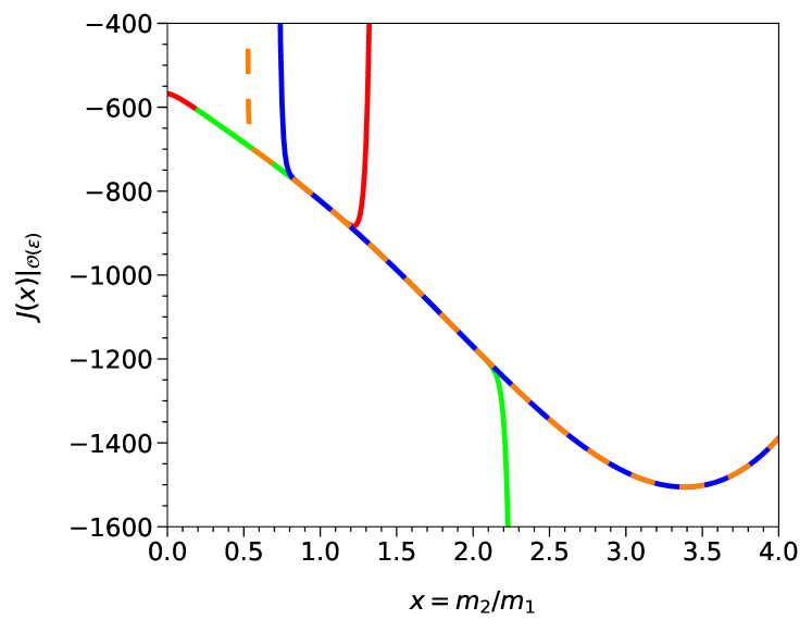
Figure 3: ${\cal O}(\epsilon)$ term of the integral $J$. The solid red, green and blue curves correspond to the expansions in $x$, $1-x$ and $1/x$. For the dashed orange curve the expansion parameter $1-1/x$ has been used.

In Fig. 3 we show results for the ${\cal O}(\epsilon)$ term of $J(x)$ for $0\leq x\leq 4$ where the red, green and blue solid curves correspond to the expansions in $x$, $1-x$ and $1/x$, including 50 expansion terms. They are the immediate results of our method and perfectly cover the whole $x$ range. The dashed orange curve corresponds to the expansion in $1-1/x$ which is obtained from the $1-x$ expansion. It is interesting to note that the green curve leads to better results for $x<1$ whereas $(1-1/x)$ is the better choice for the expansion parameter for $x>1$. In fact, in the plot there is no visible difference between the blue and orange curve. Even for x=8 the deviation is still below 10%.

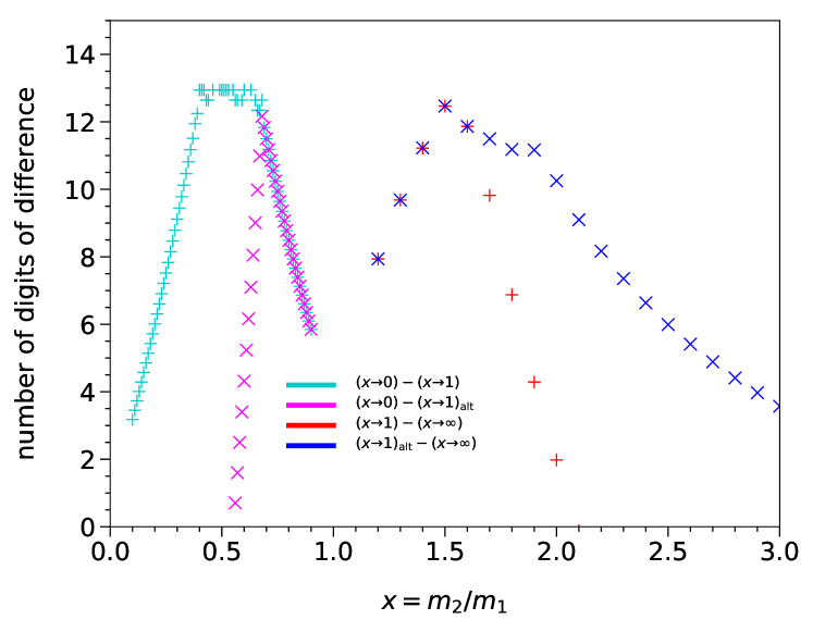
Figure 4: Difference of expansions. The number of digits on the $y$ axis is given by “$-\log_{10}(\mbox{difference})$”.

Let us next discuss the numerical accuracy. We remark that we can reproduce the analytic result for $x=0$ in Eq. (3) with a relative precision of $10^{-13}$ for the ${\cal O}(\epsilon)$ term. The lower $\epsilon$ terms are even more precise; for example, the ${\cal O}(\epsilon^{0})$ term has a precision of $10^{-17}$. Remember that $J(0)$ is obtained from analytic calculations at $x\to\infty$ and numerical matching for $x=0.5$ and $x=1.5$. In order to quantify the quality of the approximations we consider in Fig. 4 differences of expansions of the ${\cal O}(\epsilon)$ term. The interesting regions are around the matching points $x=0.5$ and $x=1.5$ where we observe differences of order $10^{-12}$ to $10^{-13}$. Taking into account that the ${\cal O}(\epsilon)$ term itself is of order $10^{2}-10^{3}$ (cf. Fig. 3) we can claim a relative precision of more than 14 digits. Away from the matching points the respective expansion provides even better results.

In Fig. 4 we show two versions of the expansion around $x=1$. The cyan and red curves use $(1-x)$ as expansion parameter and the pink and blue curves use $(1-1/x)$. As already observed in Fig. 3 we again deduce that $(1-1/x)$ is a better choice for $x>1$ whereas $(1-x)$ is better suited from $x<1$.

In Ref. [7] expansions for all 339 master integrals have been obtained and then the mass relations for the eight colour factors of Eq. (1) have been constructed. In Ref. [7] also (exact) analytic results for all 339 master integrals have been computed. This allows for a comparison of the final physical quantity. We could show that the agreement between the exact and approximated results is at least 10 significant digits for the bare four-loop quantity. For most colour factors this is also true for the renormalized quantities. Due to logarithmic divergences (e.g., the colour structure $C_{F}^{2}n_{l}n_{h}$ for $x\to 0$) one observes strong cancellations in some regions of the parameters space. However, we still have 5 significant digits in the final expression. For more details we refer to Ref. [7]. This is promising for the remaining eight colour factors where most likely no analytic results in terms of iterated integrals can be obtained.

4 Conclusion

In this contribution we have described a method which can be used to obtain semi-analytic results for multi-loop problems which depend on one parameter $x$. As an example four-loop corrections to the heavy quark mass relation with two mass scales, $m_{1}$ and $m_{2}$, have been considered. Using analytic results for $m_{2}\gg m_{1}$ it is possible to use the differential equations for the master integrals to transfer the information to $x=0$. The comparison to the known analytic result shows that a precision between 5 and 10 digits can be obtained. Using deeper expansions and/or further intermediate matching points even a higher accuracy can be achieved. Detailed result for one of the master integrals has been presented in this contribution. For the results of the mass relation we refer to Ref. [7].

References

- [1] R. Boughezal, M. Czakon and T. Schutzmeier, “NNLO fermionic corrections to the charm quark mass dependent matrix elements in ,” JHEP 09 (2007), 072, 10.1088/1126-6708/2007/09/072, [arXiv:0707.3090 [hep-ph]].
- [2] R. N. Lee, A. V. Smirnov and V. A. Smirnov, “Solving differential equations for Feynman integrals by expansions near singular points,” JHEP 03 (2018), 008, 10.1007/JHEP03(2018)008, [arXiv:1709.07525 [hep-ph]].
- [3] X. Liu, Y.-Q. Ma and C.-Y. Wang, “A Systematic and Efficient Method to Compute Multi-loop Master Integrals,” Phys. Lett. B 779 (2018), 353-357, 10.1016/j.physletb.2018.02.026, [arXiv:1711.09572 [hep-ph]].
- [4] J. Blümlein and C. Schneider, “The Method of Arbitrarily Large Moments to Calculate Single Scale Processes in Quantum Field Theory,” Phys. Lett. B 771 (2017), 31-36, 10.1016/j.physletb.2017.05.001, [arXiv:1701.04614 [hep-ph]].
- [5] F. Moriello, “Generalised power series expansions for the elliptic planar families of Higgs + jet production at two loops,” JHEP 01 (2020), 150, 10.1007/JHEP01(2020)150, [arXiv:1907.13234 [hep-ph]].
- [6] M. Hidding, “DiffExp, a Mathematica package for computing Feynman integrals in terms of one-dimensional series expansions,” Comput. Phys. Commun. 269 (2021), 108125, 10.1016/j.cpc.2021.108125, [arXiv:2006.05510 [hep-ph]].
- [7] M. Fael, F. Lange, K. Schönwald and M. Steinhauser, “A semi-analytic method to compute Feynman integrals applied to four-loop corrections to the -pole quark mass relation,” JHEP 09 (2021), 152, https://doi.org/10.1007/JHEP09(2021)152 [arXiv:2106.05296 [hep-ph]].
- [8] P. Marquard, A. V. Smirnov, V. A. Smirnov and M. Steinhauser, “Quark Mass Relations to Four-Loop Order in Perturbative QCD,” Phys. Rev. Lett. 114 (2015), 142002, 10.1103/PhysRevLett.114.142002, [arXiv:1502.01030 [hep-ph]].
- [9] P. Marquard, A. V. Smirnov, V. A. Smirnov, M. Steinhauser and D. Wellmann, “-on-shell quark mass relation up to four loops in QCD and a general SU gauge group,” Phys. Rev. D 94 (2016), 074025, 10.1103/PhysRevD.94.074025, [arXiv:1606.06754 [hep-ph]].
- [10] S. Bekavac, A. Grozin, D. Seidel and M. Steinhauser, “Light quark mass effects in the on-shell renormalization constants,” JHEP 10 (2007), 006, 10.1088/1126-6708/2007/10/006, [arXiv:0708.1729 [hep-ph]].
- [11] M. Fael, K. Schönwald and M. Steinhauser, “Exact results for and with two mass scales and up to three loops,” JHEP 10 (2020), 087, 10.1007/JHEP10(2020)087, [arXiv:2008.01102 [hep-ph]].