3D template-based -LAT constraints on the diffuse supernova
axion-like particle background¹

Abstract

Axion-like particles (ALPs) may be abundantly produced in core-collapse (CC) supernovae (SNe), hence the cumulative signal from all past SN events can create a diffuse flux peaked at energies of about 25 MeV. We improve upon the modeling of the ALPs flux by including a set of CC SN models with different progenitor masses, as well as the effects of failed CC SNe – which yield the formation of black holes instead of explosions. Relying on the coupling strength of ALPs to photons and the related Primakoff process, the diffuse SN ALP flux is converted into gamma rays while traversing the magnetic field of the Milky Way. The spatial morphology of this signal is expected to follow the shape of the Galactic magnetic field lines. We make use of this via a template-based analysis that utilizes 12 years of -LAT data in the energy range from 50 MeV to 500 GeV. In our benchmark case of the realization of astrophysical and cosmological parameters, we find an upper limit of $g_{a\gamma}\lesssim 3.76\times 10^{-11}\;\mathrm{GeV}^{-1}$ at 95$\%$ confidence level for $m_{a}\ll 10^{-11}$ eV, while we find that systematic deviations from this benchmark scenario induce an uncertainty as large as about a factor of two. Our result slightly improves the CAST bound, while still being a factor of six (baseline scenario) weaker than the SN1987A gamma-ray burst limit.

I Introduction

Observing a supernova (SN) provides unique opportunities for fundamental physics. In particular, they are ideally suited to probe feebly interacting particles (cf. Agrawal et al. (2021) for a recent review) with masses up to the $\sim 100\,{\rm MeV}$ range. Indeed, large numbers of such particles can be emitted in SN events Raffelt (1996). An important and theoretically interesting instance of this are axions and axion-like particles (ALPs) Raffelt (2008); Fischer et al. (2016). Indeed, SN 1987A has significantly strengthened astrophysical axion bounds in a region of the yet-incompletely known ALP parameter space, complementary to the one probed by the Sun and the globular clusters Raffelt (2008); Brockway et al. (1996); Grifols et al. (1996); Carenza et al. (2019); Lucente et al. (2020). In the minimal scenario in which ALPs are coupled only with photons, the main channel for their emissivity in the SN core is the Primakoff process, leading to an ALP flux peaked at energies of about 25 MeV. Conversion of these ALPs into gamma rays in the Milky Way magnetic field can lead to an observable gamma-ray burst in coincidence with the SN explosion Brockway et al. (1996); Grifols et al. (1996). At the time of the SN 1987A, the Gamma-Ray Spectrometer (GRS) on the Solar Maximum Mission (SMM) observed no gamma-ray signal at the time of the SN explosion, this made possible to constrain the photon-ALP coupling early on (see Brockway et al. (1996); Grifols et al. (1996) for a detailed discussion). In a more refined, recent analysis, this upper limit is stated as $g_{a\gamma}\lesssim 5.3\times 10^{-12}\,\textrm{GeV}^{-1}$ for $m_{a}<4\times 10^{-10}$ eV Payez et al. (2015). X-ray observations of super star clusters in the vicinity of the Milky Way’s Galactic center can further strengthen this bound to $g_{a\gamma}\lesssim 3.6\times 10^{-12}\,\textrm{GeV}^{-1}$ for $m_{a}<5\times 10^{-11}$ eV at $95\%$ confidence level (CL) Dessert et al. (2020). A future Galactic SN explosion in the field of view of the Large Area Telescope (LAT) aboard the  satellite would allow us to constrain $g_{a\gamma}\lesssim 2.0\times 10^{-13}\,\textrm{GeV}^{-1}$ for $m_{a}<10^{-9}$ eV Meyer et al. (2017). Furthermore, a search for gamma-ray bursts from extragalactic SNe with -LAT has yielded the limit $g_{a\gamma}\lesssim 2.6\times 10^{-11}\,\textrm{GeV}^{-1}$ for $m_{a}<3\times 10^{-10}$ eV Meyer and Petrushevska (2020) (see also Meyer and Petrushevska (2021); Crnogorčević et al. (2021)).

While a single SN event is rare (Diehl et al., 2006) and must fall into the detector field of view to be observed, there exists a guaranteed contribution to the gamma-ray diffuse flux which originates from ALPs emitted by all past SNe in the Universe Raffelt et al. (2011). This Diffuse SN ALP Background (DSNALPB), despite being fainter than the Galactic one, is within the reach of the -LAT experiment. In Ref. Calore et al. (2020), henceforth called ‘Paper I’, some of us used published -LAT observations of the gamma-ray isotropic diffuse background to set a bound $g_{a\gamma}\lesssim 5.0\times 10^{-11}\,\textrm{GeV}^{-1}$ for $m_{a}<10^{-11}$ eV. However, this analysis does not completely acknowledge some technical issues behind the derivation of the isotropic gamma-ray background, which may impact the reliability of the stated upper bound on $g_{a\gamma}$. This component of the gamma-ray sky is obtained in connection with a particular model of the diffuse gamma-ray flux from the Milky Way and evaluated in a particular region of interest (ROI). Both the dependence on the diffuse model and the dependence on the selected sky region introduce unknowns in the upper bound estimate that cannot be cast into an uncertainty on the derived value because it is not known if the initial choices made by the -LAT collaboration create artificially strong or weak limits. Hence, we deem it warranted to put the analysis of the DSNALPB on solid statistical foundations by creating a complete -LAT data analysis pipeline which takes into account all the experience that has been gained over the long run of the LAT.

In the present work, we improve upon the previous analysis presented in Paper I in two ways. First, we present a more refined model of the SNe ALPs flux. It is indeed well known that the production of ALPs in a SN event depends on the progenitor mass. In Paper I, however, it was assumed that all past SNe are represented by a 18 $M_{\odot}$ progenitor model. Here, instead, we consider different CC SN models with masses ranging between 8.8 and 70 $M_{\odot}$, accounting also for the contribution due to failed core-collapse (CC) SN explosions. This allows us to determine with better accuracy a possible range of variability of the DSNALPB, and, in turn, of the expected gamma-ray flux. Secondly, we try to exploit the full potential of -LAT data in searching for this type of signal, by including information on the expected spatial structure of the signal in the gamma-ray data analysis. Paper I indeed sets limits on ALPs solely making use of the spectral energy distribution of the data. On the other hand, template-based analyses – see e.g. Mattox et al. (1996) for an early application in the context of EGRET data or a more recent example of an analysis of Fermi-LAT data Su et al. (2010) that led to the discovery of the so-called Fermi Bubbles – exploit both spectral and spatial properties of gamma-ray data to constrain physics models. This gamma-ray fitting technique has proven to be particularly successful in testing the hypothesis of weakly interacting massive particles shining in gamma rays at GeV - TeV energies (see, for instance, Ackermann et al. (2012, 2017); Storm et al. (2017); Di Mauro et al. (2019); Di (2021)). However, to our knowledge, it was never applied to the search of an ALPs signal, albeit it presents specific spatial features, as we discuss below. We therefore perform a template-based analysis to constrain the ALP parameter space via the spatial structure of the DSNALPB induced diffuse gamma-ray flux using 12 years of -LAT data in the energy range from 50 MeV to 500 GeV.

The paper is organized as follows. In Sec. II, we illustrate the CC SN models based on state-of-the-art hydrodynamical simulations. In Sec. III, we present our updated calculation of the ALPs production flux in SNe and induced gamma-ray flux from the DSNALPB. In Sec. IV, we sketch the analysis framework: data selection and preparation, and template fitting method of -LAT data. We discuss our results in Sec. V. We discuss systematic uncertainties and their impact on the ALPs upper limits in Sec. VI, and conclude in Sec. VII. Two final appendices are devoted to more technical issues. In Appendix

A we characterize some details concerning the calculation of the SN ALP spectrum, namely the effect of the presence of alpha particles in the SN core and the effects of the gravitational energy-redshift due to the strong gravitational field of the proto-neutron star, which were overlooked in previous analyses. In Appendix B, we present more details on the systematic uncertainty on the DSNALPB upper limits of cosmological and astrophysical origin.

II Core-collapse supernova models

In order to provide reliable constraints on the DSNALPB, it is essential to cover a representative, wide range of SN models, which are based on state-of-the-art simulations. The present work discusses SN simulations which are based on general relativistic neutrino radiation hydrodynamics featuring three-flavor neutrino transport, both in spherical symmetry Mezzacappa and Bruenn (1993); Liebendörfer et al. (2004); Fischer (2016); Fischer et al. (2020) with accurate Boltzmann neutrino transport, and in axial symmetry with a multi-energy neutrino transport method Kuroda et al. (2021). These simulations implement a complete set of weak interactions Kotake et al. (2018), and a multi-purpose microscopic nuclear matter equation of state (EOS) Lattimer and Swesty (1991); Shen et al. (1998); Hempel and Schaffner-Bielich (2010); Hempel et al. (2012); Steiner et al. (2013).

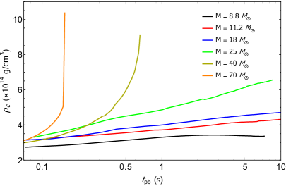
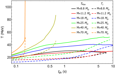
Figure 1: PNS evolution during the deleptonization phase for the SN explosion models launched from different progenitors with ZAMS masses of 8.8, 11.2, 18.0 and $25~{}M_{\odot}$. Left panel: central density, $\rho_{\rm centre}$. Right panel: central and maximum temperatures, $T_{\rm centre}$ (dashed lines) and $T_{\rm Max}$ (solid lines). fig:rho˙T

In what follows, we distinguish successful core-collapse SN explosions of different types of progenitors. We consider the low-mass oxygen-neon-magnesium core progenitor with zero-age main sequence (ZAMS) mass of $8.8~{}M_{\odot}$ Nomoto (1987). They belong to the class of electron-capture SN Kitaura et al. (2006), which yield neutrino-driven SN explosions even in spherical symmetry. The SN simulations discussed here were reported in Ref. Fischer et al. (2010), based on the nuclear EOS of Ref. Shen et al. (1998). The simulations include all SN phases, i.e. stellar core collapse, core bounce with the formation of the bounce shock, the subsequent SN post-bounce mass accretion phase including the explosion onset with the revival of the stalled bounce shock and finally the long-term deleptonization phase of the compact hot and dense central remnant proto-neutron star (PNS). The latter SN phase is of particular importance for the emission of axions. The remnant of this electron-capture SN explosion is a low-mass neutron star with a baryon mass of about $1.37~{}M_{\odot}$. The corresponding PNS deleptonization features a nearly constant central density of $\rho_{\rm central}\simeq 3.5\times 10^{14}$ g cm^-3 as well as central temperature decreasing from $T_{\rm Max}\simeq 30$ MeV to 25 MeV during the PNS deleptonization up to about 7.5 s post bounce, as illustrated in Fig. LABEL:fig:rho_T. In addition to the decreasing, central temperature, we show the maximum temperature evolution in Fig. LABEL:fig:rho_T, which rises moderately from $T_{\rm core}\simeq 20$ MeV to about 25 MeV.

As an example of a low-mass iron-core progenitor we consider the example with ZAMS mass of $11.2~{}M_{\odot}$ from the stellar evolution series of Ref. Woosley et al. (2002). In contrast to electron-capture SN, which are characterized by a short post-bounce mass accretion period on the order of only few tenths of a second before the onset of the explosion, more massive iron-core progenitors suffer from extended post-bounce mass accretion periods, which fail to yield neutrino-driven explosions in self-consistent spherically symmetric simulations. Nevertheless, in order to obtain explosions, the neutrino heating and cooling rates have been enhanced artificially in Ref. Fischer et al. (2010), which lead to the successful revival of the stalled bounce shock. It results in the SN explosion onset about 300 ms after core bounce, for this progenitor star of $11.2~{}M_{\odot}$. The subsequent evolution of the central density of $\rho_{\rm centre}\simeq 4\times 10^{14}$ g cm^-3 as well as the central and maximum temperatures is illustrated in Fig. LABEL:fig:rho_T. The latter differ only marginally from those of the $8.8~{}M_{\odot}$ model.

Two more massive iron-core progenitors are included here, with ZAMS masses of $18.0~{}M_{\odot}$ and $25~{}M_{\odot}$, which are evolved in a similar fashion as the $11.2~{}M_{\odot}$ model leading to neutrino-driven SN explosions on the order of several hundreds of milliseconds after core bounce. However, the remnant PNSs are more massive and hence feature a higher central density as well as higher central and maximum temperatures than the 8.8 and $11.2~{}M_{\odot}$ models (see Fig. LABEL:fig:rho_T). In particular the $25~{}M_{\odot}$ simulation reaches maximum temperatures at the PNS interior which reach as high as 50 MeV during the PNS deleptonization phase. This aspect is important for the axion emission since the axion emissivity has a strong temperature dependence.

In addition to the successful CC SN explosion models, we consider two examples with ZAMS masses of $40$ and $70~{}M_{\odot}$ belonging to the failed CC SN branch which yield the formation of black holes instead Baumgarte et al. (1996); Sumiyoshi et al. (2006); Fischer et al. (2009); O’Connor and Ott (2011). In such case the mass accretion onto the bounce shock, in combination with the failed shock revival, leads to the continuous growth of the enclosed mass of the PNS until it exceeds the maximum mass given by the nuclear EOS, on a timescale of several hundreds of milliseconds up to one second post bounce. If no phase transition is considered Fischer et al. (2018); Fischer (2021), the PNS collapses eventually and a black hole forms. The data for the SN simulation of the $40~{}M_{\odot}$ progenitor discussed in the following are taken from Ref. Fischer et al. (2009) based on the nuclear EOS of Ref. Lattimer and Swesty (1991). It results in black hole formation at about 450 ms post bounce with an enclosed PNS mass of about $2.5~{}M_{\odot}$. The most massive progenitor model considered of $70~{}M_{\odot}$, belongs to the class of zero-metallicity stars (Takahashi et al., 2014) for which a black hole forms within a few hundred milliseconds after core bounce (Kuroda et al., 2018; Shibagaki et al., 2021; Kuroda et al., 2021). This model has been evolved in axially symmetric simulations. Although the original SN simulation (Kuroda et al., 2021) takes into account the effect of strong phase transition from nuclear matter to the quark-gluon plasma at high baryon density, the central quark core immediately collapses into a BH within $\sim 1$ ms after its formation. Therefore its influence on ALP emission is expected to be minor. Furthermore, as the central high temperature region is swallowed by the BH, most of the ALP emission is expected to cease abruptly once the BH formation occurs, as indicated by ending the lines in Fig. LABEL:fig:rho_T. The corresponding baryonic PNS mass at the onset of the PNS collapse is estimated to be $\sim 2.6~{}M_{\odot}$. In comparison to the other SN explosion models, with ZAMS masses of $8.8-25~{}M_{\odot}$, the failed SN branch yields significantly higher central densities as well as core temperatures. The latter reaches shortly before black hole formation up to $\rho_{\rm centre}\geq 10^{15}$ g cm^-3 and $T_{\rm Max}\geq 100$ MeV.

Having a set of characteristic supernovae, we will then do a simple interpolation between them, as will be described below.

III DSNALPB and gamma-ray flux

III.1 ALPs emission from SNe

We consider a minimal scenario in which ALPs have only a two-photon coupling, characterized by the Lagrangian Raffelt and Stodolsky (1988)

$${\cal L}_{a\gamma}=-\frac{1}{4}\,g_{a\gamma}F_{\mu\nu}\tilde{F}^{\mu\nu}a=g_{a\gamma}\,{\bf E}\cdot{\bf B}\,a~{}.$$ (1)

Through this interactions ALPs may be produced in stellar plasma primarily via the Primakoff process Raffelt (1986). In such a process thermal photons are converted into ALPs in the electrostatic field of ions, electrons and protons. We calculate the ALP production rate (per volume) in a SN core via Primakoff process closely following Payez et al. (2015), which finds

$$\dfrac{d\dot{n}_{a}}{dE} = \frac{g_{a\gamma}^{2}\xi^{2}\,T^{3}\,E^{2}}{8\pi^{3}\,\left(e^{E/T}-1\right)}$$ (2)

$$\left[\left(1+\dfrac{\xi^{2}T^{2}}{E^{2}}\right)\ln(1+E^{2}/\xi^{2}T^{2})-1\right]\,.$$

Here, $E$ is the photon energy measured by a local observer at the emission radius, $T$ the temperature and $\xi^{2}={\kappa^{2}}/{4T^{2}}$ with $\kappa$ the inverse Debye screening length, describing the finite range of the electric field surrounding charged particles in the plasma. The total ALP production rate per unit energy is obtained integrating Eq. (2) over the SN volume. Details on the calculation of the SN ALP spectrum are provided in Appendix A. In particular, we discuss the enhancement of the ALP flux associated with the presence of alpha particles in the SN core. Furthermore we also show that the strong gravitational field of a proto-neutron star can modify the ALP emissivity in the SN core via three General Relativistic effects: time dilation, trajectory bending and energy redshift. As explained in Appendix A.2, the trajectory bending has no effect on the time-integrated diffuse ALP background we aim to calculate. Therefore, we will focus only on energy-redshift and time-dilation here.

Assuming $m_{a}\ll T$, the ALP fluence is given, with excellent precision, by the analytical expression Payez et al. (2015)

$$\frac{dN_{a}}{dE}=C\left(\frac{g_{a\gamma}}{10^{-11}\textrm{GeV}^{-1}}\right)^{2}\left(\frac{E}{E_{0}}\right)^{\beta}\exp\left(-\frac{(\beta+1)E}{E_{0}}\right)\,,$$ (3)

where the values of the parameters $C$, $E_{0}$, and $\beta$ for the SN models with different progenitors are given in Table 1. The spectrum described in Eq. (3) is a typical quasi-thermal spectrum, with mean energy $E_{0}$ and index $\beta$ (in particular, $\beta=2$ corresponds to a perfectly thermal spectrum of ultrarelativistic particles).

Table 1: Fitting parameters for the SN ALP spectrum, Eq. (3), from the Primakoff process for different SN progenitors.

SN progenitor	$C$ [$\times 10^{50}\,\ {\rm MeV}^{-1}$]	$E_{0}$ [MeV]	$\beta$
8.8 $M_{\odot}$	$3.76\,\$	76.44	2.59
11.2 $M_{\odot}$	$7.09\,\$	75.70	2.80
18 $M_{\odot}$	$23.0\,\$	91.61	2.43
25 $M_{\odot}$	$28.1\,\$	105.5	2.30
40 $M_{\odot}$	$2.48\,\$	112.7	1.92
70 $M_{\odot}$	$0.391\,\$	30.44	0.785

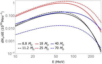
Figure 2: Produced SN ALP number as a function of energy for different SN progenitor mass. We assume $g_{a\gamma}=10^{-11}\operatorname{GeV}^{-1}$.

In Fig. 2, we represent the SN ALP spectra from different progenitors. We realize that for the successful CC SN explosions the average energy $E_{0}$ increases monotonically with the progenitor mass, as well as the peak of the spectrum. For the failed CC SN explosions, since the emitted flux is integrated over a shorter time window, the flux is suppressed with respect to the previous models.

For further purposes related to the calculation of the DSNALPB it is useful to determine the variation of the spectral coefficients $C$, $E_{0}$, and $\beta$ as a function of the SN progenitor mass. Given the sparseness of the data we assume a linear behaviour in the range $[8;30]M_{\odot}$, as shown in Fig. 3. The functional expressions are the following ones

$$\frac{C(M)}{10^{50}\,\ \textrm{MeV}^{-1}} = (1.73\pm 0.172)\frac{M}{M_{\odot}}-9.74\pm 2.92\,\ ,$$

$$\frac{E_{0}(M)}{\textrm{MeV}} = (1.77\pm 0.156)\frac{M}{M_{\odot}}+59.3\pm 2.65\,\ ,$$

$$\beta(M) = (-0.0254\pm 0.00587)\frac{M}{M_{\odot}}+2.94\pm 0.0997\,\ ,$$

where the quoted errors represent the standard mean-square uncertainties associated with the linear regression, and are taken into account into the final evaluation of the uncertainty on the bound.

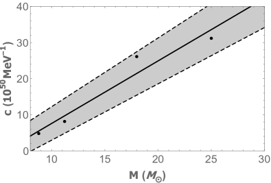
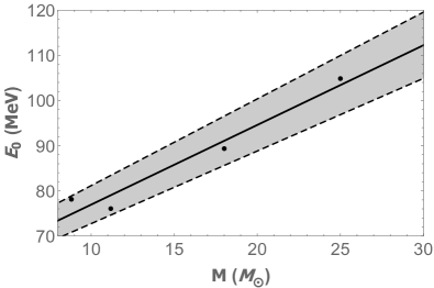
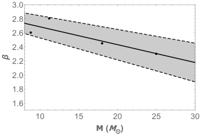
Figure 3: Variation of spectral parameters of Eq. (3) as a function of the SN progenitor mass. We assume $m_{a}\ll 10^{-11}$ eV and $g_{a\gamma}=10^{-11}\operatorname{GeV}^{-1}$.

For failed CC SN explosions, we only have two models from different groups, and therefore we do not attempt any interpolation.

III.2 Diffuse SN ALP background

From the SN ALP flux described in the previous section, one can calculate the DSNALPB from all past CC SNe in the Universe, as in Paper I (see also Beacom (2010); Raffelt et al. (2011) and in particular Sec. VI of Ref. Caputo et al. (2021) for a detailed derivation of this equation),

$$\frac{d\phi_{a}(E_{a})}{dE_{a}}\!\! = \!\!\int_{0}^{\infty}\!\left[(1+z)\frac{dN_{a}^{CC}(E_{a}(1+z))}{dE_{a}}\right]$$

$$\times [R_{CC}(z)]\bigg{[}\bigg{|}c\frac{dt}{dz}\bigg{|}dz\bigg{]}.$$

The first term in large brackets is the emission spectrum $dN_{a}^{CC}/dE_{a}$, where an ALP received at energy $E_{a}$ was emitted at a higher energy $E_{a}(1+z)$; the prefactor of $(1+z)$ on the spectrum accounts for the compression of the energy scale, due to the redshift $z$. The second term is the supernova rate density $R_{CC}(z)$. The third term is the differential distance where $|{dt}/{dz}|^{-1}=H_{0}(1+z)[\Omega_{\Lambda}+\Omega_{M}(1+z)^{3}]^{1/2}$ with the cosmological parameters $H_{0}=67$ km s^-1 Mpc^-1, $\Omega_{M}=0.3$, $\Omega_{\Lambda}=0.7$.

ALP spectrum from past core-collapse SNe. In order to calculate the ALP spectrum of past CC SN events $dN_{a}^{CC}/dE_{a}$, one has to weight the flux from a given CC SN over the initial mass function (IMF) which provides the number of stars formed per unit of mass as function of the progenitor mass $M$.

Following Ref. Horiuchi et al. (2009), we show the results for three IMFs: a traditional Salpeter IMF Salpeter (1955), an intermediate Kroupa IMF Kroupa (2001), and a shallower Baldry-Glazebrook (BG) IMF Baldry and Glazebrook (2003). The different IMF are characterized by the parameter $\zeta$, defined in the expression below

$$\phi(M)\propto M^{-\zeta}\,\ .$$ (6)

For $M\gtrsim 0.5M_{\odot}$, we find $\zeta=2.35$ for the Salpeter IMF, $\zeta=2.3$ for the Kroupa case and $\zeta=2.15$ for the BG IMF.

It is expected that the IMF of stars may depend systematically on the environment. In this context, in Ref. Gutcke and Springel (2019) it was suggested to empirically investigate the effect of metallicity changing the exponent $\zeta$ in a range $[0.34:3.44]$. We find that the effect can produce a factor $\sim 2$ change in the DNSALPB flux.

In our study, we consider masses from 8 up to 125 $M_{\odot}$. However, due to the steep decline of Eq. (6), the high-mass end is suppressed and thus of minor relevance for the DSNALPB. The IMF-weighted ALP spectrum $dN_{a}^{CC}/dE_{a}$ of all CC SN events can then be calculated as Kresse et al. (2021)

$$\frac{dN_{a}^{CC}}{dE_{a}}=\frac{\int_{\Lambda_{\rm expl-CC}}dM\phi(M)\frac{dN_{a}}{dE}(M)+\int_{\Lambda_{\rm fail-CC}}dM\phi(M)\frac{dN_{a}}{dE}(M)}{\int_{8M_{\odot}}^{125M_{\odot}}dM\phi(M)}\,\ ,$$ (7)

where $\Lambda_{\rm expl-CC}$ and $\Lambda_{\rm fail-CC}$ represent the domains in the progenitor mass range where one expects to have a successful and a failed CC SN explosion progenitor, respectively. In particular, the domain of failed CC SN explosions is defined following Møller et al. (2018):

$$f_{\rm fail-CC}=\frac{\int_{\Lambda_{\rm fail-CC}}dM\phi(M)}{\int_{8M_{\odot}}^{125M_{\odot}}dM\phi(M)}\,\ ,$$ (8)

and implemented here as an hard cut $M^{\rm min}_{\rm fail-CC}$, which represents the lower mass bound of the failed CC SN explosions domain. From here, it also follows that $f_{\rm expl-CC}=1-f_{\rm fail-CC}$.

In order to study the DSNALPB sensitivity to $f_{\rm fail-CC}$ we consider four different scenarios, as in  Møller et al. (2018). Each scenario is characterized by a different $M^{\rm min}_{\rm fail-CC}$. We consider that all stars with $M>M^{\rm min}_{\rm fail-CC}$ evolve into BH-SNe. For progenitor masses lower than $M^{\rm min}_{\rm fail-CC}$ we assume successful explosions with spectrum in Eq. (3) following the scaling of the parameters given by Eq. (LABEL:eq:parameters). Instead, we model failed CC SNe explosions as the 40 $M_{\odot}$ model for $M^{\rm min}_{\rm fail-CC}<M<$ 60 $M_{\odot}$. In the range $[60:125]M_{\odot}$ they are represented by the $70M_{\odot}$ model. The four scenarios are:

• $f_{\rm fail-CC}=10\%$: $M^{\rm min}_{\rm fail-CC}=36M_{\odot}$, see e.g. Woosley et al. (2002); Pejcha and Thompson (2015). This is a (as concerns ALPs) optimistic scenario where the fraction of SNe leading to black hole formation is small.

• $f_{\rm fail-CC}=20\%$: $M^{\rm min}_{\rm fail-CC}=24.0$ $M_{\odot}$, following Refs. Ertl et al. (2016); Raithel et al. (2018).

• $f_{\rm fail-CC}=30\%$: $M^{\rm min}_{\rm fail-CC}=18.5$ $M_{\odot}$.

• $f_{\rm fail-CC}=40\%$: $M^{\rm min}_{\rm fail-CC}=15.0$ $M_{\odot}$. This is based on the findings of Ref. Sukhbold et al. (2016); Hidaka et al. (2016) and it is still well within the observational constraints Adams et al. (2017).

In principle, it has been recently shown that the appearance of exotic phases of hot and dense matter, associated with a sufficiently strong phase transition from nuclear matter to the quark-gluon plasma at high baryon density, can trigger supernova explosions of massive stars in the range $35-50$ $M_{\odot}$. However, from nucleosynthesis studies it results that the contribution of these exotic SNe might be at most 1 % of the total ones Fischer et al. (2020). Therefore, their contribution to the DSNALPB is negligible and we will neglect it hereafter.

Supernova rate $R_{\rm CC}$. The intensity and spectrum of the DSNALPB depend on the cosmological rate of core collapse (or, shortly, Supernova Rate, SNR). The SNR, differential in the progenitor mass $M$, is proportional to the star formation rate (SFR), $R_{\rm SF}(z)$ (defined as the mass that forms stars per unit comoving volume per unit time, at redshift $z$) Lunardini (2016); Møller et al. (2018):

$$R_{\rm CC}(z,M)=R_{\rm SF}(z)\frac{\int_{8.0M_{\odot}}^{125M_{\odot}}dM\phi(M)}{\int_{0.5M_{\odot}}^{125M_{\odot}}dMM\phi(M)}\,\ .$$ (9)

The SFR is well described by the functional fit Yuksel et al. (2008)

$$R_{\rm SF}(z)=R_{\rm SF}(0)\biggl{[}(1+z)^{\alpha\eta}+\biggl{(}\frac{1+z}{B}\biggr{)}^{\beta\eta}+\biggl{(}\frac{1+z}{D}\biggr{)}^{\gamma\eta}\biggr{]}^{1/\eta}\;.$$ (10)

where $R_{\rm SF}(0)$ is the normalization (in units of $M_{\odot}\,\ \textrm{yr}^{-1}\,\ \textrm{Mpc}^{-3}$) , $B$ and $D$ encode the redshift breaks, the transitions are smoothed by the choice $\eta\simeq-10$, and $\alpha$, $\beta$ and $\gamma$ are the logarithmic slopes of the low, intermediate, and high redshift regimes, respectively. The constants $B$ and $D$ are defined as

$$B = (1+z_{1})^{1-\alpha/\beta}\,\ ,$$

$$D = (1+z_{1})^{(\beta-\alpha)/\gamma}(1+z_{2})^{1-\beta/\gamma}\,\ ,$$ (11)

where $z_{1}$ and $z_{2}$ are the redshift breaks. All the parameters of the model are collected in Tab. 2 based on Horiuchi et al. (2009). In the Table the parameters refer to the Salpeter IMF. For the Kroupa and the BG IMFs the normalization factor is reduced by $\simeq 0.94$ and $\simeq 0.76$, respectively, while the overall shape is not greatly affected (see Table 2 of Hopkins and Beacom (2006)).

Table 2: Model parameters for the SFR, Eq. (10), values taken from Horiuchi et al. (2009).

Analytic fits	$R_{\rm SF}(0)$	$\alpha$	$\beta$	$\gamma$	$z_{1}$	$z_{2}$
Upper	0.0213	3.6	-0.1	-2.5	1	4
Fiducial	0.0178	3.4	-0.3	-3.5	1	4
Lower	0.0142	3.2	-0.5	-4.5	1	4

DSNALPB flux. We are now ready to discuss how the different uncertainties in the calculation discussed above impact the DSNALPB flux. In Fig. 4 we show the DSNALPB fluxes for a photon coupling $g_{a\gamma}=10^{-11}$ GeV^-1 and $m_{a}\ll 10^{-11}$ eV for the different fractions of failed SNe $f_{\rm fail-CC}$, assuming the fiducial model of Table 2 for the $R_{\rm SF}$. As expected, the larger $f_{\rm fail-CC}$ the more suppressed is the flux. The flux uncertainty related to the unknown fraction of failed SNe is a factor $\sim 3$.

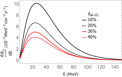
Figure 4: DSNALPB fluxes with $g_{a\gamma}=10^{-11}$ GeV^-1 for different fractions of failed SNe $f_{\rm fail-CC}$, assuming the fiducial model for $R_{\rm SF}$.

In Fig. 5 we show the impact of the changes of parameters in the $R_{\rm SF}$ of Table 3. We fix $f_{\rm fail-CC}=10\%$ and Salpeter IMF. The continuous curve refers to the fiducial model for $R_{\rm SF}$, while upper and lower curves refer to upper and lower models, respectively. The uncertainty on $R_{\rm SF}$ leads to a factor $\sim 3$ of variation in the DSNALPB flux. Instead, the variation associated with a different choice of IMF is subleading.

Finally, we include all the different uncertainties related to the fraction of failed SNe, to the SNR and IMF in order to get a range of variability for the DSNALPB, as shown in the gray band in Fig. 6, where the lower dashed line corresponds to $f_{\rm fail-CC}=40\%$, BG IMF and lower model parameters for $R_{\rm SF}$ in Table 3, while the upper dashed curve corresponds to $f_{\rm fail-CC}=10\%$, Salpeter IMF and upper model parameters for $R_{\rm SF}$. For comparison with the continuous curve we show the case of $f_{\rm fail-CC}=20\%$, Salpeter IMF and fiducial model parameters for $R_{\rm SF}$. We point out that the total range of variability in the DSNALPB flux is a factor $\sim 8$.

We find that the DSNALPB spectrum can also be represented by the functional form of Eq. (3). In Table 3 we show the fitting parameters for the four cases with different $f_{\rm fail-CC}$, taking a Salpeter IMF and and a fiducial model for the $R_{\rm SF}$ parameters in Table 3. Typically, in this case the average energy of the spectrum is $E_{0}\sim 40$ MeV while its maximum is attained around 25 MeV.

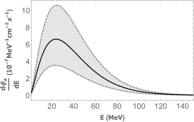
Figure 5: DSNALPB fluxes for $g_{a\gamma}=10^{-11}$ GeV^-1, $f_{\rm fail-CC}=20\%$ and the Salpeter IMF. The uncertainty range is due to the $R_{\rm SF}$ parameters of Table 3. The continuous curve refers to the fiducial model, while upper and lower curves refer to upper and lower models, respectively.

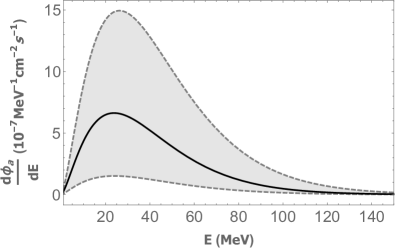
Figure 6: DSNALPB fluxes range of variability (gray band) for $g_{a\gamma}=10^{-11}$ GeV^-1. The lower dashed line corresponds to $f_{\rm fail-CC}=40\%$, BG IMF and lower model parameters for $R_{\rm SF}$ in Table 3, while the upper dashed curve corresponds to $f_{\rm fail-CC}=10\%$, Salpeter IMF and upper model parameters for $R_{\rm SF}$. The continuous curve refers to $f_{\rm fail-CC}=20\%$, Salpeter IMF and fiducial model parameters for $R_{\rm SF}$.

Table 3: Fitting parameters for DSNALPB fluxes for $g_{a\gamma}=10^{-11}$ GeV^-1 and and $m_{a}\ll 10^{-11}$ eV for different fractions of failed SNe $f_{\rm fail-CC}$, taking a Salpeter IMF and and a fiducial model for the $R_{\rm SF}$ parameters in Table 3. The case “max flux” corresponds to Salpeter IMF, and upper model parameters for $R_{\rm SF}$ in Table 3, while the case “min flux” corresponds to BG IMF and lower model parameters for $R_{\rm SF}$ in Table 3.

$f_{\textrm{fail-CC}}$	$C$ [$\times 10^{-7}\,\ {\rm MeV}^{-1}\textrm{cm}^{-2}\textrm{s}^{-1}$]	$E_{0}$ [MeV]	$\beta$
10% max flux	$144\,\$	43.8	1.50
10%	$88.9\,\$	43.5	1.41
20%	$62.9\,\$	39.9	1.49
30%	$46.5\,\$	39.3	1.47
40%	$35.8\,\$	40.2	1.41
40% min flux	$15.7\,\$	42.3	1.32

DSNALPB conversions into gamma rays. ALPs produced in a SN propagate until they reach the Milky Way, where they can convert into photons in the Galactic magnetic field (GMF). To calculate the conversion probability we follow the same procedure used in Paper I and Refs. Horns et al. (2012)).

As it is well known (see Raffelt and Stodolsky (1988) for the seminal paper discussing this in detail), in a homogeneous magnetic field, ALPs can convert into photons with a polarization parallel to the magnetic field. For massless ALPs, in vacuum and at sufficiently weak coupling the conversion probability after a length $d$ is,

$$P_{a\to\gamma} = \left(\frac{g_{a\gamma}B_{T}}{2}\right)^{2}d^{2}$$

$$\sim 0.015\left(\frac{g_{a\gamma}}{10^{-11}\,{\rm GeV}}\right)^{2}\left(\frac{B_{T}}{10^{-6}\,\rm G}\right)\left(\frac{d}{\rm kpc}\right)^{2}.$$

Here, $B_{T}$ is the magnetic field strength transverse to the propagation direction of the ALP. In the Galaxy we expect fields of the order of µG, see Jaffe (2019) for a comprehensive review. For the chosen value of the coupling we can therefore expect appreciable conversion inside the Galaxy.

However, there are additional effects that have to be taken into account to achieve a realistic description inside the Galaxy. In the Galaxy neither the strength nor the the direction of the magnetic field is constant. Therefore, one has to integrate the build up of the photon amplitude for both possible polarization directions along the line of propagation through the Galaxy. We solve the relevant equations numerically. To do so we need the Galactic magnetic field model as an input. As our baseline model we take the Jansson-Farrar model (Jansson and Farrar (2012)) with the updated parameters given in Tab. C.2 of Adam et al. (2016a) (“Jansson12c” ordered fields). To quantify the uncertainty due to the magnetic field, we also compare to the the Pshirkov model Pshirkov et al. (2011). This second model features a larger magnetic field in the Galactic plane and a weaker off-plane component, and, to the best of our knowledge, it is not excluded yet by Faraday rotation data.

The propagation is further complicated by changes in the wavelength of the photon and the ALP. These arise from the mass of the ALP, the plasma mass of the photon arising from the non-vanishing electron density, as well as, indeed, the coupling between the ALP and the photon inside the magnetic field. The ALP mass and the photon coupling are explicit parameters of the ALP model, i.e. the parameters we want to constrain. The plasma mass is directly related to the electron density which we take as an astrophysical input. For the electron density, we use the model described in Cordes and Lazio (2002) (for both magnetic field configurations). In general the effect of the photon and plasma mass on the probability is energy dependent and fully included in our analysis. We note however, that for $m_{a}\lesssim 10^{-11}\,{\rm eV}$ and $g_{a\gamma}\lesssim 10^{-11}\,{\rm GeV}$ and energies $E\gtrsim 50\,{\rm MeV}$ the mass effects become negligible and the probability is energy independent.

In Fig. 7 we show an example of the all-sky DSNALP gamma-ray flux, resulting from the numerical implementation of the procedure outlined above. For the $a\to\gamma$ conversion probability in the Milky Way, we started from a pure ALPs beam at the outside boundary of the Galaxy, for the Jansson and Farrar magnetic field model derived in Jansson and Farrar (2012) and with parameters updated according to Adam et al. (2016a). Besides giving an idea of the magnitude of fluxes at play from ALPs, this map represents the spatial distribution of the signal as it is used, for the first time in this work, as input for the -LAT analysis.

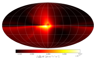
Figure 7: All-sky map in Galactic coordinates of the photon flux from the DSNALPB, $\frac{\mathrm{d}^{2}\Phi}{\mathrm{d}E\mathrm{d}\Omega}$, integrated from 50 MeV to 200 MeV (corresponding energy range of the low-energy -LAT data set used in the following analysis, see Sec. IV.1) with respect to the benchmark scenario defined in Sec. V. The assumed coupling $g_{a\gamma}=3.76\times 10^{-11}$GeV^-1 (for $m_{a}\ll 10^{-11}$ eV) represents the $95\%$ CL upper bound derived later in this analysis for the benchmark DSNALPB scenario (cf. Sec. V).

IV Fermi-LAT Analysis framework

IV.1 Data selection

We use 12 years of -LAT Pass8 data. The signal is peaked at about 25 MeV. Therefore, we use two separate data sets with different selection criteria to specifically improve the analysis of LAT data below 200 MeV. The applied criteria are summarized in Tab. 4.

Data Set	$E<200$ MeV	$E\geq 200$ MeV
Reconstruction algorithm	Pass 8
Event class	ULTRACLEANVETO
Event type	PSF3	FRONT+BACK
Energy range	50 MeV - 200 MeV	200 MeV - 500 GeV
Time interval	12 years (4th August 2008 - 3rd September 2020)
ROI	all sky
Zenith angle (applied to gtltcube)	$<90^{\circ}$
Time cuts filter	DATA_QUAL==1 && LAT_CONFIG==1
HEALPix resolution	$N_{\mathrm{side}}=64$
energy binning	30 logarithmically-spaced bins

Table 4: Data selection and preparation specifications .

While the $E<200$ MeV data is the main driver of the constraint, let us nevertheless start by describing our procedure for the more standard $E\geq 200$ MeV data set. This gives the picture of the main ingredients in our analysis. We will later comment on the adaptations for the $E<200$ MeV region.

The data set of events $E\geq 200$ MeV includes both front- and back-converted events to increase the statistical sample, whereas the data set with $E<200$ MeV is restricted to photons of the PSF3 event type. This decision has been made to benefit from the slightly better angular reconstruction efficiency of this event type compared to the generally poor angular resolution of the LAT at the lower end of its sensitivity range. For both data sets the ULTRACLEANVETO event class has been chosen as it minimizes the contamination by misclassified cosmic-ray events, which is essential for studies of large-scale diffuse sources like the extragalactic ALP flux from SNe. The choice of this event class requires us to select the -LAT Instrument Response Functions (IRFs) P8R3_ULTRACLEANVETO_V3 with which we will convolve the physical gamma-ray emission models to generate from them the expected number of photon events. The LAT data as well as the model data to be generated are stored as all-sky maps and binned according to the HEALPix pixelization scheme Górski et al. (2005) with $N_{\mathrm{side}}=64$. The mean distance between the centers of two such HEALPix pixels amounts to about $0.9^{\circ}$. All data manipulations involving either the LAT data or the application of LAT IRFs is done via the Fermi Science Tools (version 2.0.8).

IV.2 Methodology

The ALP-induced gamma-ray flux manifests itself as a large-scale contribution to the overall gamma-ray sky at low Galactic latitudes around the Galactic disc as well as at high Galactic latitudes. To do justice to this fact, we develop a template-based analysis that utilizes all-sky maps of the expected photon counts for various background components and the ALP signal template. The selection of astrophysical gamma-ray emission backgrounds comprises Galactic and extragalactic contributions that are commonly considered in studies of the LAT data. To give a rough outline of the analysis strategy, we first single out the region of the sky that yields the best agreement between a model built from the astrophysical emission components. In a second step, this ROI is used to constrain the strength of the ALP-induced gamma-ray flux.

Astrophysical background model selection. The model for the gamma-ray sky is created from a selection of the “guaranteed” emission components on which we comment in the following. We process these models with the Fermi Science Tools and its dedicated routines; in particular, the routine gtmodel to derive photon count templates, i.e. templates convolved with the LAT’s PSF and multiplied by the exposure depending on the data set (see Tab. 4) to obtain the “infinite statistics” or Asimov dataset Cowan et al. (2011). We incorporate in the analysis:

• Interstellar emission (IE) – the combined gamma-ray flux due to high-energy charged cosmic rays interacting with gas, photon radiation fields and dust in the Milky Way – which is represented by five distinct models to examine the robustness of the analysis with respect to variations of this particular component. From the wide range of different attempts to quantify the intensity, spatial and spectral structure of the Galactic IE, we choose as the benchmark in our analysis one particular model instance that has been created to examine the systematic uncertainty inherent to the “1st Fermi LAT Supernova Remnant Catalog” Acero et al. (2016). In what follows, we will refer to this model by “Lorimer I”. While the documentation of the exact details of this model can be found in the referenced publication Acero et al. (2016), we stress here the basic assumptions underlying its construction: The sources of primary cosmic rays are assumed to follow the distribution of pulsars in the Milky Way as reported in Lorimer et al. (2006). The typical height of the cosmic-ray propagation halo is set to $z=10$ kpc, while the spin temperature of the interstellar medium is taken to be $T=150$ K. These model parameters and assumptions are not largely different from similar models that have in the past and recently been applied to study the characteristics of the gamma-ray emission in the Galactic center region Ackermann et al. (2017); Di (2021). Another advantage of this model is its decomposition into an inverse Compton map and gas maps (notably atomic H as well as CO as a proxy for the distribution of H2), which are themselves split into Galactocentric annuli of various extension (0-4 kpc: “ring 1”, 4-8 kpc: “ring 2”, 8-10 kpc: “ring 3” and 10-30 kpc: “ring 4”). This subdivision into annuli allows us to perform an optimization of the individual model components via an all-sky baseline fit which we describe later. We complement this benchmark choice with four additional interstellar emission models (IEMs): “Lorimer II” – another model instance from Acero et al. (2016) with the only difference from Lorimer I being an extreme choice for the spin temperature which is taken to be $T=1\cdot 10^{5}$ K as well as the “Foreground Models” A, B and C from the in-depth Fermi-LAT study of the diffuse extragalactic gamma-ray background Ackermann et al. (2015). The IEMs of the latter publication possess the advantageous feature of having been created with the idea in mind that they will eventually be used to study high-latitude LAT data; a task that we are likewise aiming at.

• Isotropic diffuse background (IGRB) – The spatial morphology of this component follows the exposure of the LAT while its spectrum is determined in connection with a particular IEM. For our analysis, we adopt the IGRB component shipped with the Fermi Science Tools and respecting the choice of event class and type in the context of the two data sets in Tab. 4. Note that – due to reasons that will become clear later while describing the analysis routine – the adopted spectrum of the IGRB does not play a crucial role in our study.

• Detected point-like and extended gamma-ray sources (PS) – A -LAT analysis of 10 years of data has revealed more than 5700 individual gamma-ray sources inside and outside of the Milky Way Abdollahi et al. (2020); Ballet et al. (2020). We include this latest iteration of a high-energy gamma-ray source catalog, the 4FGL-DR2, in our analysis. Depending on the analyzed data set, the treatment and handling of these detected sources may differ and the explicit description of our approach follows later in the text.

• Fermi Bubbles (FBs) – As a large-scale diffuse component that extends to high-latitudes in the northern and southern hemisphere of the projected gamma-ray sky, we incorporate the FBs as a template according to their spatial characterization provided in Ackermann et al. (2017). We adopt as their fiducial spectrum a log-parabola $\frac{\mathrm{d}N}{\mathrm{d}E}=F_{0}\left(\frac{E}{E_{0}}\right)^{-\alpha-\beta\ln\!{\left(E/E_{0}\right)}}$ with parameters $F_{0}=5\times 10^{-10}\;\mathrm{ph}\,\mathrm{cm}^{-2}\,\mathrm{s}^{-1}\,\mathrm{MeV}^{-1}$, $\alpha$ = 1.6, $\beta$ = 0.09 and $E_{0}$ = 1 GeV taken from Herold and Malyshev (2019).

• LoopI – Another large-scale diffuse emission component, which is most prominently present in the northern hemisphere above the Galactic disc. We adopt the geometrical spatial structure (and spectral) as considered in the 1st Fermi-LAT SNR catalog analysis Acero et al. (2016) that is based on a study in Wolleben (2007).

• Gamma-ray emission from the Sun and the Moon (SUN) – Both the Sun and the Moon can contribute a sizeable gamma-ray background when they pass through the ROI of a particular analysis. Since we are aiming to conduct an all-sky study, their emission must be taken into consideration. The Fermi Science Tools offer routines to calculate a LAT data-based Sun and Moon gamma-ray template via the techniques presented in Johannesson and Orlando (2013).

Statistical inference procedure. The grand scheme of this analysis is an all-sky template-based fit. To this end, we construct a fitting routine that utilizes the Poisson likelihood function subdivided into energy bins $i$ and spatial pixels $p$

$$\mathcal{L\!}\left(\left.\bm{\mu}\right|\bm{n}\right)=\prod_{i,p}\frac{\mu_{ip}^{n_{ip}}}{\left(n_{ip}\right)!}e^{-\mu_{ip}}$$ (13)

for binned model data $\bm{\mu}$ and experimental data $\bm{n}$. The model data are a linear combination of the templates $\bm{X}$ introduced above

$$\bm{\mu}=G_{a}\bm{X}^{\mathrm{ALP}}+\sum_{X}\sum_{i}A_{i}^{X}X_{i}$$ (14)

where $X\in\{\mathrm{IE},\mathrm{IGRB},\mathrm{PS},\mathrm{FB},\mathrm{LoopI},\mathrm{SUN}\}$. This construction introduces two kinds of normalization parameters. The first are a set of normalization parameters, $A_{i}^{X}$, for each energy bin of each astrophysical background component. These parameters can be varied independently of each other during a fitting step. The advantage of such an approach is that spectral imperfections of the original astrophysical emission models are less impactful as they are re-adjusted in a fit. Thus, a greater emphasis is given to the spatial morphology of the background components. This technique has been successfully applied in previous studies, e.g. Ackermann et al. (2017); Macias et al. (2019). Second, the signal component, i.e. the ALP-induced gamma-ray flux, is modelled with a single, global normalization parameter $G_{a}$ since we aim to exploit both the spatial and spectral shape of this component. To re-iterate the discussion of the ALP signal in Sec. III.2, its spectral shape is dictated by the physics of core-collapse SNe while the spatial morphology is a direct consequence of the shape of the GMF of the Milky Way. Note that while the importance of the spectral shape of each background component is reduced, a similar statement about the ALP signal’s spectrum is not correct. Therefore, we need to include energy dispersion during the generation of the signal template with the Fermi Science Tools. The impact of energy dispersion is growing with decreasing photon energy and highly recommended at energies below 100 MeV. Therefore, we use edisp_bins=-2 (two additional energy bins are added below and above the nominal energy range of the data set to compute spectral distortions due to energy dispersion effects) for the data set of $E<200$ MeV and edisp_bins=-1 for the data set of $E\geq 200$ MeV with apply_edisp=true in the spectrum part of the input to the Fermi Science Tools.

We infer the best-fit parameters of the model with respect to one of the LAT data sets via the maximum likelihood method for which we invoke the weighted logarithmic Poisson likelihood Abdollahi et al. (2020)

$$\ln\mathcal{L}_{w}\left(\left.\bm{\mu}\right|\bm{n}\right)=\sum_{i,p}w_{ip}\left(n_{ip}\ln\mu_{ip}-\mu_{ip}\right).$$ (15)

This weighted log-likelihood function has been introduced by the -LAT collaboration in connection with the generation of the 4FGL catalog as to incorporate the impact of systematic uncertainties on the analysis results. The basic idea is to assign to each pixel (per energy bin) a weight – a quantity that is essentially obtained via integration in space and energy of the provided model or LAT data – in order to suppress the statistical impact of certain parts of the target region where the emission is dominated by systematic uncertainties. An exhaustive discussion of the calculation and properties of these weights can be found in Appendix B of Abdollahi et al. (2020). The numerical routines (gteffbkg, gtalphabkg, gtwtsmap) to compute the weights for a particular setup are part of the Fermi Science Tools.

As concerns this analysis, we choose to incorporate “data-driven” weights in our analysis pipeline. These weights are directly computed from the selected LAT data. Hence, they yield a means to penalize pixels that suffer from systematic effects like misclassified charged cosmic-ray events, PSF calibration, IE spectral modeling uncertainties in bright regions of the sky or sky parts hosting particularly bright point-like sources that overshine their surroundings. We fix the level of the assumed systematic uncertainties to 3% (for all energy bins), which is the fiducial value utilized and tested for the creation of the 4FGL source catalog Abdollahi et al. (2020). The likelihood maximization step is performed with the iminuit python package Dembinski et al. (2020) and the migrad minimization algorithm it provides.

To discriminate between different hypotheses – quantifying a possible preference for the model in Eq. 14 with or without an ALP emission component – we employ the log-likelihood ratio test statistic

$$\textrm{TS}\!\left(G_{a}\right)=\begin{cases}-2\min_{\{A_{i}^{X}\}}\left(\ln\!\left[\frac{\mathcal{L}_{w}\!\left(\left.\bm{\mu}(G_{a},A_{i}^{X})\right|\bm{n}\right)}{\mathcal{L}_{w}\!\left(\left.\bm{\hat{\mu}}\right|\bm{n}\right)}\right]\right)\,&G_{a}\geq\hat{G}_{a}\\ 0&G_{a}<\hat{G}_{a}\end{cases}$$ (16)

by adopting the construction discussed in Cowan et al. (2011). In our case at hand, the astrophysical background normalization parameters are treated as nuisance parameters and $\hat{\cdot}$ denotes the best-fit values of signal and background normalization parameters. In the case of no significant ALP signal, this test statistic allows us to set upper limits on the ALP normalization parameter. As Eq. (16) only depends on one parameter and values of $G_{a}$ smaller than the best-fit value are discarded, its distribution follows a half-$\chi^{2}$-distribution with one degree of freedom (see Sec. 3.6 of Cowan et al. (2011)). Consequently (still following the calculations in the mentioned reference), an $95\%$ CL upper limit on $G_{a}$ can be set where the test statistic attains a value of 2.71.

Fitting procedure. To derive an upper limit on the strength of the ALP-induced gamma-ray flux, we have to face and solve two main challenges:

1. What is the part of the sky that yields the best agreement between a model consisting of the six emission components introduced in the previous section and the measured LAT data? Only such an ROI can be exploited in order to constrain the ALP signal strength in a statistically sound approach. The manner in which this optimization process is performed was inspired by the approach presented in Zechlin et al. (2018), where the authors aim to constrain weakly interacting massive particles via a gamma-ray signal from the Milky Way’s outer dark matter halo.

2. How do we have to adapt our fitting procedure to the particular case of the two data sets above and below 200 MeV? The main concern of the data set below 200 MeV is the large PSF size of the instrument, which heavily impacts the manner to incorporate the population of detected gamma-ray sources from the 4FGL catalog.

The subsequent paragraphs are presenting the reasoning that applies to the LAT data set above 200 MeV. After this general outline of our approach, we comment on the parts that need to be altered when handling the data set below 200 MeV.

To answer the first point raised, we adopt and adapt the iterative all-sky fitting strategy that has been proposed and applied by the Fermi-LAT collaboration to derive the current iteration of their Galactic diffuse background model. In the companion publication that describes the details of the collaboration’s analysis, an outline of the general procedure is given in Sec. 4: The main idea is to perform a maximum likelihood fit utilising Eq. 15 (and fixed $G_{a}=0$) by selecting characteristic sky regions where only a few components would dominate while the sub-dominant components remain fixed to initial normalization values or the results of previous iteration rounds. In what follows, we list the definitions of the different sky regions that we consider in our work and those templates – with respect to our benchmark IEM “Lorimer I” – that are left free therein (masks corresponding to the chosen regions are shown in Fig. 8):

1. High-latitude: $|b|>30^{\circ}$ and without the “patch”-region, which we define as $-105^{\circ}\leq\ell\leq 60^{\circ}$. The patch region is the part of the sky where LoopI and the FBs are brightest. Here, we leave free the following templates: HI ring 3, IC, 4FGL, IGRB and Sun.

2. Outer galaxy: $|b|\leq 30^{\circ}$, $|\ell|>90^{\circ}$. This concerns the following templates: 4FGL, HI ring 4, CO ring 4 and IC.

3. Inner galaxy: $|b|\leq 30^{\circ}$, $|\ell|\leq 90^{\circ}$. This concerns the following templates: 4FGL, HI ring 1, HI ring 2, CO ring 1, CO ring 2, CO ring 3 and IC.

4. Patch region/all-sky: To adjust the normalization parameters of the LoopI and FB templates, we fit them on the full sky while all other templates are fixed.

Figure 8: The ROIs (yellow) used for the iterative all-sky fitting pipeline, in Mollweide projection; see text for the definitions of the regions.

After iterating this procedure 100 times, we have obtained a baseline fit to the LAT data with which we perform the tests of statistical robustness of certain ROIs in the following. Moreover, this routine provides us with a data-optimized IEM that we create by summing the gas and IC components with their respective best-fit normalization factors. To avoid fitting all gas rings every time, we use this optimized IEM as a single template in what follows. Note that only the IEMs “Lorimer I” and “Lorimer II” enable a fit with split gas rings whereas foreground models A, B and C are treated differently. To conduct the baseline fit in their case, we split the single IE template into three independent parts coinciding with the definitions of the sky patches of the iterative fit. The same reasoning is also applied to the IC template for all five IEMs.

Region of interest optimization. Consequently, we systematically search for an ROI that provides statistically reliable upper limits on the ALP signal’s strength. To this end, we exclusively resort to the southern hemisphere as to avoid possible contamination by the gamma-ray emission of the rather poorly constrained Loop I - structure. In addition – to reduce the human bias on the optimization process of the ROI – we exchange the physical gamma-ray spectrum of the diffuse ALP background with a simple power law of spectral index -2. We fix its reference flux normalization $A^{\mathrm{ALP}}$ so that the resulting flux is one order of magnitude lower than the DSNALPB at a reference energy of 100 MeV and ALP-photon coupling of $g_{a\gamma}=5.3\times 10^{-11}$ GeV^-1 corresponding to the limit derived in Paper I. Consequently, the maximal photon counts per pixel are of order unity at this reference energy. By invoking Eq. 16 (replacing $G_{a}\rightarrow A^{\mathrm{ALP}}$) and including the ALP template with a non-zero normalization, we derive the associated TS-distribution in a particular region of the sky, which we systematically shrink from $\ell\in\left[-180^{\circ},180^{\circ}\right]$ to $\ell\in\left[-90,90^{\circ}\right]$ with $b\in\left[-90^{\circ},-30^{\circ}\right]$. The cut in Galactic latitude is applied to reduce the impact of the IE along the Galactic disc. For all tested sky regions, we compare the resulting TS-distributions for input data $\bm{n}$ that are either a particular LAT data set or the baseline fit data with respect to the IEM Lorimer I. The latter data set has to advantage of allowing us to draw Poisson realizations that eventually show the scatter of the expected upper limits on $A^{\mathrm{ALP}}$. This optimization procedure leads us to the choice of the ROI for the analysis, presented in Sec. V. We stress that $A_{\rm ALP}$ is an auxiliary parameter whose baseline value is connected to the ALPs expected gamma-ray brightness, and used to tune the analysis pipeline.

Treatment of detected sources in the 4FGL catalog. Besides the $\left(\ell,b\right)$-mask to inspect the admissibility of a particular ROI in the southern hemisphere, we are also masking the positions of all detected gamma-ray sources that are listed in the 4FGL catalog. Each source is masked in a circular region centered on their nominal position in 4FGL with a radius that corresponds to the 95% containment radius of the LAT’s PSF at a given energy. The source mask radius is extended by the reported extension of a source when applicable. However, this reasoning would lead to masking the entire sky at energies $E\lesssim 500$ MeV. Hence, we only use the 68% containment radius for the respective energy bins. We have checked that increasing the mask radii at these energies does not impact the final results.

Adjustments for the data set $E\leq 200$ MeV. While the overall rationale of the fitting procedure remains the same, there are a number of necessary changes to be made in order to optimize the analysis pipeline at the lowest energies accessible to the Fermi LAT. The LAT’s PSF size rapidly deteriorates at these energies to values larger than one degree. On the one hand, while bright gamma-ray sources can still be identified as individual sources, the vast majority of sources listed in 4FGL will create a sea of photons that rather seems to be of a diffuse origin and, thus, increasing the degeneracy with genuinely diffuse signals like the ALP-induced gamma-ray flux. On the other hand, the ALP signal’s spectrum attains its maximal values around 50 to 100 MeV so that this energy range is expected to yield the strongest constraints.

To account for these obstacles, we first modify the baseline fit routine: Instead of using a single 4FGL template that encompasses all detected sources, we split the full template into eight individual templates defined by the number of expected photons per source $N_{\gamma}$ within the energy range of the LAT data set, i.e. $E\in\left[50,200\right]$MeV. The estimate of $N_{\gamma}$ per source follows from the best-fit spectrum as reported in the catalog and the LAT exposure. The defining lower and upper boundaries of each template are:

• $N_{\gamma}<1$,

• $1\leq N_{\gamma}<10$,

• $10\leq N_{\gamma}<50$,

• $50\leq N_{\gamma}<100$,

• $100\leq N_{\gamma}<200$,

• $200\leq N_{\gamma}<500$,

• $N_{\gamma}\geq 500$ without the ten brightest sources,

• extended sources,

• each of the ten brightest sources is fit individually.

Since the brightest sources in the gamma-ray sky may substantially impact the quality of the fit, we single out the ten brightest sources below 200 MeV and fit them individually with the rest of the aforementioned 4FGL templates – leaving their normalization free only in those regions of the iterative fit where they are present. After the baseline fit has converged these ten sources are added to the template with $N_{\gamma}\geq 500$. The resulting all-sky baseline fit and IEM data is henceforth utilized in the same way as it was done in the case of the first LAT data set.

A second adjustment concerns the systematic search for a suitable ROI: This data set consists of 30 energy bins – mainly to guarantee a sufficient sampling of the LAT IRFs and energy dispersion. While the baseline fit has been conducted with the full number of energy bins, we rebin this data set to larger macro bins in all later stages of the analysis. The number of macro bins is a hyperparameter that needs to be optimized, too. Moreover, only a small fraction of the detected sources can be masked. The idea is to define a threshold for each energy bin in terms of number of expected emitted photons $N_{\mathrm{thr},i}$. If a source exceeds this number, it has to be masked with a circular mask at 95% containment radius of the LAT’s PSF. This will have an impact on the compatibility of LAT data and the baseline fit data. Hence, we scan over different high-latitude ROI masks as well as different values for $N_{\mathrm{thr},i}$ and assess the deviation of LAT data’s and baseline fit data’s TS-distributions energy bin by energy bin. Eventually, we select those ROI masks and threshold values that produce the statistically most sound masks.

Combining the constraints from both data sets. Despite the fact that the fitting procedures are adapted individually for each data set, we can nonetheless derive a combined constraint on the ALPs’ signal strength via a joint-likelihood approach. Eq.  16 is valid in both cases and the signal templates are generated from the same input model. Thus, the normalization parameter $A^{\mathrm{ALP}}$ has the same meaning for both data sets. The joint-likelihood that we utilize within our framework is hence the sum of both weighted likelihood functions.

V Results

V.1 Suitable regions of interest

Following the recipes outlined in Sec. IV.2 to single out a suitable analysis region for both LAT data sets, we present here the final results of this search. We stress again that in the context of this optimization step the IE is represented by the Lorimer I model.

In Fig. 9 we display the comparison of the TS-distributions obtained from the LAT data set under study (red) and the baseline fit model (black). The scatter of the TS-distribution is shown as $1\sigma$ and $2\sigma$ containment bands. The left panel of this figure refers to the data set with $E\geq 200$ MeV, for which we find the best agreement between real data and model for an ROI with $-90^{\circ}<b<-30^{\circ},|\ell|\leq 150^{\circ}$. The right panel of the same figure shows the situation for the data set below 200 MeV using six macro energy bins. The minimal deviation of LAT data and baseline fit model TS-distribution is ensured by using the 4FGL source mask threshold values $N_{\mathrm{thr}}=\left(150,110,80,110,60,40\right)$ with $\ell_{\mathrm{max}}=180^{\circ}$ for all but the first energy bin where $\ell_{\mathrm{max}}=90^{\circ}$ optimizes the agreement. Again, the Galactic latitude is set to $-90^{\circ}<b<-30^{\circ}$ to reduce the impact of the IE.

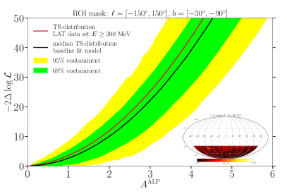
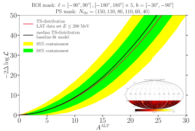
Figure 9: (Left:) TS-distribution with respect to the baseline fit model (based on Lorimer I; black) and its statistical scatter (green: 68$\%$ containment, yellow: 95$\%$ containment) as well as the TS distribution with respect to the 12-year Fermi-LAT data including energies above 200 MeV (red). (Right:) Same as the left panel with respect to the LAT data set of events with $E\leq 200$ MeV. The fitting procedure uses six macro energy bins. In the lower right corner of each panel we display the optimized ROI showing the total gamma-ray counts in the respective data set projected on the sky.

V.2 Upper limits on the ALP parameter space

After having determined in Sec. V.1 the ROI that yields the most statistically sound upper limits on the ALP signal, we are able to set upper limits on the normalization parameter $G_{a}$ of the signal template. Before that, we have checked that the selected parts of the sky do not contain a significant fraction of the ALP signal that would warrant a detection. We “unblind” our previous fitting routine by inserting the true signal template with the gamma-ray flux spectrum induced by ALPs from core-collapse SNe, Sec. III.2; hence, the re-introduction of the normalization parameter $G_{a}$.

In what follows, we consider and utilize a benchmark case of the DSNALPB gamma-ray spectrum to illustrate the upper limits on such a large-scale gamma-ray emission component. This benchmark model is defined by the following properties:

1. $f_{\rm fail-CC}=20\%$,

2. Salpeter IMF,

3. fiducial SNR description (see Tab. 2).

The uncertainty on the reported DSNALPB upper limits arising from varying these benchmark choices is discussed in Sec. VI. Therein, we also report the impact of altering the astrophysical surroundings of the Milky Way, that is, the employed IEM and GMF model.

We consider ALPs coupled only to photons. In this case, the upper limit on $G_{a}$ translates into an upper limit on the photon-ALP coupling strength via $g_{a\gamma}=\sqrt[4]{G_{a}}\,g_{a\gamma}^{\mathrm{ref}}$, where $g_{a\gamma}^{\mathrm{ref}}=5\times 10^{-12}\;\mathrm{GeV}^{-1}$ refers to the reference value of the coupling at which spectrum and ALP-photon conversion probability in the Milky Way have been calculated to obtained the ALP template.

In Fig. 10 we show the observed 95$\%$ CL upper limits (solid red line) on our benchmark DSNALPB scenario together with the expected statistical scatter ($68\%$ containment: green; $95\%$ containment: yellow) of the upper limits according to 250 Poisson realizations of the baseline gamma-ray sky model (cf. Sec. IV.2 for its derivation) whereas the solid black line denotes the median upper limit with respect to this baseline data set. The basis for the baseline sky model and all derived upper limits presented here are the ALP signal morphology due to the Jansson model Jansson and Farrar (2012) of the Milky Way’s GMF and the iteratively optimized IEM Lorimer I. We also confront the upper limits obtained in this analysis with existing limits on the ALP parameter space.

In this particular setting, we find an improvement of the upper limit on $g_{a\gamma}$ regarding our previous analysis in Paper I that was solely based on the spectral shape of the ALP-induced gamma-ray flux (and neglecting the effect of gravitational energy-redshift as well as the formation of alpha particles during a CC SN). Specifically, we obtain $g_{a\gamma}\lesssim 3.76\times 10^{-11}$ GeV^-1 for ALP masses $m_{a}\ll 10^{-11}$ eV at $95\%$ CL.

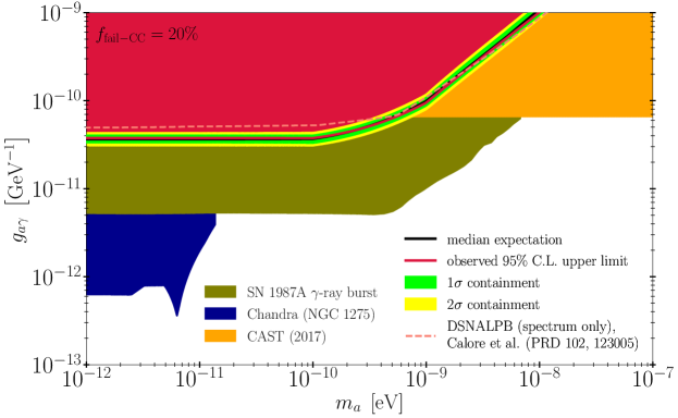
Figure 10: 95$\%$ CL upper limits (solid red) on the ALP-photon coupling constant $g_{a\gamma}$ assuming the benchmark DSNALPB scenario and an ALP coupling exclusively to photons as well as the ‘Jansson12c’ Adam et al. (2016b) model of the Milky Way’s GMF. The filled red region illustrates the ALP parameter space excluded by this upper limit. The displayed green (yellow) band reflects the expected $1\sigma\,(2\sigma)$ statistical scatter of the upper limits based on 250 Poisson realizations of the “mock data” obtained via the baseline fit of the gamma-ray sky. The solid black line represents the median upper limit obtained from these fits to mock data. To highlight the improvement on the upper limits set with the analysis in Paper I, which is solely based on the expected spectral shape of the DSNALPB gamma-ray flux, we show this result as a dashed, light-red line. Our results are complemented by independent astrophysical and helioscope bounds on the ALP-photon coupling strength from CAST Anastassopoulos et al. (2017), Chandra observations of NGC 1275 Reynolds et al. (2019) as well as the non-observation of a gamma-ray burst following SN 1987A Payez et al. (2015).

VI Discussion

This section is dedicated to a discussion of the sources of systematic uncertainties on the DSNALPB upper limits reported in Sec. V. These uncertainties arise by varying the benchmark scenario decisions as well as the description of the astrophysical surroundings in the Milky Way.

While a number of dedicated explorations of particular sources of uncertainty regarding their impact on the ALP-photon coupling upper limits are given in App. B, we provide below in Tab. 5 a summary of the induced systematic uncertainty for the “massless” ALP case $m_{a}\ll 10^{-11}$ eV while always referring to the benchmark DSNALPB scenario as reference point.

source of uncertainty	absolute $\left[10^{-11}\;\mathrm{GeV}^{-1}\right]$	relative $\left[\%\right]$
$f_{\mathrm{fail-CC}}$	$\left[2.81,4.73\right]$	$51.1$
IMF	$\left[3.76,4.03\right]$	$7.2$
SNR	$\left[3.59,3.98\right]$	$10.4$
IEM	$\left[3.24,3.76\right]$	$13.8$
GMF model	$\left[3.76,5.22\right]$	$38.8$
total	$\left[2.38,7.04\right]$	$124$

Table 5: Induced uncertainty on the ALP-photon coupling constant $g_{a\gamma}$ with respect to varying the conditions and properties assumed in the benchmark DSNALPB scenario and $m_{a}\ll 10^{-11}$ eV. The last row indicates the total systematic uncertainty range when all sources of uncertainty are combined to form a most optimistic and most pessimistic scenario.

For each source of uncertainty – listed in the first column – we report in the second column the associated absolute uncertainty range of the derived $95\%$ CL upper limits. The stated absolute range quantifies the minimal and maximal constraint that we find by varying the respective quantity within its uncertainty range, while keeping all other quantities fixed to their values attained in the benchmark case. These boundaries do not need to be symmetric around the benchmark upper limit depending on the source of uncertainty. For example, we only consider one alternative GMF model so that the reported interval refers to the numbers obtained with respect to either the Jansson & Farrar model or the Pshirkov model. The third column of Tab. 5 contains the relative uncertainty taken with respect to the nominal value of the upper limit for the benchmark case. This means, we take the difference between the lower and upper boundary in the first column and divide it by the benchmark upper limit.

To be more explicit regarding the origin the table’s content, the $f_{\mathrm{fail-CC}}$ uncertainty range reflects the grey band in Fig. 6; the IMF uncertainty arises from the two alternative initial mass functions Kroupa and BG (see Sec. III.2); the SNR uncertainty uses the remaining parametrizations in Tab. 2, the IEM uncertainty range uses the five different models introduced in Sec. IV.2 and the GMF model uncertainty reflects the change from the Jansson & Farrar prescription to the Pshirkov model. This assessment of the systematic uncertainties of our upper bounds singles out the unknown fraction of failed CC SNe, as well as the strength and structure of the Milky Way’s GMF as the most significant drivers of uncertainty, contributing an error of about 51% and 39% respectively.
On the other hand, the uncertainty related to the IMF, SNR parametrization, and IEM account for a $\sim$ 10% relative error.

The values in the first lines of Tab. 5 provide an estimate of the uncertainty due to individual inputs since have been derived by varying only a single source of uncertainty at a time. To get an impression of the overall uncertainty we consider most optimistic and pessimistic scenarios that lead to the best or worst possible upper limits on the DSNALPB. The resulting systematic uncertainty band is displayed in Fig. 11. With respect to these most optimistic and pessimistic scenarios, the systematic uncertainties may allow the $95\%$ CL upper limit on the DSNALPB to be placed between $g_{a\gamma}\lesssim\left[2.38,7.04\right]\times 10^{-11}\;\mathrm{GeV}^{-1}$ in the case of massless ALPs.

Further details on the uncertainties can be found in App. B.

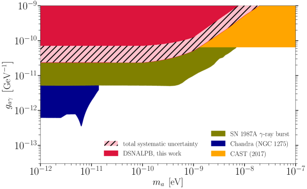
Figure 11: 95$\%$ CL upper limits (red band) on the ALP-photon coupling constant $g_{a\gamma}$ assuming a coupling exclusively to photons. The displayed pink hatched band reflects the total systematic uncertainty on the DSNALPB gamma-ray spectrum caused by combining all sources of uncertainty considered in this analysis (see Tab. 5) to form a most optimistic and a most pessimistic scenario. Our results are complemented by independent astrophysical and helioscope bounds on the ALP-photon coupling strength from CAST Anastassopoulos et al. (2017), Chandra observations of NGC 1275 Reynolds et al. (2019) as well as the non-observation of a gamma-ray burst following SN 1987A Payez et al. (2015).

VII Conclusions

In this work, we carried out a comprehensive analysis of the gamma-ray diffuse signal induced by axion-like particles (ALPs) produced by all past cosmic core-collaps supernovae (CC SNe) and converted into high-energy photons when experiencing the magnetic field of the Galaxy.

We presented a refined calculation of the ALPs flux from extragalactic SNe: we go beyond the simple approximation that the ALPs flux is independent on the SN mass progenitor by modeling the ALPs signal from different state-of-the-art SN models with progenitor masses between 8.8 and 70 $M_{\odot}$. Moreover, we accounted for the possibility that not all CC SNe lead to successful explosions, by quantifying the fraction of failed CC SN explosions and building the corresponding model for the ALPs signal upon two simulations of failed CC SN explosions.

We explored four different scenarios, each of them characterized by a different fraction of failed CC SN explosions, allowing us to quantify the uncertainty due to failed CC SN explosions. The calculation of the ALPs flux from all past cosmic SNe accounts also for uncertainties related to the cosmic SN rate.

Using this new model for the diffuse supernova ALP background (DSNALPB) gamma-ray flux, we run a systematic analysis of 12 years of data collected by -LAT with the aim of setting robust upper limits on the ALPs parameter space. For the first time in the context of ALPs searches, we performed a template-based gamma-ray analysis to fully exploit the spatial features of the ALPs signal. The flux from the DSNALPB being peaked at about 25 MeV, we exploited the full LAT data sets by developing an optimized low-energy ($E\lesssim 200$ MeV) analysis. Besides, we optimized the IEMs in a data-driven way and limit the impact of the IE mis-modeling on the final limits – which, indeed, are only mildly affected by changing the IEM. We also selected the ROI in order to be able to set statistically sound upper limit on the signal model.

Our final limits slightly improve the CAST bound (in the low mass region). However, they are still about a factor of six (regarding our baseline scenario) above the SN1987A gamma-ray burst limit. It is nevertheless a valuable confirmation, as they do not depend on a single event. More importantly, we quantified for the first time the width of the uncertainty band of the DSNALPB limit, which turns out to be less than a factor of three and dominated by the uncertainty on the fraction of failed CC SN explosions. A significant improvement on our bound would be therefore reached exploiting the synergies with the detection of the future diffuse supernova neutrino background (DSNB). Indeed, as pointed out in Ref. Møller et al. (2018), a combined detection of the DSNB in the next-generation neutrino detectors will be sensitive to the local supernova rate at a $\sim 33$ % level, and will give an uncertainty on the fraction of supernovae that form black holes that will be at most $\sim 0.4$. Consequently, the uncertainty on the DSNALPB flux would be significantly reduced.

Uncertainties on the IEM are sub-dominant, while those on the GMF remain an important source of systematic uncertainties for ALPs searches. In this respect, we stress that only the transversal component to the ALPs’ propagation is relevant for the conversion. Diffuse synchrotron in radio- and microwaves and thermal dust emission are crucial for constraining GMF models perpendicular to the line-of-sight, and complement each other. Improvements on our description of the GMF are expected by new radio- and microwave surveys (e.g. SKA, QUIJOTE), as well as from the synergy between GAIA and Planck through a detailed mapping of the dust distribution via extinction. SKA will also allow the scientific community to make a leap forward in the number of pulsars known in the Galaxy (and therefore in Faraday rotation data), and to refine our model for electron density and the parallel magnetic field component. A better comprehension of the Galactic cosmic-ray population from AMS-02 future measurements and gamma-ray telescopes, joint with synchrotron maps, will also help us constraining the GMF ordering. We refer the reader to Jaffe (2019) for a more detailed discussion and overview.

To conclude, we have presented here a first, systematic, analysis of the ALPs diffuse background from CC SNe with gamma-ray data, leveraging on the unique sensitivity of the -LAT.

Appendix A Details on the calculation of the ALP spectrum

A.1 Impact of the alpha particles

Usually the ALP Primakoff production in SN has been characterized including only the contributions from protons. However, as recently pointed out in Caputo et al. (2021) the contribution of alpha particles in the SN core might be non negligible. Indeed, we confirm that also for the SN models we use, there is a sizable gap between the proton abundance $Y_{p}$ and $1-Y_{n}$, as shown in Fig. 12, that we can assume to be filled by alpha particles.
In order to evaluate the effect of these particles on the ALP production, a reasonable choice according to Caputo et al. (2021) is to correct the inverse Debye screening length $\kappa$ described by

$$\kappa^{2}=\frac{4\pi\alpha\hat{n}}{T}\;,$$ (17)

where $\hat{n}=\sum_{j}Z_{j}^{2}n_{j}=\hat{Y}n_{\rm B}$, where $\hat{Y}$ is the effective charge per nucleon. If all nuclei heavier than protons were realized as $\alpha$ particles, we would have $X_{\alpha}+X_{n}+X_{p}=1$, where $X_{j}$ represents the mass fraction for the particle $j$. In this framework $\hat{Y}=Y_{p}+4X_{\alpha}/4=Y_{p}+X_{\alpha}$. The difference in the SN energy spectrum can be observed for the $25M_{\odot}$ SN progenitor is shown in Fig. 13. We find that the inclusion of alpha particles produces an enhancement of $\sim 15\%$ of the ALP flux.

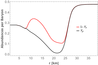
Figure 12: Charged particles abundances a $t_{\textrm{pb}}=1$ s for the model $M=25\,M_{\odot}$.

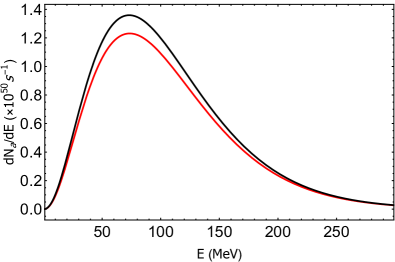
Figure 13: Comparison beetween produced SN ALP number flux as a function of energy taking into account the Primakoff production only from protons (red line) and including also the production from $\alpha$ particles (black line). The chosen model is the $M=25\,M_{\odot}$. We assume $g_{a\gamma}=10^{-11}\operatorname{GeV}^{-1}$.

A.2 Gravitational energy-redshift

The ALPs emission is affected by the gravitational field of the neutron star, in particular time dilation, trajectory bending and the red-shifting of the energy. In this appendix we discuss the implementation of these gravitational effects in our analysis.

Let us start with a couple of general comments. We are calculating the time integrated production in the local reference frame. As we are not interested in the time dependence of the signal, particle number conservation ensures that we have the correct number of ALPs also outside the supernova. As we are considering an isotropic flux, trajectory bending can be ignored. The most important effect for us is the red-shift of the energy, because it directly affects the spectrum which in turn determines the sensitivity of Fermi-LAT.

All SN simulations discussed in the present manuscript are based on general relativistic neutrino radiation hydrodynamics Liebendörfer et al. (2004); Kuroda et al. (2018, 2021), i.e. the metric functions are obtained through direct numerical integration of the Einstein field equations for a given line element, $ds^{2}=g_{\alpha\beta}dx^{\alpha}dx^{\beta}$. The zeroth component, known as the lapse function, $g_{00}=-\exp\{2\Phi\}$, determines the gravitational red(blue) shifting of the axion energy as follows,

$$E=E^{*}(x)\,\textrm{exp}(\Phi(x))\;,$$ (18)

with the lapse function being evaluated locally at the PNS interior, depending on the choice of the coordinate system $\{x^{\alpha}\}$, relating the ALP energy $E$ measured by an observer at infinity with the local ALP energy $E^{*}(x)$. Similarly, for a local observer, time dilation must be taken into account as follows

$$dt=dt^{*}(x)\,\ \textrm{exp}(\Phi(x))\;,$$ (19)

where the $dt^{*}(x)$ refers to the local observer time at $x$, while $dt$ refers to the simulation time corresponding to that of a distant observer.

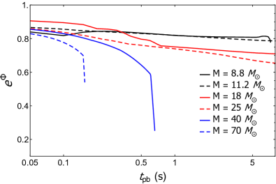
Figure 14: Post-bounce evolution of the lapse function $e^{\Phi}$ sampled at a distance from the center of $r=5$ km for different SN simulations under investigation.

In Figure 14, we show the time evolution of the lapse function $e^{\Phi}$ for the different SN progenitors at a distance from the center of $r=5$ km. We note that for exploding SNe this factor decreases monotonically in time, the effect being larger for higher progenitor masses, and ranging between 0.7–0.8. For failed SN collapsing to black-holes, the gravitational effect is larger, i.e. the lapse function is dropping to $\sim 0.5$ for the $70$ $M_{\odot}$ progenitor already shortly after core bounce and below $0.01$ when the apparent horizon appears at $t_{\rm pb}\sim 0.155$ s (Kuroda et al., 2021).

The ALP Primakoff production rate of Eq. (2) in terms of the local quantities reads

$$\frac{d{n}_{\rm a}}{dE^{*}dt^{*}}=\frac{g_{\rm a\gamma}^{2}\xi^{2}T^{3}(E^{*})^{3}}{8\pi^{3}(e^{E^{*}/T-1})}\biggl{[}\frac{\xi^{2}T^{2}}{(E^{*})^{2}}\textrm{ln}\biggl{(}1+\frac{(E^{*})^{2}}{\xi^{2}T^{2}}\biggr{)}\biggr{]}.$$ (20)

Since $dE^{*}dt^{*}=dE\,\ dt$, the redshifted time-integrated ALP spectrum at infinity is given by

$$\frac{dN_{\rm a}}{dE} = \int d^{3}rdt\frac{d{n}_{\rm a}}{dEdt}$$ (21)

$$= \int d^{3}rdt^{*}\frac{d{n}_{\rm a}}{dE^{*}dt^{*}}\textrm{exp}(-\Phi(r))\,\ .$$

As shown in Sec. III, the ALP spectrum can be fitted by the following functional form

$$\frac{dN_{a}}{dE}=C\left(\frac{g_{a\gamma}}{10^{-11}\textrm{GeV}^{-1}}\right)^{2}\left(\frac{E}{E_{0}}\right)^{\beta}\exp\left(-\frac{(\beta+1)E}{E_{0}}\right)\,.$$ (22)

In Table 6, we compare the fitting parameters of Eq. (22) without and with gravitational energy-redshift, respectively for different progenitor masses. We see that the effect of gravitational energy-redsfhit is to reduce the average energy of the spectrum $E_{0}$ and increase the normalization parameter $c$ to compensate the drop in $E_{0}$. The effect of drop of the energy increases monotonically in function of the SN progenitor mass, ranging from $\sim 20\%$ for 8.8 $M_{\odot}$ progenitor to $360\%$ for 70 $M_{\odot}$. Indeed, increasing the progenitor mass we increase the gravitational potential, especially for the high-mass progenitor cases ending into a black-hole. The effect on the $C$ parameter is milder, the increase being at most $\sim 30\%$. The factor $\beta$ being given by

$$\frac{\langle E^{2}\rangle-\langle E\rangle^{2}}{\langle E\rangle^{2}}=\frac{1}{1+\beta}\,\ ,$$ (23)

is rather insensitive to the effect of the redshift.

Table 6: Fitting parameters for the SN ALP spectrum, Eq. 22, from the Primakoff process for different SN progenitors estimated for $g_{a\gamma}=10^{-11}\,\textrm{GeV}^{-1}$ and $m_{a}\ll 10^{-11}$ eV, assuming no gravitational energy-redshift/accounting for the gravitational redshift. $\alpha$ particles contribution to the Primakoff production is included.

SN progenitor	$C$ [$\times 10^{50}\,\ {\rm MeV}^{-1}$]	$E_{0}$ [MeV]	$\beta$
8.8 $M_{\odot}$	$4.18/4.81\,\$	90.62/78.15	2.56/2.60
11.2 $M_{\odot}$	$6.25/8.11\,\$	91.81/76.04	2.74/2.80
18 $M_{\odot}$	$18.4/26.1\,\$	119.4/89.32	2.40/2.45
25 $M_{\odot}$	$21.0/31.1\,\$	145.4/104.9	2.25/2.30
40 $M_{\odot}$	$1.56/2.98\,\$	168.9/110.6	1.77/1.94
70 $M_{\odot}$	$0.131/0.213\,\$	127.5/94.36	1.13/1.76

Table 7: Fitting parameters for DSNALPB fluxes for $g_{a\gamma}=10^{-11}$ GeV^-1 and $m_{a}\ll 10^{-11}$ eV for different fractions of failed SNe $f_{\rm fail-CC}$, without gravitational energy-redshift/accounting for the gravitational redshift. $\alpha$ particles contribution to the Primakoff production is included.

$f_{\textrm{fail-CC}}$	$C$	$E_{0}$	$\beta$
	[$\times 10^{-7}{\rm MeV}^{-1}\textrm{cm}^{-2}\textrm{s}^{-1}$]	[MeV]
10% max flux	$96.2/144\,\$	58.5/43.8	1.39/1.50
10%	$58.0/88.9\,\$	59.3/43.5	1.32/1.42
20%	$42.9/62.9\,\$	52.0/39.9	1.41/1.49
30%	$31.0/46.5\,\$	50.8/39.3	1.37/1.47
40%	$22.4/35.8\,\$	52.7/40.2	1.28/1.41
40% min flux	$9.33/15.7\,\$	57.6/42.3	1.17/1.32

In order to quantify the impact of the gravitational energy-redshift on the DSNALPB spectrum, we show the variation of the fitting parameters of Eq. 22 in Table 7, neglecting and including the gravitational energy-redshift effect, respectively. We realize that the effect of gravitational energy-redshift is the same observed on the spectrum of a single SN, i.e. increase of the normalization factor $C$ and decrease in the average energy $E_{0}$. The effect of the corrections on both parameters ranges between $\sim 25-35\%$. We remark that the effect of the gravitational redshift is more sizable for failed SNe, which are never dominant in the DSNALPB flux, contributing at most at $40\%$ of the SN progenitors. This would somehow dilute the final impact of the gravitational energy-redshift on the DSNALPB spectrum.

Appendix B Systematic uncertainty on the DSNALPB upper limits of cosmological and astrophysical origin

The following subsections contain a more detailed discussion of some of the sources of uncertainty regarding their impact on the ALP-photon coupling upper limits for the entirety of the relevant ALP mass range complementing the content of Tab. 5.

B.1 Impact of the fraction of failed CC SNe

As can be seen from the last column of Tab. 5, the uncertainty of the fraction of failed CC SNe in the progenitor mass range chosen to compute the DSNALPB is the most important source of systematic uncertainty for this type of ALP-induced gamma-ray signal.

In Fig. 15, we show the uncertainty band due to this source of systematic error in the full parameter space of ALPs.

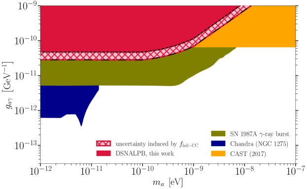
Figure 15: 95$\%$ CL upper limits (red band) on the ALP-photon coupling constant $g_{a\gamma}$ assuming a coupling exclusively to photons and the ‘Jansson12c’ Adam et al. (2016b) model of the Milky Way’s GMF. The displayed band reflects the uncertainty on the DSNALPB gamma-ray spectrum caused by the unknown ratio of failed to successful CCSNe within the mass range of SN progenitors considered in this analysis (see Sec. III.2) while keeping all other properties as in the benchmark scenario. Our results are complemented by independent astrophysical and helioscope bounds on the ALP-photon coupling strength from CAST Anastassopoulos et al. (2017), Chandra observations of NGC 1275 Reynolds et al. (2019) as well as the non-observation of a gamma-ray burst following SN 1987A Payez et al. (2015).

B.2 Impact of the Galactic magnetic field model

To assess the robustness of the upper limits presented in Sec. V against different assumptions and models of the Milky Way’s magnetic field, we create a sample of alternative signal templates which have been taken from a recent study of the planck collaboration Adam et al. (2016b) (Tab. 3.1 therein) and Pshirkov et al. (2011).

A comparison of the upper limits obtained from these models is displayed in Fig. 16. In general, different GMF models induce a variation in the derived upper limits on $g_{a\gamma}$ of $\mathcal{O}(1)$ whose relative impact on the final upper limit is comparable to the one of the $f_{\mathrm{fail-CC}}$ parameter according to Tab. 5.

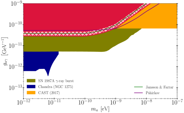
Figure 16: As in Fig. 15. However, here we focus on the variation with respect to the magnetic field model. We confront the upper limits derived with different characterisations of the Milky Way’s magnetic field; ‘Jansson12c’ Adam et al. (2016b) (green) and ‘Pshirkov’ Pshirkov et al. (2011) (purple). For comparison, the theoretical uncertainty due to the fraction of failed and successful CC SNe is shown as a light red band.

B.3 Impact of the Galactic diffuse foreground model

Although the ROI optimising has been conducted in the high-latitude gamma-ray sky to minimize the contamination by the Milky Way’s diffuse foreground emission, we investigate the robustness of the upper limits shown in Sec. V against variations of the Galactic foreground. To this end, we re-run the analysis pipeline with respect to the alternative IEMs introduced in Sec. IV.2.

The results of this cross-check are presented in Fig. 17. Variations of the IE have a smaller impact than model uncertainties in the magnetic field of the Milky Way. On one side, this implies that our analysis pipeline is robust against such alterations while, on the other side, it is essential to improve the existing models of the GMF, in particular, at high-latitudes.

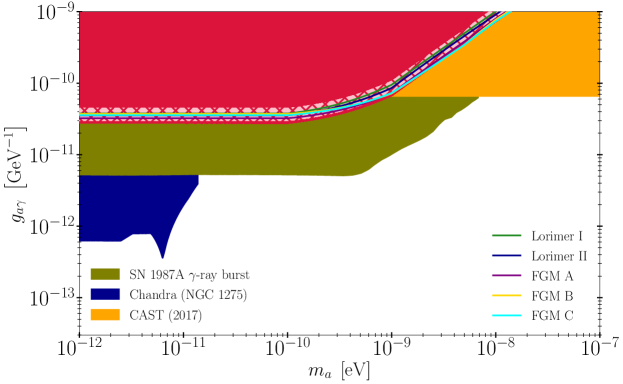
Figure 17: As in Fig. 15 but here we focus on the dependence with respect to the background model. We compare the upper limits derived with our benchmark choice of IEM ‘Lorimer I’ (green) with four alternative IEMs (c.f. Sec. IV.2). Again, for comparison, the theoretical uncertainty due to the fraction of failed and successful CC SNe is shown as a light red band.

References

- Eckner et al. (2021) C. Eckner, F. Calore, P. Carenza, et al., “Constraining the diffuse supernova axion-like-particle background with high-latitude Fermi-LAT data,” in Proceedings of 37th International Cosmic Ray Conference — PoS(ICRC2021), Vol. 395 (2021) p. 543.
- Agrawal et al. (2021) P. Agrawal et al., “Feebly-Interacting Particles:FIPs 2020 Workshop Report,” (2021), arXiv:2102.12143 [hep-ph].
- Raffelt (1996) G. G. Raffelt, Stars as laboratories for fundamental physics: The astrophysics of neutrinos, axions, and other weakly interacting particles (1996).
- Raffelt (2008) G. G. Raffelt, “Astrophysical axion bounds,” Lect. Notes Phys. 741, 51 (2008), arXiv:hep-ph/0611350.
- Fischer et al. (2016) T. Fischer, S. Chakraborty, M. Giannotti, et al., “Probing axions with the neutrino signal from the next galactic supernova,” Phys. Rev. D 94, 085012 (2016), arXiv:1605.08780 [astro-ph.HE].
- Brockway et al. (1996) J. W. Brockway, E. D. Carlson, and G. G. Raffelt, “SN1987A gamma-ray limits on the conversion of pseudoscalars,” Phys. Lett. B 383, 439 (1996), arXiv:astro-ph/9605197.
- Grifols et al. (1996) J. A. Grifols, E. Masso, and R. Toldra, “Gamma-rays from SN1987A due to pseudoscalar conversion,” Phys. Rev. Lett. 77, 2372 (1996), arXiv:astro-ph/9606028.
- Carenza et al. (2019) P. Carenza, T. Fischer, M. Giannotti, et al., “Improved axion emissivity from a supernova via nucleon-nucleon bremsstrahlung,” JCAP 10, 016 (2019), [Erratum: JCAP 05, E01 (2020)], arXiv:1906.11844 [hep-ph].
- Lucente et al. (2020) G. Lucente, P. Carenza, T. Fischer, et al., “Heavy axion-like particles and core-collapse supernovae: constraints and impact on the explosion mechanism,” JCAP 12, 008 (2020), arXiv:2008.04918 [hep-ph].
- Payez et al. (2015) A. Payez, C. Evoli, T. Fischer, et al., “Revisiting the SN1987A gamma-ray limit on ultralight axion-like particles,” JCAP 02, 006 (2015), arXiv:1410.3747 [astro-ph.HE].
- Dessert et al. (2020) C. Dessert, J. W. Foster, and B. R. Safdi, “X-ray Searches for Axions from Super Star Clusters,” Phys. Rev. Lett. 125, 261102 (2020), arXiv:2008.03305 [hep-ph].
- Meyer et al. (2017) M. Meyer, M. Giannotti, A. Mirizzi, et al., “Fermi Large Area Telescope as a Galactic Supernovae Axionscope,” Phys. Rev. Lett. 118, 011103 (2017), arXiv:1609.02350 [astro-ph.HE].
- Meyer and Petrushevska (2020) M. Meyer and T. Petrushevska, “Search for Axionlike-Particle-Induced Prompt -Ray Emission from Extragalactic Core-Collapse Supernovae with the Large Area Telescope,” Phys. Rev. Lett. 124, 231101 (2020), [Erratum: Phys.Rev.Lett. 125, 119901 (2020)], arXiv:2006.06722 [astro-ph.HE].
- Meyer and Petrushevska (2021) M. Meyer and T. Petrushevska (Fermi-LAT), “Extending the sample of core-collapse supernovae for searches of axion-like-particle induced gamma-ray bursts with the Fermi LAT,” PoS ICRC2021, 510 (2021), arXiv:2108.02069 [astro-ph.HE].
- Crnogorčević et al. (2021) M. Crnogorčević, R. Caputo, M. Meyer, et al., “Searching for Axion-Like Particles from Core-Collapse Supernovae with Fermi LAT’s Low Energy Technique,” (2021), arXiv:2109.05790 [astro-ph.HE].
- Diehl et al. (2006) R. Diehl, H. Halloin, K. Kretschmer, et al., “Radioactive 26Al from massive stars in the Galaxy,” Nature (London) 439, 45 (2006), arXiv:astro-ph/0601015 [astro-ph].
- Raffelt et al. (2011) G. G. Raffelt, J. Redondo, and N. Viaux Maira, “The meV mass frontier of axion physics,” Phys. Rev. D 84, 103008 (2011), arXiv:1110.6397 [hep-ph].
- Calore et al. (2020) F. Calore, P. Carenza, M. Giannotti, et al., “Bounds on axionlike particles from the diffuse supernova flux,” Phys. Rev. D 102, 123005 (2020), arXiv:2008.11741 [hep-ph].
- Mattox et al. (1996) J. R. Mattox et al., “The Likelihood Analysis of EGRET Data,” Astrophys. J. 461, 396 (1996).
- Su et al. (2010) M. Su, T. R. Slatyer, and D. P. Finkbeiner, “Giant Gamma-ray Bubbles from Fermi-LAT: Active Galactic Nucleus Activity or Bipolar Galactic Wind?” Astrophys. J. 724, 1044 (2010), arXiv:1005.5480 [astro-ph.HE].
- Ackermann et al. (2012) M. Ackermann et al., “Constraints on the Galactic Halo Dark Matter from Fermi-LAT Diffuse Measurements,” Astrophys. J. 761, 91 (2012), arXiv:1205.6474 [astro-ph.CO].
- Ackermann et al. (2017) M. Ackermann et al. (Fermi-LAT), “The Fermi Galactic Center GeV Excess and Implications for Dark Matter,” Astrophys. J. 840, 43 (2017), arXiv:1704.03910 [astro-ph.HE].
- Storm et al. (2017) E. Storm, C. Weniger, and F. Calore, “SkyFACT: High-dimensional modeling of gamma-ray emission with adaptive templates and penalized likelihoods,” JCAP 08, 022 (2017), arXiv:1705.04065 [astro-ph.HE].
- Di Mauro et al. (2019) M. Di Mauro, X. Hou, C. Eckner, et al., “Search for -ray emission from dark matter particle interactions from Andromeda and Triangulum Galaxies with the Fermi Large Area Telescope,” Phys. Rev. D 99, 123027 (2019), arXiv:1904.10977 [astro-ph.HE].
- Di (2021) M. Di, “Characteristics of the Galactic Center excess measured with 11 years of -LAT data,” Phys. Rev. D 103, 063029 (2021), arXiv:2101.04694 [astro-ph.HE].
- Mezzacappa and Bruenn (1993) A. Mezzacappa and S. Bruenn, “A numerical method for solving the neutrino Boltzmann equation coupled to spherically symmetric stellar core collapse,” Astrophys. J. 405, 669 (1993).
- Liebendörfer et al. (2004) M. Liebendörfer, O. Messer, A. Mezzacappa, et al., “A Finite difference representation of neutrino radiation hydrodynamics for spherically symmetric general relativistic supernova simulations,” Astrophys. J. Suppl. 150, 263 (2004).
- Fischer (2016) T. Fischer, “The role of medium modifications for neutrino-pair processes from nucleon-nucleon bremsstrahlung. Impact on the protoneutron star deleptonization,” Astron. Astrophys. 593, A103 (2016).
- Fischer et al. (2020) T. Fischer, G. Guo, A. A. Dzhioev, et al., “Neutrino signal from proto-neutron star evolution: Effects of opacities from charged-current-neutrino interactions and inverse neutron decay,” Phys. Rev. C 101, 025804 (2020).
- Kuroda et al. (2021) T. Kuroda, T. Fischer, T. Takiwaki, and K. Kotake, “Core-collapse supernova simulations and the formation of neutron stars, hybrid stars, and black holes,” arXiv e-prints , arXiv:2109.01508 (2021), arXiv:2109.01508 [astro-ph.HE].
- Kotake et al. (2018) K. Kotake, T. Takiwaki, T. Fischer, et al., “Impact of Neutrino Opacities on Core-collapse Supernova Simulations,” Astrophys. J. 853, 170 (2018).
- Lattimer and Swesty (1991) J. M. Lattimer and F. Swesty, “A Generalized equation of state for hot, dense matter,” Nucl.Phys. A535, 331 (1991).
- Shen et al. (1998) H. Shen, H. Toki, K. Oyamatsu, and K. Sumiyoshi, “Relativistic equation of state of nuclear matter for supernova and neutron star,” Nucl.Phys. A637, 435 (1998).
- Hempel and Schaffner-Bielich (2010) M. Hempel and J. Schaffner-Bielich, “Statistical Model for a Complete Supernova Equation of State,” Nucl.Phys. A837, 210 (2010).
- Hempel et al. (2012) M. Hempel, T. Fischer, J. Schaffner-Bielich, and M. Liebendörfer, “New Equations of State in Simulations of Core-collapse Supernovae,” Astrophys. J. 748, 70 (2012).
- Steiner et al. (2013) A. W. Steiner, M. Hempel, and T. Fischer, “Core-collapse Supernova Equations of State Based on Neutron Star Observations,” Astrophys. J. 774, 17 (2013).
- Nomoto (1987) K. Nomoto, “Evolution of 8-10 solar mass stars toward electron capture supernovae. II - Collapse of an O + NE + MG core,” Astrophys. J. 322, 206 (1987).
- Kitaura et al. (2006) F. Kitaura, H.-T. Janka, and W. Hillebrandt, “Explosions of o-ne-mg cores, the crab supernova, and subluminous type ii-p supernovae,” Astron.Astrophys. 450, 345 (2006).
- Fischer et al. (2010) T. Fischer, S. Whitehouse, A. Mezzacappa, et al., “Protoneutron star evolution and the neutrino driven wind in general relativistic neutrino radiation hydrodynamics simulations,” Astron.Astrophys. 517, A80 (2010).
- Woosley et al. (2002) S. E. Woosley, A. Heger, and T. A. Weaver, “The evolution and explosion of massive stars,” Rev. Mod. Phys. 74, 1015 (2002).
- Baumgarte et al. (1996) T. Baumgarte, S. Teukolsky, S. Shapiro, et al., “Delayed collapse of hot neutron stars to black holes via hadronic phase transitions,” Astrophys.J. 468, 823 (1996).
- Sumiyoshi et al. (2006) K. Sumiyoshi, S. Yamada, H. Suzuki, and S. Chiba, “Neutrino signals from the formation of black hole: A probe of equation of state of dense matter,” Phys.Rev.Lett. 97, 091101 (2006), arXiv:astro-ph/0608509 [astro-ph].
- Fischer et al. (2009) T. Fischer, S. C. Whitehouse, A. Mezzacappa, et al., “The neutrino signal from protoneutron star accretion and black hole formation,” Astron. Astrophys. 499, 1 (2009).
- O’Connor and Ott (2011) E. O’Connor and C. D. Ott, “Black Hole Formation in Failing Core-Collapse Supernovae,” Astrophys. J. 730, 70 (2011), arXiv:1010.5550 [astro-ph.HE].
- Fischer et al. (2018) T. Fischer, N.-U. F. Bastian, M.-R. Wu, et al., “Quark deconfinement as a supernova explosion engine for massive blue supergiant stars,” Nat. Astron. 2, 980 (2018).
- Fischer (2021) T. Fischer, “QCD phase transition drives supernova explosion of a very massive star,” arXiv e-prints , arXiv:2108.00196 (2021), arXiv:2108.00196 [astro-ph.HE].
- Takahashi et al. (2014) K. Takahashi, H. Umeda, and T. Yoshida, “Stellar Yields of Rotating First Stars. I. Yields of Weak Supernovae and Abundances of Carbon-enhanced Hyper-metal-poor Stars,” Astrophys. J. 794, 40 (2014), arXiv:1406.5305 [astro-ph.SR].
- Kuroda et al. (2018) T. Kuroda, K. Kotake, T. Takiwaki, and F.-K. Thielemann, “A full general relativistic neutrino radiation-hydrodynamics simulation of a collapsing very massive star and the formation of a black hole,” Mon. Not. Roy. Astron. Soc. 477, L80 (2018), arXiv:1801.01293 [astro-ph.HE].
- Shibagaki et al. (2021) S. Shibagaki, T. Kuroda, K. Kotake, and T. Takiwaki, “Characteristic time variability of gravitational-wave and neutrino signals from three-dimensional simulations of non-rotating and rapidly rotating stellar core collapse,” Mon. Not. Roy. Astron. Soc. 502, 3066 (2021), arXiv:2010.03882 [astro-ph.HE].
- Raffelt and Stodolsky (1988) G. Raffelt and L. Stodolsky, “Mixing of the Photon with Low Mass Particles,” Phys. Rev. D 37, 1237 (1988).
- Raffelt (1986) G. G. Raffelt, “ASTROPHYSICAL AXION BOUNDS DIMINISHED BY SCREENING EFFECTS,” Phys. Rev. D 33, 897 (1986).
- Beacom (2010) J. F. Beacom, “The Diffuse Supernova Neutrino Background,” Ann. Rev. Nucl. Part. Sci. 60, 439 (2010), arXiv:1004.3311 [astro-ph.HE].
- Caputo et al. (2021) A. Caputo, G. Raffelt, and E. Vitagliano, “Muonic Boson Limits: Supernova Redux,” (2021), arXiv:2109.03244 [hep-ph].
- Horiuchi et al. (2009) S. Horiuchi, J. F. Beacom, and E. Dwek, “The Diffuse Supernova Neutrino Background is detectable in Super-Kamiokande,” Phys. Rev. D 79, 083013 (2009), arXiv:0812.3157 [astro-ph].
- Salpeter (1955) E. E. Salpeter, “The Luminosity function and stellar evolution,” Astrophys. J. 121, 161 (1955).
- Kroupa (2001) P. Kroupa, “On the variation of the initial mass function,” Mon. Not. Roy. Astron. Soc. 322, 231 (2001), arXiv:astro-ph/0009005.
- Baldry and Glazebrook (2003) I. K. Baldry and K. Glazebrook, “Constraints on a universal IMF from UV to near-IR galaxy luminosity densities,” Astrophys. J. 593, 258 (2003), arXiv:astro-ph/0304423.
- Gutcke and Springel (2019) T. A. Gutcke and V. Springel, “Simulating a metallicity-dependent initial mass function: consequences for feedback and chemical abundances,” Mon. Not. Roy. Astron. Soc. 482, 118 (2019), arXiv:1710.04222 [astro-ph.GA].
- Kresse et al. (2021) D. Kresse, T. Ertl, and H.-T. Janka, “Stellar Collapse Diversity and the Diffuse Supernova Neutrino Background,” Astrophys. J. 909, 169 (2021), arXiv:2010.04728 [astro-ph.HE].
- Møller et al. (2018) K. Møller, A. M. Suliga, I. Tamborra, and P. B. Denton, “Measuring the supernova unknowns at the next-generation neutrino telescopes through the diffuse neutrino background,” JCAP 05, 066 (2018), arXiv:1804.03157 [astro-ph.HE].
- Pejcha and Thompson (2015) O. Pejcha and T. A. Thompson, “The Landscape of the Neutrino Mechanism of Core-Collapse Supernovae: Neutron Star and Black Hole Mass Functions, Explosion Energies and Nickel Yields,” Astrophys. J. 801, 90 (2015), arXiv:1409.0540 [astro-ph.HE].
- Ertl et al. (2016) T. Ertl, H. T. Janka, S. E. Woosley, et al., “A two-parameter criterion for classifying the explodability of massive stars by the neutrino-driven mechanism,” Astrophys. J. 818, 124 (2016), arXiv:1503.07522 [astro-ph.SR].
- Raithel et al. (2018) C. A. Raithel, T. Sukhbold, and F. Özel, “Confronting Models of Massive Star Evolution and Explosions with Remnant Mass Measurements,” Astrophys. J. 856, 35 (2018), arXiv:1712.00021 [astro-ph.HE].
- Sukhbold et al. (2016) T. Sukhbold, T. Ertl, S. E. Woosley, et al., “Core-Collapse Supernovae from 9 to 120 Solar Masses Based on Neutrino-powered Explosions,” Astrophys. J. 821, 38 (2016), arXiv:1510.04643 [astro-ph.HE].
- Hidaka et al. (2016) J. Hidaka, T. Kajino, and G. J. Mathews, “Red-supergiant and Supernova Rate Problems: Implication for the Relic Supernova Neutrino Spectrum,” Astrophys. J. 827, 85 (2016).
- Adams et al. (2017) S. M. Adams, C. S. Kochanek, J. R. Gerke, and K. Z. Stanek, “The search for failed supernovae with the Large Binocular Telescope: constraints from 7 yr of data,” Mon. Not. Roy. Astron. Soc. 469, 1445 (2017), arXiv:1610.02402 [astro-ph.SR].
- Fischer et al. (2020) T. Fischer, M.-R. Wu, B. Wehmeyer, et al., “Core-collapse Supernova Explosions Driven by the Hadron-quark Phase Transition as a Rare -process Site,” Astrophys. J. 894, 9 (2020), arXiv:2003.00972 [astro-ph.HE].
- Lunardini (2016) C. Lunardini, “Diffuse supernova neutrinos at underground laboratories,” Astropart. Phys. 79, 49 (2016), arXiv:1007.3252 [astro-ph.CO].
- Yuksel et al. (2008) H. Yuksel, M. D. Kistler, J. F. Beacom, and A. M. Hopkins, “Revealing the High-Redshift Star Formation Rate with Gamma-Ray Bursts,” Astrophys. J. Lett. 683, L5 (2008), arXiv:0804.4008 [astro-ph].
- Hopkins and Beacom (2006) A. M. Hopkins and J. F. Beacom, “On the normalisation of the cosmic star formation history,” Astrophys. J. 651, 142 (2006), arXiv:astro-ph/0601463.
- Horns et al. (2012) D. Horns, L. Maccione, M. Meyer, et al., “Hardening of TeV gamma spectrum of AGNs in galaxy clusters by conversions of photons into axion-like particles,” Phys. Rev. D 86, 075024 (2012), arXiv:1207.0776 [astro-ph.HE].
- Jaffe (2019) T. R. Jaffe, “Practical Modeling of Large-Scale Galactic Magnetic Fields: Status and Prospects,” Galaxies 7, 52 (2019), arXiv:1904.12689 [astro-ph.GA].
- Jansson and Farrar (2012) R. Jansson and G. R. Farrar, “A New Model of the Galactic Magnetic Field,” Astrophys. J. 757, 14 (2012), arXiv:1204.3662 [astro-ph.GA].
- Adam et al. (2016a) R. Adam et al. (Planck), “Planck intermediate results.: XLII. Large-scale Galactic magnetic fields,” Astron. Astrophys. 596, A103 (2016a), arXiv:1601.00546 [astro-ph.GA].
- Kleimann et al. (2019) J. Kleimann, T. Schorlepp, L. Merten, and J. Becker Tjus, “Solenoidal Improvements for the JF12 Galactic Magnetic Field Model,” Astrophys. J. 877, 76 (2019), arXiv:1809.07528 [astro-ph.GA].
- Pshirkov et al. (2011) M. S. Pshirkov, P. G. Tinyakov, P. P. Kronberg, and K. J. Newton-McGee, “Deriving global structure of the Galactic Magnetic Field from Faraday Rotation Measures of extragalactic sources,” Astrophys. J. 738, 192 (2011), arXiv:1103.0814 [astro-ph.GA].
- Cordes and Lazio (2002) J. M. Cordes and T. J. W. Lazio, “NE2001. 1. A New model for the galactic distribution of free electrons and its fluctuations,” (2002), arXiv:astro-ph/0207156.
- Górski et al. (2005) K. M. Górski, E. Hivon, A. J. Banday, et al., “HEALPix: A Framework for High-Resolution Discretization and Fast Analysis of Data Distributed on the Sphere,” ApJ 622, 759 (2005), arXiv:astro-ph/0409513 [astro-ph].
- Cowan et al. (2011) G. Cowan, K. Cranmer, E. Gross, and O. Vitells, “Asymptotic formulae for likelihood-based tests of new physics,” Eur. Phys. J. C 71, 1554 (2011), [Erratum: Eur.Phys.J.C 73, 2501 (2013)], arXiv:1007.1727 [physics.data-an].
- Acero et al. (2016) F. Acero et al. (Fermi-LAT), “The First Fermi LAT Supernova Remnant Catalog,” Astrophys. J. Suppl. 224, 8 (2016), arXiv:1511.06778 [astro-ph.HE].
- Lorimer et al. (2006) D. R. Lorimer et al., “The Parkes multibeam pulsar survey: VI. Discovery and timing of 142 pulsars and a Galactic population analysis,” Mon. Not. Roy. Astron. Soc. 372, 777 (2006), arXiv:astro-ph/0607640.
- Ackermann et al. (2015) M. Ackermann et al. (Fermi-LAT), “The spectrum of isotropic diffuse gamma-ray emission between 100 MeV and 820 GeV,” Astrophys. J. 799, 86 (2015), arXiv:1410.3696 [astro-ph.HE].
- Abdollahi et al. (2020) S. Abdollahi et al. (Fermi-LAT), “ Large Area Telescope Fourth Source Catalog,” Astrophys. J. Suppl. 247, 33 (2020), arXiv:1902.10045 [astro-ph.HE].
- Ballet et al. (2020) J. Ballet, T. H. Burnett, S. W. Digel, and B. Lott (Fermi-LAT), “Fermi Large Area Telescope Fourth Source Catalog Data Release 2,” (2020), arXiv:2005.11208 [astro-ph.HE].
- Herold and Malyshev (2019) L. Herold and D. Malyshev, “Hard and bright gamma-ray emission at the base of the Fermi bubbles,” Astron. Astrophys. 625, A110 (2019), arXiv:1904.01454 [astro-ph.HE].
- Wolleben (2007) M. Wolleben, “A New Model For The Loop-I (The North Polar Spur) Region,” Astrophys. J. 664, 349 (2007), arXiv:0704.0276 [astro-ph].
- Johannesson and Orlando (2013) G. Johannesson and E. Orlando, “Accounting for the Sun and the Moon in Fermi-LAT Analysis,” in International Cosmic Ray Conference, International Cosmic Ray Conference, Vol. 33 (2013) p. 3106, arXiv:1307.0197 [astro-ph.IM].
- Macias et al. (2019) O. Macias, S. Horiuchi, M. Kaplinghat, et al., “Strong Evidence that the Galactic Bulge is Shining in Gamma Rays,” JCAP 09, 042 (2019), arXiv:1901.03822 [astro-ph.HE].
- Dembinski et al. (2020) H. Dembinski, P. Ongmongkolkul, C. Deil, et al., “scikit-hep/iminuit: v1.5.2,” (2020), 10.5281/zenodo.4047970.
- Zechlin et al. (2018) H.-S. Zechlin, S. Manconi, and F. Donato, “Constraining Galactic dark matter with gamma-ray pixel counts statistics,” Phys. Rev. D 98, 083022 (2018), arXiv:1710.01506 [astro-ph.HE].
- Jansson and Farrar (2012) R. Jansson and G. R. Farrar, “A New Model of the Galactic Magnetic Field,” Astrophys. J. 757, 14 (2012), arXiv:1204.3662 [astro-ph.GA].
- Adam et al. (2016b) R. Adam et al. (Planck), “Planck intermediate results.: XLII. Large-scale Galactic magnetic fields,” Astron. Astrophys. 596, A103 (2016b), arXiv:1601.00546 [astro-ph.GA].
- Anastassopoulos et al. (2017) V. Anastassopoulos et al. (CAST), “New CAST Limit on the Axion-Photon Interaction,” Nature Phys. 13, 584 (2017), arXiv:1705.02290 [hep-ex].
- Reynolds et al. (2019) C. S. Reynolds, M. C. D. Marsh, H. R. Russell, et al., “Astrophysical limits on very light axion-like particles from Chandra grating spectroscopy of NGC 1275,” (2019), 10.3847/1538-4357/ab6a0c, arXiv:1907.05475 [hep-ph].
- Caputo et al. (2022) A. Caputo, H.-T. Janka, G. Raffelt, and E. Vitagliano, “Low-Energy Supernovae Severely Constrain Radiative Particle Decays,” (2022), arXiv:2201.09890 [astro-ph.HE].
- Pshirkov et al. (2011) M. S. Pshirkov, P. G. Tinyakov, P. P. Kronberg, and K. J. Newton-McGee, “Deriving the Global Structure of the Galactic Magnetic Field from Faraday Rotation Measures of Extragalactic Sources,” Astrophys. J. 738, 192 (2011), arXiv:1103.0814 [astro-ph.GA].