From classical to quantum stochastic processes

Abstract

In this paper for the first time, we construct quantum analogs starting from classical stochastic processes, by replacing random “which path” decisions with superpositions of all paths. This procedure typically leads to non-unitary quantum evolution, where coherences are continuously generated and destroyed. In spite of their transient nature, these coherences can change the scaling behavior of classical observables. Using the zero temperature Glauber dynamics in a linear Ising spin chain, we find quantum analogs with different domain growth exponents. In some cases, this exponent is even smaller than for the original classical process, which means that coherence can play an important role to speed up the relaxation process.

I Introduction

Stochastic processes are extensively used to model different classical systems in many disciplines starting from physics [1, 2] to finance [3], chemistry [4] to biology [5], computer science [6], etc. There are different types of stochastic processes which include random walks [7], Lévy walks [8], Brownian motion [9], random fields [10], branching processes [11], etc.

Since the ground breaking work in Refs. [12, 13, 14], which provide a complete formal characterization of Markovian quantum processes, there has been a lot of work dedicated to map out the frontier between quantum and classical stochastic processes. On the quantum side, we find the superposition principle and coherence, whereas on the classical side there are random choice and stochasticity. Starting from a unitary quantum process of a perfectly isolated system, measurements [15] and/or the coupling to an environment [16] gradually replace coherent superpositions by stochastic mixtures. So the origin of stochasticity in the quantum process is the measurement theory itself. As argued in [17] this is how the classical world appears in quantum theory. Recent efforts to quantify “coherence” from the point of view of a resource theory [18, 19, 20] lead to the question, if there are “non-classical” tasks which can be performed only at the expense of this resource [21, 22]. In all these efforts, the starting point (focus) has always been on the initially unitary quantum process, eventually trying to find related classical stochastic processes.

By contrast, in this paper for the first time ever, we start from a given classical process and ask what are the quantum processes which can be converted to that classical process, by repeated projective measurements. We call these processes “quantum extensions”, and we provide general guiding principles for their construction. Instead of starting from the unitary dynamics of the closed quantum system and considering the effect of the coupling to environmental degrees of freedom, we start from the classical stochastic process, where we replace random choices by superpositions. There are several measures of coherence [18, 19, 20] which quantify the amount of superpositions. Our approach allows to investigate systematically the different non-unitary quantum processes in the vicinity of a given classical process. It thereby sheds new light on the question to what extent quantum effects may be important in a variety of phenomena usually studied classically. Particularly important examples of high current interest can be found in biology [34, 35, 36].

In order to demonstrate that these quantum extensions may have qualitatively different and potentially useful properties, we consider the zero temperature quenching dynamics [23] of the one-dimensional Ising model. There, we analyze in detail two different quantum extensions. In one case, the relaxation process becomes generally faster, in the other case it becomes slower, than the original process. We show that small quantum effects can make certain physical processes more efficient, like the case of the relaxation process towards equilibrium. Such relaxation processes play a very important role for different cases in quantum biology as recently reported in [35].

II Discrete stochastic Markov process

II.1 Classical discrete Markov process

For simplicity, we restrict ourselves to stochastic Markov processes in discrete time with a discrete state space $\{\,|j\rangle\,\}$. We can then describe the dynamics of the system by a sequence of stochastic transition matrices $\mathcal{J}(n)$, where $n\in\mathbb{N}_{0}$ denotes discrete time. These transition matrices fulfill a composition law according to which $[\,\mathcal{J}(n)\;\mathcal{J}(n-1)\;\ldots\;\mathcal{J}(m)\,]_{ij}$ is the probability to find the system in state $|i\rangle$ at time $n$, provided the system was in state $|j\rangle$ at time $m-1$. The evolution of an ensemble of initial states, can be described by an evolving probability vector $\bm{p}(n)$, such that $\bm{p}(n)=\mathcal{J}(n)\,\bm{p}(n-1)$.

Similar to the classical case, a quantum stochastic Markov process $\Lambda_{\mathcal{Q}}$ can be defined as a sequence of quantum maps, $\Lambda_{\mathcal{Q}}(n)$. These must be completely positive, trace preserving, linear maps (CPTP-maps) in the space of density matrices [24, 25]. Therefore, instead of an evolving probability vector, we now have a density matrix evolving in time. Similar to the classical case, we have the following composition law:

$$\varrho(n)=\Lambda_{\mathcal{Q}}(n)\circ\Lambda_{\mathcal{Q}}(n-1)\circ\ldots\circ\Lambda_{\mathcal{Q}}(m)\;[\varrho(m-1)\,]\;.$$ (1)

For the quantum description of a given classical Markov process we define the Hilbert space as the space of linear combinations of the classical states, $\{\,|j\rangle\,\}$, with the scalar product chosen in such a way that these states are orthonormal. Then, a diagonal density matrix $\bar{\varrho}(n)$, represents an ensemble of classical states, in exactly the same way as the above mentioned probability vectors. It is then easy to verify that the set of operators

$$\left\{K_{ij}(n)=\sqrt{\mathcal{J}_{ij}(n)}\;|i\rangle\langle j|\,\right\}_{i,j}$$ (2)

is a valid set of Kraus operators, defining a sequence of quantum channels $\Lambda_{\mathcal{J}}(n)$ [16] such that

$$\bar{\varrho}(n)=\Lambda_{\mathcal{J}}(n)[\bar{\varrho}(n-1)]=\sum_{ij}K_{ij}(n)\bar{\varrho}(n-1)K_{ij}(n)^{\dagger}\;.$$ (3)

This completes the description of the classical stochastic process in the quantum channel formalism.

According to the resource theory of quantum coherence [18, 19, 26], the classical maps $\Lambda_{\mathcal{J}}(n)$ are completely incoherent channels as their image is always a diagonal density matrix. In addition they are unable to detect any coherences, as their image is independent of any non-diagonal elements.

II.2 Criteria for Quantum extension

We are now interested in quantum processes $\Lambda_{\mathcal{Q}}(n)$, which may be considered as “quantum extensions” of the classical process $\Lambda_{\mathcal{J}}$. In practical terms, we require the quantum process to reduce to the classical process, if it is observed (i.e. measured) sufficiently often. This leads us to the following formal definition:

Definition

A quantum process described by a sequence of quantum maps $\Lambda_{\mathcal{Q}}(n)$ is a “quantum extension” of the classical process described by $\Lambda_{\mathcal{J}}(n)$ if and only if

$$\forall n\quad:\quad\Lambda_{\mathcal{J}}(n)=\mathcal{P}\circ\Lambda_{\mathcal{Q}}(n)\circ\mathcal{P}\;,$$ (4)

where $\mathcal{P}$ denotes a complete measurement of the set of classical states (i.e. the basis states $\{|j\rangle\}$).

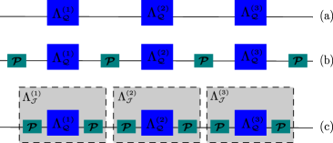
Figure 1: Conversion of the three-time step quantum process $\Lambda_{\mathcal{Q}}$ consisting of the CPTP maps $\Lambda_{\mathcal{Q}}(n)$ shown in line (a) into a classical process by complete measurements, denoted by $\mathcal{P}$. The result is depicted in line (b). In line (c) the intermediate measurements are duplicated, which results in the classical maps $\Lambda_{\mathcal{J}}(n)=\mathcal{P}\circ\Lambda_{\mathcal{Q}}(n)\circ\mathcal{P}$.

As illustrated in Fig. 1, starting from a general quantum process $\Lambda_{\mathcal{Q}}$, we include the complete measurements $\mathcal{P}$ before or after each individual quantum map $\Lambda_{\mathcal{Q}}(n)$. The measurements between two quantum maps can be duplicated without changing the dynamics, which results in the classical maps $\Lambda_{\mathcal{J}}(n)=\mathcal{P}\circ\Lambda_{\mathcal{Q}}(n)\circ\mathcal{P}$.

To find candidate quantum processes $\Lambda_{\mathcal{Q}}$ which may then be checked if they really are valid quantum extensions of a given classical process $\Lambda_{\mathcal{J}}$, we use the following guiding principles: (i) We try to find quantum extensions for each stochastic map $\Lambda_{\mathcal{J}}(n)$, individually. (ii) Both, the classical and the quantum map can be uniquely defined by their action on the basis states $\{|j\rangle\}$. Here, the classical map is determined by the probabilities to jump from the state $|j\rangle$ to any other state. (iii) For the corresponding quantum map, we try to replace as far as possible random “which path” decisions by a superposition of all available options. This is done in such a way that the absolute value square of the transition amplitudes agree with the corresponding classical transition probabilities. (iv) This must be done in such a way that Eq. (4) is fulfilled. As explained in App. A this is not always possible with a single unitary operation. Therefore we also consider conditional unitary operations, where the choice of the operation is conditioned on the outcome of a projective measurement. (v) Once we found a valid quantum extension $\Lambda_{\mathcal{Q}}(n)$, we may define a whole one parameter family of interpolating extensions by the convex sum

$$(1-p)\,\Lambda_{\mathcal{Q}}(n)+p\,\Lambda_{\mathcal{J}}(n)$$ (5)

for $0\leq p\leq 1$. Inserting Eq. (4) into Eq. (5) shows that we can implement this map by simply performing complete measurements $\mathcal{P}$ with probability $p$ after each elementary time step. Then for $p=0$ the system will be maximally coherent while for $p=1$ the process will be completely incoherent classical process.

III Choice of the stochastic process and it’s quantum extension

To test our procedure for constructing quantum extensions of a given classical stochastic process, we consider the zero temperature quenching dynamics of the one-dimensional nearest neighbor Ising model (without magnetic field) [27] with periodic boundary conditions.

III.1 Classical relaxation process

The classical relaxation process starts from a totally disordered initial configuration, corresponding to a very high temperature, where the spins are either up or down at random. We are interested in the relaxation process from this random initial configuration to one of the two ground states, where all spins are aligned to each other, pointing either up or down.

The relaxation process under zero temperature Glauber dynamics [23] is as follows: (i) choose a spin at random; (ii) calculate the energy change ($\Delta E$) of the system if the spin is flipped; (iii) If $\Delta E<0$ flip the spin, if $\Delta E>0$ do nothing, if $\Delta E=0$, choose one of the two options at random with equal probabilities. The process consisting of the steps (i),(ii),(iii) amounts to one elementary (local) operation. For a spin chain of length $N$, one Monte-Carlo step consists of $N$ such elementary operations.

This process is a Markov chain [4], exactly of the type considered in Sec. II.1. If we denote the local operation, which is applied to spin $q$ in the chain by $\mathcal{J}^{(q)}$, then we find for a complete elementary operation:

$$\bm{p}(n+1)=\mathcal{J}\,\bm{p}(n)\;,\qquad\mathcal{J}=\frac{1}{N}\sum_{q=1}^{N}\mathcal{J}^{(q)}\;.$$ (6)

Here, the uniform average taken over all local transition matrices $\mathcal{J}^{(q)}$, implements the random choice of spin $q$ in step (i), of the above list.

Finally, we will write down the transition matrix $\mathcal{J}^{(q)}$ in the basis of all possible classical configurations. For that it is enough to consider the spin $q$ and its immediate neighbors. Let us denote the spin-up state by $|0\rangle$ and the spin-down state by $|1\rangle$, and let us order the configurations of three consecutive spins as $(\,|000\rangle\,,\;|001\rangle\,,\;|010\rangle\,,\;|011\rangle\,,\;|100\rangle\,,\;|101\rangle\,,\;|110\rangle\,,\;|111\rangle\,)$. Then the transition matrix reads

$$\mathcal{J}^{(q)}=\begin{pmatrix}1&0&1&0&0&0&0&0\\ 0&1/2&0&1/2&0&0&0&0\\ 0&0&0&0&0&0&0&0\\ 0&1/2&0&1/2&0&0&0&0\\ 0&0&0&0&1/2&0&1/2&0\\ 0&0&0&0&0&0&0&0\\ 0&0&0&0&1/2&0&1/2&0\\ 0&0&0&0&0&1&0&1\end{pmatrix}\;.$$ (7)

In agreement with the Glauber process, outlined above, the transition matrix leaves the configurations $|000\rangle$ and $|111\rangle$ untouched, it flips the middle spin of the configurations $|010\rangle$ and $|101\rangle$, while flipping the middle spin with probability one half in all other cases.

III.2 Corresponding quantum extensions

In order to find quantum extensions of the process described in Sec. III.1, it is enough to find a quantum extensions $\Lambda_{\mathcal{Q}}$ of the classical transition matrix $\mathcal{J}$. Just as in the classical case, we will implement $\Lambda_{\mathcal{Q}}$ as a uniform mixture of local operations $\Lambda_{\mathcal{Q}}^{(q)}$, which are applied to spin $q$ and its immediate neighbors. Therefore,

$$\Lambda_{\mathcal{Q}}=\frac{1}{N}\sum_{q=1}^{N}\Lambda_{\mathcal{Q}}^{(q)}\;.$$ (8)

In this way, the problem is reduced to finding quantum extensions $\Lambda_{\mathcal{Q}}^{(q)}$ for the three-spin classical operation $\mathcal{J}^{(q)}$.

As explained in detail in App. A, a single unitary operation cannot be a valid quantum extension of the map $\mathcal{J}^{(q)}$ given in Eq. (7). One needs at least two Kraus operators, which may be chosen as conditional unitary operations. Dividing the three-spin Hilbert space into two subspaces, defined by the projectors, $\hat{P}=|010\rangle\langle 010|+|101\rangle\langle 101|$ and its complement $\hat{P}_{\rm c}$, we may write for the desired quantum operation

$$\Lambda_{\mathcal{Q}}^{(q)}[\varrho]=\hat{\sigma}_{x}\,\hat{P}\,\varrho\,\hat{P}\,\hat{\sigma}_{x}+\hat{U}_{X}\,\hat{P}_{\rm c}\,\varrho\,\hat{P}_{\rm c}\,\hat{U}_{X}^{\dagger}\;.$$ (9)

Here, the Pauli matrix $\hat{\sigma}_{x}$ is applied to central spin, whereas the unitary matrix $\hat{U}_{X}$ can be decomposed into the orthogonal sum

$$\hat{U}_{X}=\mathds{1}_{\{|000\rangle,|111\rangle\}}\oplus X_{\{|001\rangle,|011\rangle\}}\oplus X_{\{|100\rangle,|110\rangle\}}\;,$$ (10)

where $X$ may be any $2$$\times$$2$ dimensional unitary matrix with matrix elements of the same magnitude, $1/\sqrt{2}$. Again, in App. A we explain how one arrives at this result and we show that $\Lambda_{\mathcal{Q}}^{(q)}$ is indeed a valid quantum extension, which fulfills Eq. (4).

In the numerical simulations to be presented below, we will focus on two different choices for $X$, namely

$$H=\frac{1}{\sqrt{2}}\begin{pmatrix}1&1\\ 1&-1\end{pmatrix}\;,\qquad S=\frac{1}{\sqrt{2}}\begin{pmatrix}1&-1\\ 1&1\end{pmatrix}\;.$$ (11)

Here, $H$ is the Hadamard gate and $S$ is a SU$(2)$ matrix. As we will see, the two options lead to the resulting quantum processes with very different behaviors.

III.3 Observables

In this section, we introduce the observables we are going to analyze. For studying the relaxation process in time, we measure time in units of Monte-Carlo time steps (MCS), such that $t$ increases by one unit, whenever $N$ elementary operations $\Lambda_{\mathcal{Q}}$ are completed.

Average number of domain walls.

For a classical Ising spin chain, starting from a disordered state, the average number of domain walls $D_{w}(t)$ decays as $t^{-1/z}$ indicating that the average domain size increases as $t^{1/z}$, where $z$ is domain growth exponent [28].

If $n_{D}(j)$ is the number of domain walls of the spin configuration $|j\rangle$ ($0\leq j\leq 2^{N}-1$), we define the corresponding quantum observable $\hat{D}_{\rm W}=\sum_{j}n_{\rm D}(j)\,|j\rangle\langle j|$. Hence the expectation value for an evolving mixed quantum state $\varrho(t)$ is $\langle\hat{D}_{\rm W}\rangle(t)={\rm tr}\big{[}\hat{D}_{\rm W}\,\varrho(t)\big{]}$.

Relaxation time

The dynamics of the classical process always ends in a state, where all spins point in the same direction, either up, $|\bm{0}\rangle=|00\cdots 0\rangle$, or down, $|\bm{1}\rangle=|11\cdots 1\rangle$. The quantum process, however, can also end in a superposition of the two states. Thus, the probability to find the system after time $t$ at equilibrium, is $P_{\rm Eq}(t)={\rm tr}\big{[}\hat{P}_{\rm Eq}\,\varrho(t)\big{]}$, where $\hat{P}_{\rm Eq}=|\bm{0}\rangle\langle\bm{0}|+|\bm{1}\rangle\langle\bm{1}|$. In the simulations below, we report the half life $t_{1/2}$ in MCS, which is such that $P_{\rm Eq}(t_{1/2})=1/2$ (see App. C for further elaboration).

Coherence

Quantum extensions differ crucially from their classical ancestor due to the presence of superpositions. These are quantified conveniently with the help of the coherence measure

$$C(t)=\sum_{i\neq j}|\varrho_{ij}(t)|\;,$$ (12)

as introduced in [18].

IV Numerical simulations

We simulated different quantum extensions of the classical relaxation process for the zero temperature quench of an Ising spin chain. At their core there are the unitary matrices $H$ and $S$ [Eq. (11)], which generate the required quantum superpositions. We label the resulting processes by “HAD” and “SYH”, respectively. As explained above, once a quantum extension $\Lambda_{\mathcal{Q}}$ is found, we can construct convex combinations of that process with the original classical process as described in Eq.(5).This allows us to control the degree of coherence introduced in the system.

In practice this means that after each elemental quantum map $\Lambda_{\mathcal{Q}}^{(q)}$, we apply a complete measurement $\mathcal{P}$ with probability $p$. We consider three cases: $p=0$ (maximally coherent without complete measurements), $p=1/N$ (on average one complete measurement per MCS), $p=1$ (complete measurements with certainty reproducing the classical process). In that latter case, the two options “HAD” and “SYH” yield exactly the same dynamics. This leaves us with five different processes listed in Tab. (1).

Table 1: Interpolation of the quantum extensions by means of the parameter $p$, as described in Eq. (5). The first row list the different processes considered here. The second row shows the value of $p$, which depends of the average number of projective measurements. The last row specifies the number of these projective measurements per MC step for each of the defined processes.

case:	HAD-0	HAD-1	Class	SYH-1	SYH-0
$p$	0	$1/N$	1	$1/N$	0
measure. rate	0	1	$N$	1	0

Methodology

In all cases, we consider an even number of spins $N$, with random initial configurations, where there are exactly as many spins pointing upward as downward. To avoid the evolution of huge density matrices, we use an unraveling method [16, 29]. That is, we compute the evolution of a large number of pure states, $\{\Psi_{\alpha}(n)\}_{1\leq\alpha\leq N_{\rm sam}}$, and approximate the density matrix at multiples of the MCS as

$$\varrho(t)\approx\frac{1}{N_{\rm sam}}\sum_{\alpha}|\Psi_{\alpha}(Nt)\rangle\langle\Psi_{\alpha}(Nt)|\;,$$ (13)

where $t$ is time in MCS. In the present case, the unraveling is easy to realize, since the whole process has been decomposed into random choices, measurements and conditional unitary operations [see App. B for details]. Using a sparse matrix storage format for the density matrices, We have been able to perform simulations up to $N=20$ spins averaging over $N_{\rm sam}=24\,000$ random initial configurations [30].

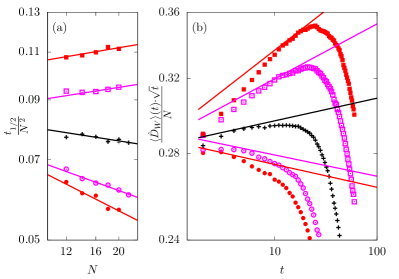
Figure 2: Panel (a): half life $t_{1/2}$ (in units of MCS) divided by $N^{2}$ vs. $N$ (the length of the spin chain) in a log-log plot. Points are numerical simulations, the straight lines best fits. Panel (b): Average number of domain walls $\langle\hat{D}_{\rm W}\rangle$ multiplied by $\sqrt{t}/N$ vs. $t$ for the different process types for $N=20$. In both panels the symbols correspond to: HAD-0 (), HAD-1(), Class($+$), SYH-1 (), and SYH-0 ().

On panel (a), Fig. (2) shows the half-time $t_{1/2}$ of the relaxation process as a function of the number of spins $N$. In the plot, we divide $t_{1/2}$ by $N^{2}$ which corresponds to the scaling of the relaxation time for the classical process as $N\to\infty$ [28]. We show the results for the five different processes, described in Tab. 1. The finite negative slope in the classical case, seems to indicate that $t_{1/2}\sim N^{z}$ with $z<2$. We checked that this is due to the small system size. For $N\gtrsim 80$ one recovers the expected value $z\approx 2$. The quantum extensions show very different scaling exponents. For the HAD cases the exponents are larger, for the SYH cases smaller than in the classical case. These findings are remarkable, in view of the fact that the coherence which is built up during the process is transient and from a global perspective relatively week. The apparent acceleration of the relaxation process is also remarkable; in particular as it seems to persist in the large $N$ limit.

On panel (b), the figure shows the decay of the average number of domain walls with time for the largest spin chain ($N=20$). Here, $\langle\hat{D}_{\rm W}\rangle$ is multiplied by $\sqrt{t}/N$ which would compensate the expected classical, large-$N$, power-law decay. In that way, data which are showing that power-law decay with $z=2$ would lie on a horizontal line. On general grounds the scaling coefficients for the half times in panel (a) are related to the scaling coefficients for the decay of $\langle\hat{D}_{\rm W}\rangle$ as $t_{1/2}\sim N^{z}$ and $\langle\hat{D}_{\rm W}\rangle\sim t^{-1/z}$ [28]. Thus, the solid lines in panel (b) show the power-laws obtained from the exponents estimated in panel (a).

For a realistic macroscopic relaxation process, the natural unit of time is the time it takes for a macroscopic number of constituents to change their state. In our simulations, this time scale is the MCS. So one could expect that if one removes all coherences at every MCS, that the macroscopic observables should behave essentially as in the classical process. Our results for the cases HAD-1 and SYH-1 show that this is not the case. Both, the half times plotted in panel (a) and the average number of domain walls plotted in panel (b) are closer to the maximally quantum cases (without the complete projective measurements) than to the classical case. This quite proves that provided the generation of coherence is sufficiently effective even extremely short decoherence times will not be sufficient to suppress the particular properties of the quantum process.

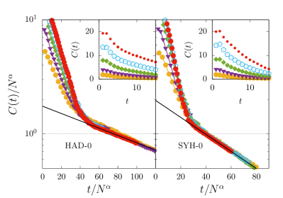
Figure 3: Coherence measure from Eq. (12) as a function of time for different chain lengths, $N=12\,(\leavevmode\hbox to5.69pt{\vbox to5.69pt{\text{[drawing]}}})$; 14 $(\leavevmode\hbox to5.69pt{\vbox to5.69pt{\text{[drawing]}}})$; 16 $(\leavevmode\hbox to6.04pt{\vbox to6.04pt{\text{[drawing]}}})$; 18 $(\leavevmode\hbox to6.67pt{\vbox to6.67pt{\text{[drawing]}}})$; 20 $(\leavevmode\hbox to5.69pt{\vbox to5.69pt{\text{[drawing]}}})$. The inset shows the original data, for short times. The main plot shows the data collapse at large times following the scaling law given in Eq. (14).

Figure 3 shows the coherence measure from Eq. (12) as a function of time, for different chain lengths. Initially there is a steep increase with a pronounced maximum after a few MCS, followed by an apparently exponential decay. The maximum value of $C(t)$ increases with $N$, but slower than exponential. Since the number of non-diagonal elements of $\varrho(t)$ is $O(2^{N})$, this indicates that the overall amount of coherence is rather small. However as we have shown in figure 2, the amount of coherence is enough to change the behavior of the other observables significantly. The scaled semi-log plot in the main figure, shows that the coherence decays exponentially for all times, with different decay rates at short and large times. For large $t$, a scaling form can be written as

$$C(t)\sim N^{\alpha}\,\exp(k\,t/N^{\alpha}),$$ (14)

where $\alpha=1.91\pm 0.014$, $k\simeq 0.017$ for SYH-0, and $\alpha=2.16\pm 0.02$, $k\simeq 0.007$ for HAD-0. The scaling form of $C(t)$ is more complex for short times [31].

One could have assumed that coherence in general might speed up the relaxation process for similar reasons than in the case of the Grover quantum search algorithm [32]. Instead of applying the energy-minimizing spin-flip operations to individual configurations sequentially, coherence allows to apply these operations in parallel to several configurations. Our results show that the situation is more complicated. Almost the same amount of coherence (at the early stage of the process) can either lead to a speed-up or a slowing down of the relaxation process, depending on nothing else but the unitary spin operations employed (HAD or SYH). Interestingly, in the HAD case, the system not only takes a much longer time to reach the equilibrium subspace, it also conserves coherence for a much longer time. Hence, one can say that it is the conservation of coherence which makes it more difficult for the system to find its way to the equilibrium subspace. Of course it would be very desirable and in principle it should be possible to discover the mechanism behind such different behaviors. This requires more detailed studies of the relaxation process itself, which will be left as a task for the future.

V Conclusions and Discussion

Through a new concept that we called quantum extension, we find quantum processes associated with a given Markovian classical stochastic process. In physical terms, this association means that sufficiently frequent observations of the quantum process will convert those processes into the original classical one. This construction does not need an auxiliary system [24, 25]. In other words, unlike in the case of quantum walks [33], our construction does not extend the state space of the original classical process [7].

We apply this new approach to the Glauber relaxation process of a linear Ising chain under a quench to zero temperature. We characterize the coherence of the system in different temporary regimes. Finally, we analyze the process to reach the equilibrium subspace, providing strong evidence that the relaxation times scale differently, for different quantum extensions. Among those, we find at least one process which is faster than the classical case. For a long time stochastic dynamics has been studied for several systems classically including the spin systems for which the real world is quantum. Our construction of “quantum extensions” is useful for studying the dynamics of such systems in a more realistic way.

Our findings may be particularly relevant in areas such as quantum biology and quantum computation. There are increasing experimental evidences [34, 35, 36] for the presence of coherence in biological processes. Currently the main question is to what extent this coherence is necessary for the functioning and efficiency of these processes. In this context, our results (in particular those for HAD-1 and SYH-1) show that even very short coherence times can be compensated by the continuous generation of superpositions, in such a way that the relaxation of macroscopic observables is strongly changed. The application of our approach to such biological processes, may therefore shed new light on these questions.

In the field of quantum computations, quantum annealers [37, 38] are designed to find the energetic minima of Ising-type Hamiltonians. However the general purpose of quantum computers are to implement idealistic unitary algorithms with the help of quantum error correction at the expense of an enormous number of additional qubits [39, 40]. In this area, our approach could pave the way to form quantum operations which are partially incoherent, but still conserve/generate sufficient coherence to outperform a classical algorithm.

VI acknowledgements

The authors acknowledge the use of Leo-Atrox supercomputer at the CADS supercomputing center. This work has been financially supported by the Conacyt project “Ciencias de Frontera 2019”, number 10872.

Appendix A Quantum stochastic map

In order to find quantum extensions $\Lambda_{\mathcal{Q}}$ of a classical stochastic operation $\mathcal{J}$, we use the Kraus operator representation [41]. In that case, $\Lambda_{\mathcal{Q}}$ is defined in terms of a set of Kraus operators as

$$\Lambda_{\mathcal{Q}}\quad:\quad\varrho\to\varrho^{\prime}=\sum_{r}\hat{\mathcal{K}}_{r}\,\varrho\,\hat{\mathcal{K}}_{r}^{\dagger}\;,\quad\sum_{r}\hat{\mathcal{K}}_{r}^{\dagger}\hat{\mathcal{K}}_{r}=\mathds{1}\;.$$ (15)

It is a very difficult task to systematically analyze all possible quantum extensions in terms of such general Kraus operators. We therefore consider a more restrictive set of quantum operations, namely conditional unitary operations. In physical terms, that amounts to a projective measurement, with subsequent unitary operations which are conditioned on the measurement outcomes. In other words, for an observable $\hat{A}$ with the spectral decomposition

$$\hat{A}=\sum_{r}a_{r}\;\hat{P}_{r}\;,\quad\hat{P}_{r}\,\hat{P}_{s}=\delta_{rs}\,\hat{P}_{r}\;,\quad\sum_{r}\hat{P}_{r}=\mathds{1}\;,$$ (16)

and arbitrary unitary operators $U_{r}$, we choose the Kraus operators as

$$\hat{\mathcal{K}}_{r}=\hat{U}_{r}\,\hat{P}_{r}\,\;.$$ (17)

A case of particular interest is the case of a completely unitary operation, when $\Lambda_{\mathcal{Q}}$ contains only one element, $\hat{\mathcal{K}}_{1}=\hat{U}$ ($\hat{P}_{1}=\mathds{1}$). In this case the condition for a valid quantum extension, Eq. (4), requires that $\Lambda_{\mathcal{J}}=\mathcal{P}\circ\Lambda_{\mathcal{Q}}\circ\mathcal{P}$. For an arbitrary density matrix $\varrho$ and $\varrho^{\prime}=U\,\varrho\,U^{\dagger}$, this is equivalent to the condition that

$$\Lambda_{\mathcal{J}}:\quad\varrho^{\prime}_{jj} =\sum_{k}\mathcal{J}_{jk}\varrho_{kk}$$ (18)

$$\,.\mathcal{P}\circ\Lambda_{\mathcal{Q}}\circ\mathcal{P}:\quad\varrho^{\prime}_{jj} =\sum_{k}\langle j|\,\hat{U}\,|k\rangle\langle k|\,\varrho\,|k\rangle\langle k|\,\hat{U}^{\dagger}\,|j\rangle$$

$$=\sum_{k}|U_{jk}|^{2}\,\varrho_{kk}\,,$$ (19)

and when equations (18) and (A) are compared, the following condition is obtained

$$\forall\,j,k:\qquad\mathcal{J}_{jk}=|U_{jk}|^{2}\,.$$ (20)

For our particular example of the classical map defined in Eq.(7), such a unitary operation cannot exist. This is because the required unitary matrix must have matrix elements $U_{11}$ and $U_{13}$ of magnitude equal to one, so that the corresponding columns cannot be orthogonal.

If a single unitary operation does not work, we can try to find a quantum operations with two Kraus operators. As explained above, we search for Kraus operators which describe a conditional unitary operation. That means, depending on whether the system is found in one subspace $\hat{P}$ or not (subspace $\hat{P}^{\rm c}$) we apply one unitary operation $\hat{U}$ or another, $\hat{V}$. To simplify the task even more, we assume that the basis states are eigenstates of $\hat{P}$ and $\hat{P}^{\rm c}$. With this, the requirement for a valid operator sum representation is fulfilled:

$$\hat{\mathcal{K}}_{1}=\hat{U}\,\hat{P}\;,\quad\hat{\mathcal{K}}_{2}=\hat{V}\,\hat{P}^{\rm c}$$

$$\textrm{with}\quad\hat{\mathcal{K}}_{1}^{\dagger}\hat{\mathcal{K}}_{1}+\hat{\mathcal{K}}_{2}^{\dagger}\hat{\mathcal{K}}_{2}=\hat{P}+\hat{P}^{\rm c}=\mathds{1}\,.$$ (21)

Now, from the right-hand side of equation (4), the following diagonal elements of $\varrho^{\prime}$ are obtained

$${\varrho}_{jj}^{\prime} =U_{jk}\,\hat{P}_{kk}\,\varrho_{kk}\,\hat{P}_{kk}\,U_{jk}^{*}+V_{jk}\,\hat{P}^{\rm c}_{kk}\,\varrho_{kk}\,\hat{P}^{\rm c}_{kk}\,V_{jk}^{*}$$ (22)

and the requirement for a valid quantum extension now reads:

$$\forall j,k:\quad J_{jk}=\begin{cases}|U_{jk}|^{2}&:\hat{P}\,|k\rangle=|k\rangle\\ |V_{jk}|^{2}&:\hat{P}\,|k\rangle=0\end{cases}\;.$$ (23)

Now let us return to our particular case. A quantum extension associated to the classical map Eq. (7) that satisfies condition (23) is defined in Eq. (9) where the unitary operations $U$ and $V$ are chosen as $\hat{U}=\hat{\sigma}_{x}^{(q)}$, $\hat{V}=\hat{U}_{X}$ (defined in Eq. 10), which in matrix form look like

$$\mathcal{K}_{1} =\sigma_{x}^{(q)}\,P=\begin{pmatrix}0&0&1&0&0&0&0&0\\ 0&1&0&0&0&0&0&0\\ 1&0&0&0&0&0&0&0\\ 0&0&0&1&0&0&0&0\\ 0&0&0&0&1&0&0&0\\ 0&0&0&0&0&0&0&1\\ 0&0&0&0&0&0&1&0\\ 0&0&0&0&0&1&0&0\end{pmatrix}\begin{pmatrix}0&0&0&0&0&0&0&0\\ 0&0&0&0&0&0&0&0\\ 0&0&1&0&0&0&0&0\\ 0&0&0&0&0&0&0&0\\ 0&0&0&0&0&0&0&0\\ 0&0&0&0&0&1&0&0\\ 0&0&0&0&0&0&0&0\\ 0&0&0&0&0&0&0&0\end{pmatrix}\;,$$ (24)

$$\mathcal{K}_{2} =U_{X}\,P^{\rm c}=\begin{pmatrix}1&0&0&0&0&0&0&0\\ 0&X_{11}&0&X_{12}&0&0&0&0\\ 0&0&1&0&0&0&0&0\\ 0&X_{21}&0&X_{22}&0&0&0&0\\ 0&0&0&0&X_{11}&0&X_{12}&0\\ 0&0&0&0&0&1&0&0\\ 0&0&0&0&X_{21}&0&X_{22}&0\\ 0&0&0&0&0&0&0&1\end{pmatrix}\begin{pmatrix}1&0&0&0&0&0&0&0\\ 0&1&0&0&0&0&0&0\\ 0&0&0&0&0&0&0&0\\ 0&0&0&1&0&0&0&0\\ 0&0&0&0&1&0&0&0\\ 0&0&0&0&0&0&0&0\\ 0&0&0&0&0&0&1&0\\ 0&0&0&0&0&0&0&1\end{pmatrix}\;,$$ (25)

We can see that this choice fulfills Eq.(3), where $\hat{\mathcal{K}}_{1}$ takes care of column 3 and 6 while $\hat{\mathcal{K}}_{2}$ takes care of all the other columns. Of course,

$$X=\begin{pmatrix}X_{11}&X_{12}\\ X_{21}&X_{22}\end{pmatrix}$$ (26)

must be a unitary matrix where all matrix elements have absolute value squared equal to one half. For that we use the matrices defined in Eq. (11).

Appendix B Numerical simulation: Unraveling

In this section we describe a simplified version of the unraveling method presented in [16]. This method is easy to implement and with proper optimization reduces the computational costs of processing and memory. The method consists of the following:

• An initial state $|\Psi_{\alpha}(0)\rangle$ is taken from the set of basis states with zero magnetization, i.e., half of spins up and half down.

• A spin is chosen randomly from the chain to which the local operation (LO) is applied. The LO consists of an element of the set of Kraus operators $\{\hat{\mathcal{K}}_{r}\}$. Then, with a probability $q_{r}=\langle\Psi_{\alpha}(0)|\hat{\mathcal{K}}_{r}^{\dagger}\hat{\mathcal{K}}_{r}|\Psi_{\alpha}(0)\rangle$ the LO $\hat{\mathcal{K}}_{r}$ transform the initial state $|\Psi_{\alpha}(0)\rangle$ as follows

  $$|\Psi_{\alpha}(0)\rangle\,\mapsto\,|\Psi_{\alpha}(1)\rangle=\frac{\hat{\mathcal{K}}_{r}|\Psi_{\alpha}(0)\rangle}{\sqrt{q_{r}}}\,.$$

• With probability $p$ it is decided to apply a complete projective measurement. This measurement collapses the state $|\Psi_{\alpha}(1)\rangle$ to one of the elements of the basis, which eliminates any trace of coherences created in the previous step.

At each discrete time $n=1,2,\ldots$, steps II-III are repeated. The state of the system is saved at each Monte-Carlo (MC) time $t$, i.e., $t=N\cdot n$. The evolution ends at some time $t^{*}$ when the system reach the equilibrium subspace. Which is equivalent to $|\Psi_{\alpha}(t^{*})\rangle=c_{0}(t^{*})|\bm{0}\rangle+c_{1}(t^{*})|\bm{1}\rangle$ ($|\bm{0}\rangle=|00\cdots 0\rangle$ and $|\bm{1}\rangle=|11\cdots 1\rangle$) with $|c_{0}(t^{*})|^{2}+|c_{1}(t^{*})|^{2}=1$. This protocol is repeated for each of the initial states $\{|\Psi_{\alpha}(0)\rangle\}_{\alpha=1,\ldots,N_{\textrm{sam}}}$, so that the density matrix at each MC time is approximated as follows

$$\varrho(t) \approx\frac{1}{N_{\textrm{sam}}}\sum_{\alpha}|\Psi_{\alpha}(t)\rangle\langle\Psi_{\alpha}(t)|\,$$

Appendix C Estimation of the relaxation time

For the classical evolution, we say that the system has been reached the equilibrium state when it is found in an ordered phase, in other words, all the spins are up or all down. Meanwhile, for the quantum evolution, it is necessary to consider the equilibrium when the system is found in a superposition of the two possible states $|\bm{0}\rangle=|00\cdots 0\rangle$ and $|\bm{1}\rangle=|11\cdots 1\rangle$.

$$|\Psi_{\alpha}(t)\rangle=c_{0}(t)|\bm{0}\rangle+c_{1}(t)|\bm{1}\rangle$$

$$where\quad(|c_{0}(t)|^{2}+|c_{1}(t)|^{2}=1)\,.$$ (27)

The total number of elements in the ensemble can be written as $N_{{\rm sam}}=N_{1}+N_{2}+\cdots+N_{t_{\rm max}}$, where $N_{t}$ corresponds to the number of elements of the ensemble that reach the equilibrium subspace at MC time step $t$. So, we define the probability that the system reach the equilibrium subspace at time $t$ as

$$P_{t}=\frac{N_{t}}{N_{{\rm sam}}}$$

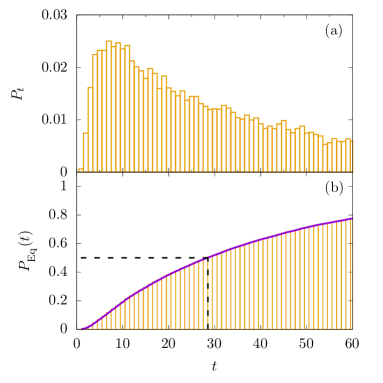
Figure 4: Panel a: Occurrence probability $P_{t}$ for a 16-spin chain and ”SYH” process. Panel b: Cumulative probability distribution calculated by the approximation of the integral (orange boxes). Alternatively, calculated by means of $\mbox{tr}[\hat{P}_{{}_{\rm Eq}}\varrho(t)]$ ( solid violet line). The dashed straight line indicates the value of $t_{1/2}$ obtained when $\hat{P}_{{}_{\rm Eq}}=1/2$.

This probability of occurrence is plotted in figure 4 (panel-a) for a chain with 16-spin.

Similarly we define the half-life $t_{{}_{1/2}}$, the way it is defined in radioactive decay processes [42], as the time required for half of the elements of the ensemble to reach the equilibrium subspace. To estimate the half-life as a function of the length of the spin chain (figure 2-b in the main text), we first calculate the cumulative probability distribution

$$P_{{\rm Eq}}(t)=\int_{0}^{t}P_{t^{\prime}}\,dt^{\prime}$$ (28)

and calculate the time for which $P_{{\rm Eq}}=1/2$, as shown in figure 4 (panel-b, black dashed line).

Alternatively, we can define an observable $\hat{\mathcal{O}}=\lambda_{1}\hat{P}_{{}_{\rm Eq}}+\lambda_{2}\hat{P}^{c}_{{}_{\rm Eq}}$ where $\hat{P}_{{}_{\rm Eq}}$ projects to the equilibrium subspace and $\hat{P}^{c}_{{}_{\rm Eq}}=\mathds{1}-\hat{P}_{{}_{\rm Eq}}$. Then, the probability of reaching the equilibrium subspace $P_{{\rm Eq}}(t)$ is given by

$$P_{{\rm Eq}}(t)=\mbox{tr}[\hat{P}_{{}_{\rm Eq}}\,\varrho(t)]$$ (29)

see figure 4 (lower panel, solid violet line).

References

- [1] S. Karlin and H. M. Taylor, First Course in Stochastic Processes (Academic Press, San Diego, 1975).
- [2] V. Privman (Ed.), Nonequilibrium Statistical Mechanics in One Dimension (Cambridge University Press, Cambridge, 1997).
- [3] W. Paul and J. Baschnagel, Stochastic Processes: From Physics to Finance (Springer International Publishing, Switzerland, 2013).
- [4] N. G. van Kampen, Stochastic Processes in Physics and Chemistry (North Holland, Amsterdam, 2007).
- [5] P. C. Bressloff, Stochastic Processes in Cell Biology (Springer International Publishing, Switzerland, 2014).
- [6] M. Baron, Probability and Statistics for Computer Scientists, 2nd Edition (CRC Press, Boca Raton, 2015).
- [7] S. Chandrasekhar, Stochastic Problems in Physics and Astronomy, Rev. Mod. Phys. 15, 1 (1943).
- [8] V. Zaburdaev, S. Denisov, and J. Klafter, Lévy walks, Rev. Mod. Phys. 87, 483 (2015).
- [9] G. E. Uhlenbeck and L. S. Ornstein, On the Theory of the Brownian Motion, Phys. Rev. 36, 823 (1930).
- [10] R. J. Adler, The Geometry of Random Fields (SIAM, Philadelphia, 2010).
- [11] K. B. Athreya and P. E. Ney, Branching Process (Springer, Berlin, 1972).
- Sudarshan et al. [1961] E. C. G. Sudarshan, P. M. Mathews, and J. Rau, Stochastic dynamics of quantum-mechanical systems, Phys. Rev. 121, 920 (1961)
- Gorini et al. [1976] V. Gorini, A. Kossakowski, and E. C. G. Sudarshan, Completely positive dynamical semigroups of n‐level systems, J. Math. Phys. 17, 821 (1976)
- Lindblad [1976] G. Lindblad, On the generators of quantum dynamical semigroups, Commun. Math. Phys. 48, 119 (1976)
- [15] E. B. Davies, Quantum stochastic processes, Commun. Math. Phys. 15, 277 (1969).
- Breuer and Petruccione [2002] H.-P. Breuer and F. Petruccione, The Theory of open quantum systems (Oxford University Press, 2002)
- Giulini et al. [1996] D. Giulini, E. Joos, C. Kiefer, J. Kupsch, I.-O. Stamatescu, and H.-D. Zeh, Decoherence and the appearence of a classical world in quantum theory (Springer, Berlin, 1996)
- Baumgratz et al. [2014] T. Baumgratz, M. Cramer, and M. B. Plenio, Quantifying coherence, Phys. Rev. Lett. 113, 140401 (2014)
- Winter and Yang [2016] A. Winter and D. Yang, Operational resource theory of coherence, Phys. Rev. Lett. 116, 120404 (2016)
- Chitambar and Gour [2016] E. Chitambar and G. Gour, Critical examination of incoherent operations and a physically consistent resource theory of quantum coherence, Phys. Rev. Lett. 117, 030401 (2016)
- [21] A. Smirne and D. Egloff and M. G. Díaz and M. B. Plenio and S. F. Hulega, Coherence and non-classicality of quantum Markov processes, Quantum Sci. Technol. 4, 01LT01 (2018).
- [22] Chen, H.-B. and Lo, P.-Y. and Gneiting, C. and Bae, J. and Chen, Y.-N. and Nori, F., Quantifying the nonclassicality of pure dephasing, Nat. Comm., 10, 3794 (2019).
- [23] R. J. Glauber, J. Math. Phys 4, 294 (1963)
- [24] I. Bengtsson and K. Życzkowski, Geometry of Quantum States: An Introduction to Quantum Entanglement, (Cambridge University Press, Cambridge, 2006).
- [25] T. Heinosaari and M. Ziman, The mathematical language of quantum theory: From uncertainty to entanglement, (Cambridge University Press, Cambridge, 2011).
- [26] Kok Chuan Tan and Hyunseok Jeong, Phys. Rev. Lett. 121, 220401 (2018)
- [27] E. Ising, Beitrag zur Theorie des Ferromagnetismus, Z. Phys., 31 (1): 253 (1925).
- [28] A. J. Bray, Theory of phase-ordering kinetics, Adv. Phys. 43, 357 (1994).
- [29] K. Mølmer and Y. Castin and J. Dalibard, Monte Carlo wave-function method in quantum optics, J. Opt. Soc. B, 10, 524 (1993); Wave-function approach to dissipative processes in quantum optics, Phys. Rev. Lett, 68, 580 (1992).
- [30] Using a single XEON core with 512GB RAM, it takes 5-6 days to simulate a spin chain of 20 spins for 24000 realisations.
- [31] G. Montes, S. Biswas and T. Gorin, Unpublished
- [32] Grover, Lov K., A Fast Quantum Mechanical Algorithm for Database Search, STOC ’96, Proceedings of the Twenty-Eighth Annual ACM Symposium on Theory of Computing, 212 (1996) (Association for Computing Machinery, New York, NY, USA),
- [33] S. E. Venegas-Andraca, Quantum walks: a comprehensive review, Quantum Information Processing 11, 1015 (2012).
- [34] A. Marais and B. Adams and A. K. Ringsmuth and M. Ferretti and J. M. Gruber and R. Hendrikx and M. Schuld and S. L. Smith and I. Sinayskiy and T. P. J. Krüger and F. Petruccione and R. van Grondelle, The future of quantum biology, Journal of The Royal Society Interface 15, 20180640 (2018).
- [35] Cao et al., Quantum Biology revisited, Sci. Adv. 6, eaaz4888 (2020).
- [36] Y. Kim and F. Bertagna and E. M. D’Souza and D. J. Heyes and L. O. Johannissen E. T. Nery and A. Pantelias and A. Sanchez-Pedreño Jimenez and L. Slocombe and M. G. Spencer and J. Al-Khalili and G. S. Engel and S. Hay and S. M. Hingley-Wilson and K. Jeevaratnam and A. R. Jones and D. R. Kattnig and R. Lewis and M. Sacchi and N. S. Scrutton and S. R. P. Silva and J. McFadden, Quantum Biology: An Update and Perspective, Quantum Reports 3, 80 (2021).
- [37] P. Weinberg and M. Tylutki and J. M. Rönkkö and J. Westerholm and J. A. Åström and P. Manninen and P. Törmä and A. W. Sandvik, Scaling and Diabatic Effects in Quantum Annealing with a D-Wave Device, Phys. Rev. Lett. 124, 090502 (2020).
- [38] M. Jünger and E. Lobe and P. Mutzel and G. Reinelt and F. Rendl and G. Rinaldi and T. Stollenwerk, Quantum Annealing versus Digital Computing: An Experimental Comparison, ACM J. Exp. Algorithmics 26, 1.9 (2021).
- [39] M. Reiher and N. Wiebe and K. M. Svore and D. Wecker and M. Troyer, Elucidating reaction mechanisms on quantum computers, Proceedings of the National Academy of Sciences 114, 7555 (2017).
- [40] R. Chao and B. W. Reichardt, Fault-tolerant quantum computation with few qubits, npj Quantum Information 4, 42 (2018).
- Kraus et al. [1983] K. Kraus, A. Böhm, J. D. Dollard, and W. Wootters, Lecture notes in physics 190 (1983).
- Burton and Kebler [1960] R. E. Burton and R. W. Kebler, American documentation 11, 18 (1960).