From Contraction Theory to Fixed Point Algorithms
on Riemannian and Non-Euclidean Spaces

Abstract

The design of fixed point algorithms is at the heart of monotone operator theory, convex analysis, and of many modern optimization problems arising in machine learning and control. This tutorial reviews recent advances in understanding the relationship between Demidovich conditions, one-sided Lipschitz conditions, and contractivity theorems. We review the standard contraction theory on Euclidean spaces as well as little-known results for Riemannian manifolds. Special emphasis is placed on the setting of non-Euclidean norms and the recently introduced weak pairings for the $\ell_{1}$ and $\ell_{\infty}$ norms. We highlight recent results on explicit and implicit fixed point schemes for non-Euclidean contracting systems.

I Introduction

Motivated by control, optimization, and machine learning applications, this document provides a simplified and incomplete tutorial about the main contraction theorem and resulting fixed point algorithms. The combination of contraction theory and fixed point algorithms originates in the classic ground-breaking paper by Desoer and Haneda [7]; these ideas play a central role in numerical integration of differential equations [8].

The importance of fixed point strategies in modern day data science is described in the recent review [4]. [14] is a recent survey on monotone operators and their application to convex optimization. In this paper, we argue that contraction theory for vector fields is the continuous-time equivalent of these theories. Indeed, strongly monotone operators and gradient vector fields of strongly convex functions are strongly contracting vector fields, modulo a sign change. A central problem in these fields is the design of efficient fixed point algorithms; recent contributions in this spirit are [18, 13].

Of special interest in this paper are contracting systems in non-Euclidean spaces, i.e., vector fields whose flow is a contraction mapping with respect to a non-Euclidean norm. In this context, Aminzare and Sontag were the first to highlight the connections between contraction theory and semi-inner products in [1, 2].

This tutorial is based upon the theory of weak pairings recently developed in [6, 9, 10]. We remark that monotone operators over smooth semi-inner product spaces are studied for example in [15]; here we are precisely interested in nonsmooth polyhedral norms, such as the $\ell_{1}$ and $\ell_{\infty}$ norms. For the same reason (lack of differentiability), contraction theory over Finsler manifolds does not directly apply to the non-Euclidean problems of interest here.

This document also briefly reviews some generalizations to Riemannian manifolds. Contraction theory on Riemannian manifolds originates in the influential work by Lohmiller and Slotine [11]. A formal coordinate-free analysis (with connection to monotone operators) is given in [16]. In the differential geometry literature, the study of geodesically monotonic vector fields initiated in [12] and relevant extensions were obtained in [5, 17].

This document is intended to be a tutorial and makes the following contributions. First, we provide a unified view of the main theorem on contraction and incremental stability in the context of Euclidean, Riemannian and non-Euclidean spaces. Similarly, we present a unified investigation into fixed point algorithms over these three domains. Second, we consider the setting of strongly contracting vector fields with respect to non-Euclidean norms: we analyze and establish convergence factors for the explicit Euler (from [10]), explicit extragradient, and implicit Euler algorithms. Notably, these results provide a starting point for the generalization of convex analysis and monotone operator theory to the setting of strongly contracting vector fields with respect to the norms $\ell_{1}$ and $\ell_{\infty}$. Finally, we include a number of conjectures that will hopefully stimulate further research.

A brief review of matrix measures

We recall the standard $\ell_{p}$ induced norms, $p\in\{1,2,\infty\}$:

$$\|A\|_{2}=\sqrt{\lambda_{\textup{max}}(A^{\top}A)},$$

$$\|A\|_{1}=\max_{j\in\{1,\dots,n\}}\sum_{i=1}^{n}|a_{ij}|,\quad\|A\|_{\infty}=\max_{i\in\{1,\dots,n\}}\sum_{j=1}^{n}|a_{ij}|.$$

where $\lambda_{\textup{max}}(A^{\top}A)$ is the largest eigenvalue of $A^{\top}A$. The matrix measure of $A\in^{n\times n}$ with respect to a norm $\|\cdot\|$ is

$$\mu(A):=\lim_{h\to 0^{+}}\frac{\|I_{n}+hA\|-1}{h}.$$ (1)

From [7] we recall $\mu_{2}(A)=\tfrac{1}{2}\lambda_{\textup{max}}\big{(}A+A^{\top}\big{)}$,

$$\mu_{1}(A)\! =\!\!\max_{j\in\{1,\dots,n\}}\Big{(}a_{jj}+\!\!\!\sum_{i=1,i\neq j}^{n}\!|a_{ij}|\Big{)},\enspace\mu_{\infty}(A)=\mu_{1}(A^{\top}).$$

For $R$ invertible square, we define $\|A\|_{p,R}=\|RA\|_{p}$ and its associated matrix measure $\mu_{p,R}(A)=\mu_{p}(RAR^{-1})$. For $P=P^{\top}\succ 0$, we write $\|x\|_{P}^{2}=\|x\|_{2,P^{1/2}}^{2}=x^{\top}{P}x$. Matrix measures enjoy numerous properties [7]; we present here only the so-called Lumer’s equalities:

$$\mu_{2,P^{1/2}}(A) =\max_{\|x\|_{2,P^{1/2}}=1}x^{\top}PAx$$ (2a)

$$=\min\{b\in\;|\;A^{\top}P+PA\preceq 2bP\}.$$ (2b)

II Contraction and Monotone Operators on the Euclidean Space $(^{n},\ell_{2})$

We start with a very simple motivating discussion. For $b\in$, $f:\rightarrow$ is one-sided Lipschitz (osL) if

$$(x-y)(f(x)-f(y))\leq b(x-y)^{2},\quad \forall x,y$$ (3)

$$\iff\quad f(x)-f(y)\leq b(x-y),\quad \forall x>y$$ (4)

and if $f$ is continuously differentiable

$$\iff\quad f^{\prime}(x)\leq b, \forall x$$ (5)

We refer to (5) as differential one-sided Lipschitz bound (d-osL). We note that

• $f$ is osL with $b=0$ if and only if $f$ weakly decreasing;

• if $f$ is Lipschitz with bound $\ell$, then $f$ is osL with $b=\ell$, whereas the converse is false;

• finally, for the scalar dynamics $\dot{x}=f(x)$, the Grönwall lemma implies $|x(t)-y(t)|\leq\mathop{e}^{bt}|x(0)-y(0)|$.

In what follows, we generalize this simple discussion in numerous directions and study its implications.

II-A Contraction and Incremental Stability

For a continuously differentiable $f:^{n}\rightarrow^{n}$, consider

$$\dot{x}=f(x).$$ (6)

We next state the main theorem of contraction and exponential incremental stability.

Theorem 1 (Equivalences on $(^{n},\ell_{2})$)

For $P=P^{\top}\succ 0$ and $c>0$, the following statements are equivalent:

1. $(f(x)-f(y))^{\top}P(x-y)\leq-c\|x-y\|^{2}_{2,P^{1/2}}$, for all $x,y$;

2. $PD\mkern-2.5mu{f}(x)+D\mkern-2.5mu{f}(x)^{\top}P\preceq-2cP$ for all $x$, or equivalently $\mu_{2,P^{1/2}}(D\mkern-2.5mu{f}(x))\leq-c$ for all $x$;

3. $D^{+}\|x(t)-y(t)\|_{{2,P^{1/2}}}\leq-c\|x(t)-y(t)\|_{{2,P^{1/2}}}$, for all solutions $x(\cdot),y(\cdot)$, where $D^{+}$ is the upper right Dini derivative;

4. $\|x(t)-y(t)\|_{{2,P^{1/2}}}\leq e^{-ct}\|x(0)-y(0)\|_{{2,P^{1/2}}}$, for all solutions $x(\cdot),y(\cdot)$.

A vector field $f$ satisfying any and therefore all of these conditions is said to be $c$-strongly contacting.

We refer to statement (i) as the one-sided Lipschitz condition (osL) and statement (ii) as the differential one-sided Lipschitz (d-osL) (a.k.a. the Demidovich condition). The last two statements are about differential incremental stability (d-IS) and exponential incremental stability (IS), respectively.

Proof:

We include an incomplete sketch of the proof. Statement (i) implies (ii) by letting $y=x+hv$ for some $v\in^{n}$ and taking the limit as $h\to 0^{+}$. Statement (ii) implies (iii) by Coppel’s inequality [7, Lemma A]. Statement (iii) implies (iv) by the Grönwall Comparison Lemma. Statement (iv) implies (i) by a Taylor expansion. ∎

Variations of Theorem 1 hold for (1) forward-invariant convex sets, (2) time-dependent vector fields, and (3) non-differentiable vector fields $f$, where three of the four properties remain equivalent: osL, d-IS, and IS.

For an affine $f(x)=Ax+b$, the osL condition reads

$$(f(x)-f(y))^{\top}P(x-y)=(x-y)^{\top}A^{\top}P(x-y)\\ =(x-y)^{\top}\frac{A^{\top}P+PA}{2}(x-y)\leq-c\|x-y\|_{2,P^{1/2}}^{2}.$$ (7)

Lumer’s equalities (2) imply that the smallest number $-c$ ensuring the osL and d-osL conditions is $-c=\mu_{2,P^{1/2}}(A)$.

II-B Consequences of Contraction: Equilibria

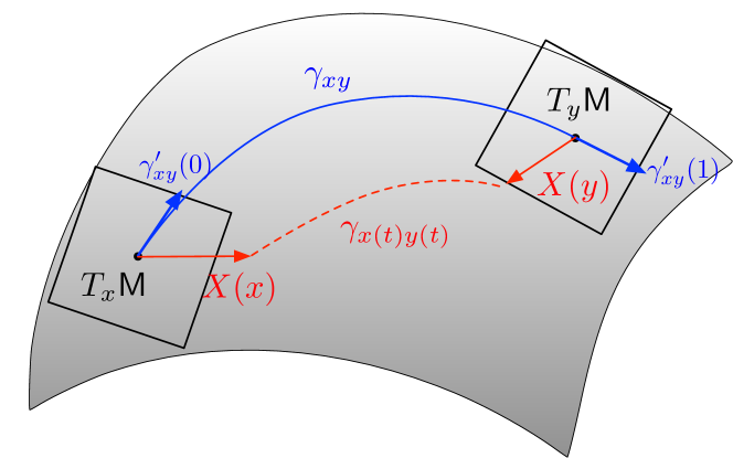
Figure 2: Contractivity of a vector field $X$ on a Riemannian manifold: the length of the geodesic curve $\gamma_{xy}$ connecting any two points $x$ and $y$ decreases along the flow of $X$, as a function of the inner product between $X$ and the geodesic velocity vector at $x$ and $y$.

One of the numerous desirable properties of strongly contracting vector fields is that their flow forgets initial conditions (e.g., see Figure 2) and, in the time-invariant case, globally exponentially converges to a unique equilibrium point. These points are illustrated in the next result.

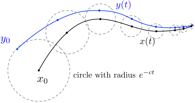
Figure 1: Exponential incremental stability of contracting vector fields. The distance between two trajectories decreases exponentially fast.

Theorem 2 (Equilibria of contracting vector fields)

For a time-invariant vector field $f$ that is $c$-strongly contracting with respect to $\|\cdot\|_{2,P^{1/2}}$, $P=P^{\top}\succ 0$,

1. the flow of $f$ is a contraction, i.e., the distance between solutions exponentially decreases with rate $c$, and

2. there exists a unique equilibrium $x^{*}$ that is globally exponentially stable with global Lyapunov functions

   $$x\mapsto\|x-x^{*}\|_{2,P^{1/2}}^{2}\quad\text{ and }\quad x\mapsto\|f(x)\|_{2,P^{1/2}}^{2}.$$

Proof:

We include an incomplete sketch of the proof. Theorem 5(iv) immediately implies (i) and that, for any positive $\tau$, the flow map of the vector field at time $\tau$ is a contraction map with constant $\mathop{e}^{-c\tau}$. The fixed point of this contraction map is either a period orbit with period $\tau$ (which is impossible) or a fixed point of the flow map. The global Lyapunov functions follow from direct computation. ∎

II-C Equilibrium Computation via Forward Step Method

The study of monotone operators is closely related to the study of contracting vector fields. As it is classic in the study of monotone operators, we here aim to provide an algorithm to compute the equilibrium points of a vector field $f$ (equivalently regarded as an operator):

$$x^{*}\in\operatorname{zero}(f)\quad\iff\quad x^{*}\in\operatorname{fixed}(\mathop{I\mkern-2.5mu{d}}+\alpha f),$$ (8)

for any $\alpha>0$, where $\mathop{I\mkern-2.5mu{d}}$ is the identity map. Here we define $\operatorname{zero}(f)=\{x\in^{n}\;|\;f(x)=0\}$ and $\operatorname{fixed}(\mathop{I\mkern-2.5mu{d}}+\alpha f)=\{x\in^{n}\;|\;x=(\mathop{I\mkern-2.5mu{d}}+\alpha{f})x\}$. A map $f$ is (globally) $\ell$-Lipschitz continuous if

$$\|f(x)-f(y)\|_{2,P^{1/2}}\leq\ell\|x-y\|_{2,P^{1/2}}.$$ (9)

for all $x,y$. We define the operator condition number of a $c$-strongly contracting and $\ell$-Lipschitz continuous map $f$ by

$$\kappa=\ell/c\geq 1.$$ (10)

Remark 3 (Literature comparison)

In the literature on monotone operators, given $P=P^{\top}\succ 0$, the map $g:^{n}\rightarrow^{n}$ is $c$-strongly monotone if

$$(g(x)-g(y))^{\top}P(x-y)\geq c\|x-y\|_{2,P^{1/2}}^{2}.$$ (11)

Clearly, $g$ is $c$-strongly monotone if and only if $-g$ is $c$-strongly contracting.

Next, we compare the operator condition number of a contracting affine $f(x)=Ax+b$, $A\in^{n\times{n}}$, with the standard contraction number of $A$. First, recall that, given a norm $\|\cdot\|$, the condition number of a square invertible matrix $A$ is $\kappa(A)=\|A\|\|A^{-1}\|$. Second, for the $P^{1/2}$-weighted $\ell_{2}$ norm, we know from (7) that the contraction rate of $f$ equals $\mu_{2,P^{1/2}}(A)$. Accordingly, given a norm $\|\cdot\|$, the operator condition number of a square matrix $A$ with $\mu(A)<0$ is

$$\kappa_{\mu}(A)=\frac{\|A\|}{|\mu(A)|}.$$ (12)

From [7], note that $\mu(A)<0$ implies $\|A^{-1}\|\leq 1/|\mu(A)|$. Therefore, $\kappa(A)\leq\kappa_{\mu}(A)$. One can show that the two condition numbers coincide for $A=A^{\top}$ and $P=I_{n}$. $\square$

Given a start point $x_{0}\in^{n}$, the forward step method for the operator $f$, i.e., the explicit Euler integration algorithm for the vector field $f$, is:

$$x_{k+1}=(\mathop{I\mkern-2.5mu{d}}+\alpha f)x_{k}=x_{k}+\alpha f(x_{k}).$$ (13)

Theorem 4

(Optimal step size and contraction factor of forward step method) For $P=P^{\top}\succ 0$, consider a map $f:^{n}\rightarrow^{n}$ with strong contraction rate $c>0$, Lipschitz constant $\ell>0$, and condition number $\kappa=\ell/c$. Then

1. the map $\mathop{I\mkern-2.5mu{d}}+\alpha f$ is a contraction map with respect to $\|\cdot\|_{2,P^{1/2}}$ for

   $$0<\alpha<\frac{2}{c\kappa^{2}},$$

2. the step size minimizing the contraction factor and the minimum contraction factor (that is, the minimal Lipschitz constant of $\mathop{I\mkern-2.5mu{d}}+\alpha f$) are

   $$\alpha_{\textup{E}}^{*} =\frac{1}{c\kappa^{2}},$$ (14)

   $$\ell_{\textup{E}}^{*} =\Big{(}1-\frac{1}{\kappa^{2}}\Big{)}^{1/2}=1-\frac{1}{2\kappa^{2}}+\mathcal{O}\Big{(}\frac{1}{\kappa^{4}}\Big{)}.$$

Proof:

We only sketch the standard proof here:

$$\|(\mathop{I\mkern-2.5mu{d}}+\alpha f)x-(\mathop{I\mkern-2.5mu{d}}+\alpha f)y\|_{2,P^{1/2}}^{2}$$

$$=\|x-y+\alpha(f(x)-f(y))\|_{{2,P^{1/2}}}^{2}$$

$$=\|x-y\|_{{2,P^{1/2}}}^{2}+2\alpha(f(x)-f(y))^{\top}P(x-y)$$

$$\qquad+\alpha^{2}\|f(x)-f(y)\|_{{2,P^{1/2}}}^{2}$$

$$\leq(1-2\alpha c+\alpha^{2}{\ell}^{2})\|x-y\|_{{2,P^{1/2}}}^{2}.$$

It is easy to check that $(1-2\alpha c+\alpha^{2}\ell^{2})<1$ if and only if $0<\alpha<2c/{\ell}^{2}$ and that the minimal contraction factor is $(1-c^{2}/{\ell}^{2})^{1/2}$ at $\alpha^{*}=c/{\ell}^{2}$. ∎

III Contraction Theory and Monotone Operators on Riemannian Manifolds

In this section we consider a Riemannian manifold $(\textsf{M},\mathbb{G})$ with associated Levi-Civita connection $\nabla$, geodesic distance $\mathrm{d}_{\mathbb{G}}$, and parallel transport $P(\gamma)$ along a geodesic arc $\gamma$. Let $\langle\!\langle{\cdot},{\cdot}\rangle\!\rangle_{\mathbb{G}}$ denote the inner product associated to $\mathbb{G}$ and $\gamma^{\prime}$ denote the velocity vector along a geodesic arc.

Loosely speaking, a vector field $X$ on a Riemannian manifold is geodesically contracting ($-X$ is geodesically monotone) if the first variation of the length of each geodesic arc $\gamma$, with infinitesimal variation equal to the restriction of $X$ to $\gamma$, is nonpositive.

III-A Contraction and Incremental Stability

We consider a time-independent vector field $X$

$$\dot{x}=X(x).$$ (15)

Theorem 5 (Equivalences on $(\textsf{M},\mathbb{G})$)

For a Riemannian manifold $(\textsf{M},\mathbb{G})$ and $c>0$, the following statements are equivalent:

1. for any $x,y\in\textsf{M}$ and geodesic curve $\gamma_{xy}:[0,1]\rightarrow\textsf{M}$ with $\gamma_{xy}(0)=x$, $\gamma_{xy}(1)=y$,

   $$\langle\!\langle{X(y)},{\gamma_{xy}^{\prime}(1)}\rangle\!\rangle_{\mathbb{G}}-\langle\!\langle{X(x)},{\gamma_{xy}^{\prime}(0)}\rangle\!\rangle_{\mathbb{G}}\leq-c\,\mathrm{d}_{\mathbb{G}}(x,y)^{2};$$

2. for all $v_{x}\in T_{x}\textsf{M}$

   $$\langle\!\langle{A_{X}(x)v_{x}},{v_{x}}\rangle\!\rangle_{\mathbb{G}}\leq-c\|v_{x}\|_{\mathbb{G}}^{2},$$

   where $A_{X}(x):T_{x}\textsf{M}\rightarrow T_{x}\textsf{M}$ is the covariant differential of $X$ defined by $A_{X}(x)v_{x}=\nabla_{v_{x}}X(x)$;

3. $D^{+}\mathrm{d}_{\mathbb{G}}(x(t),y(t))\leq-c\,\mathrm{d}_{\mathbb{G}}(x(t),y(t))$, for all solutions $x(\cdot),y(\cdot)$;

4. $\mathrm{d}_{\mathbb{G}}(x(t),y(t))\leq e^{-ct}\mathrm{d}_{\mathbb{G}}(x(0),y(0))$, for all solutions $x(\cdot),y(\cdot)$.

A vector field $X$ satisfying any and therefore all of these conditions is said to be $c$-strongly contacting.

Proof:

We refer to the appropriate references. The equivalence between property (i) and property (ii) is given in [12, 5]. The implication (ii)$\implies$(iii) and (iv) is studied in [16]. As before, the equivalence between statement (iii) and statement (iv) is independent of the vector field $X$ and related to the Grönwall comparison lemma. ∎

Here are some comments drawing a parallel between Theorems 5 and 1. First, condition (i) is known [12, 5] to be equivalent to either of the following conditions

$$\langle\!\langle{\gamma_{xy}^{\prime}(t)},{X(\gamma(t)}\rangle\!\rangle_{\mathbb{G}}+c\|\gamma^{\prime}_{xy}(0)\|_{\mathbb{G}}^{2}t\text{ is monotone decreasing},$$

$$\langle\!\langle{P(\gamma_{yx})_{y\to x}X(y)-X(x)},{\gamma_{yx}^{\prime}(0)}\rangle\!\rangle_{\mathbb{G}}\leq-c\,\mathrm{d}_{\mathbb{G}}(x,y)^{2},$$

where $P(\gamma_{yx})_{y\to x}:T_{y}\textsf{M}\rightarrow T_{x}\textsf{M}$ is the parallel transport along the geodesic from $y$ to $x$. It is easy to see that, when $(\textsf{M},\mathbb{G})$ is the Euclidean space with the standard $\ell_{2}$ inner product, condition (i) coincides with the one-side Lipschitz condition in Theorem 1(i).

Second, we clarify that statement (ii) can easily be, and usually is, written in components. For every $x\in\textsf{M}$ and in a coordinate chart $(x^{1},\ldots,x^{n})$ in a neighborhood of $x$, statement (ii) is equivalent to the linear matrix inequality:

$$\left[\mathbb{G}_{ki}\frac{\partial X^{k}}{\partial x^{\ell}}+\frac{\partial X^{k}}{\partial x^{i}}\mathbb{G}_{k\ell}+\frac{\partial\mathbb{G}_{i\ell}}{\partial x^{j}}X^{j}\right]\preceq-2c[\mathbb{G}_{i\ell}],$$ (16)

or, in matrix form, letting $\mathbb{G}$ denote both the Riemannian metric as well as its matrix coordinate representation,

$$\mathbb{G}(x)\frac{\partial{X}}{\partial{x}}(x)+\frac{\partial{X}}{\partial{x}}(x)^{\top}\mathbb{G}(x)+\dot{\mathbb{G}}(x)\preceq-2c\mathbb{G}(x).$$ (17)

This is the classic contraction condition given in [11], that generalizes the classic Demidovich condition in Theorem 1(ii). The parallel between Theorem 5(iii) and (iv) versus Theorem 1(iii) and (iv) is evident.

III-B Consequences of Contraction: Equilibria

In the interest of brevity we do not replicate Theorem 2, whose extension to the Riemannian setting naturally holds.

III-C Equilibrium Computation via Forward Step Method

We start with two useful definitions. Recall that a Riemannian manifold M is complete if, for every $v_{x}\in T_{x}\textsf{M}$, the geodesic curve $\gamma_{v_{x}}(t)$ starting at $v_{x}$ at time $0$ is defined for all $t\geq 0$. Accordingly, the exponential map $\exp_{x}:T_{x}\textsf{M}\rightarrow\textsf{M}$ is defined by $\exp_{x}(v_{x})=\gamma_{v_{x}}(1)$. A vector field $X$ is $\ell$-Lipschitz continuous if

$$\|P(\gamma_{xy})_{x\to{y}}X(x)-X(y)\|_{\mathbb{G}}\leq\ell\,\mathrm{d}_{\mathbb{G}}(x,y),$$ (18)

for any $x,y\in\textsf{M}$. Here we assume for simplicity that the geodesic $\gamma_{xy}$ from $x$ to $y$ is unique.

Given a start point $x_{0}\in\textsf{M}$, the forward step method for the operator $f$, i.e., the explicit Euler integration algorithm for the vector field $f$, is:

$$x_{k+1}=\exp_{x_{k}}(\alpha X(x_{k})).$$ (19)

The following result is given in [5, Theorem 5.1].

Theorem 6

(Riemannian forward step method) Consider a vector field $X$ on a Riemannian manifold $(\textsf{M},\mathbb{G})$ with strong contraction rate $c>0$, Lipschitz constant $\ell>0$, and condition number $\kappa=\ell/c$. The sequence $\{x_{k}\}$ converges to the unique equilibrium point of $X$.

To the best of the authors’ knowledge, it is an open conjecture whether the algorithm $x\mapsto\exp_{x_{k}}(\alpha X(x_{k}))$ given in equation (19) is a Banach contraction mapping.

Practical implementations of the Riemannian forward step algorithms may rely upon retractions (as an easily computable replacement of the exponential map).

IV Contraction Theory and Monotone Operators on Non-Euclidean Spaces

We now consider non-Euclidean spaces including, for example, ⁿ equipped with either the $\ell_{1}$ or $\ell_{\infty}$ norms.

IV-A Linear Algebra Detour: Weak Pairings

Norm	WP	Matrix measure and Lumer equality
$\begin{aligned} \|x\|_{1}&=\sum_{i}|x_{i}|\end{aligned}$	$\begin{aligned} \left\llbracket{x},{y}\right\rrbracket_{1}&=\|y\|_{1}\operatorname{sign}(y)^{\top}x\end{aligned}$	$\begin{aligned} \mu_{1}(A)&=\max_{j\in\{1,\dots,n\}}\Big{(}a_{jj}+\sum\nolimits_{i\neq j}|a_{ij}|\Big{)}\\ &=\sup_{\|x\|_{1}=1}\operatorname{sign}(x)^{\top}Ax\end{aligned}$
$\begin{aligned} \|x\|_{\infty}&=\max_{i}|x_{i}|\end{aligned}$	$\begin{aligned} \left\llbracket{x},{y}\right\rrbracket_{\infty}&=\max_{i\in I_{\infty}(y)}y_{i}x_{i}\end{aligned}$	$\begin{aligned} \mu_{\infty}(A)&=\max_{i\in\{1,\dots,n\}}\Big{(}a_{ii}+\sum\nolimits_{j\neq i}|a_{ij}|\Big{)}\\ &=\max_{\|x\|_{\infty}=1}\max_{i\in I_{\infty}(x)}x_{i}(Ax)_{i}\end{aligned}$

TABLE I: Table of norms, WPs, and matrix measures for $\ell_{1}$, and $\ell_{\infty}$ norms. We define $I_{\infty}(x)=\{i\in\{1,\dots,n\}\;|\;|x_{i}|=\|x\|_{\infty}\}$.

We briefly review the notion and the properties of a weak pairing on ⁿ from [6]. A weak pairing (WP) on ⁿ is a map $\left\llbracket{\cdot},{\cdot}\right\rrbracket:^{n}\times^{n}\to$ satisfying:

1. (Sub-additivity and continuity of first argument) $\left\llbracket{x_{1}+x_{2}},{y}\right\rrbracket\leq\left\llbracket{x_{1}},{y}\right\rrbracket+\left\llbracket{x_{2}},{y}\right\rrbracket$, for all $x_{1},x_{2},y\in^{n}$ and $\left\llbracket{\cdot},{\cdot}\right\rrbracket$ is continuous in its first argument,

2. (Weak homogeneity) $\left\llbracket{\alpha x},{y}\right\rrbracket=\left\llbracket{x},{\alpha y}\right\rrbracket=\alpha\left\llbracket{x},{y}\right\rrbracket$ and $\left\llbracket{-x},{-y}\right\rrbracket=\left\llbracket{x},{y}\right\rrbracket$, for all $x,y\in^{n},\alpha\geq 0$,

3. (Positive definiteness) $\left\llbracket{x},{x}\right\rrbracket>0$, for all $x\neq\mathbbold{0}_{n},$

4. (Cauchy-Schwarz inequality)
   $|\left\llbracket{x},{y}\right\rrbracket|\leq\left\llbracket{x},{x}\right\rrbracket^{1/2}\left\llbracket{y},{y}\right\rrbracket^{1/2}$, for all $x,y\in^{n}.$

For every norm $\|\cdot\|$ on ⁿ, there exists a (possibly not unique) WP $\left\llbracket{\cdot},{\cdot}\right\rrbracket$ such that $\|x\|^{2}=\left\llbracket{x},{x}\right\rrbracket$, for every $x\in^{n}$. When $\|\cdot\|$ is the $\ell_{2}$ norm, the WP coincides with the usual inner product. A WP $\left\llbracket{\cdot},{\cdot}\right\rrbracket$ satisfies Deimling’s inequality if

$$\left\llbracket{x},{y}\right\rrbracket\leq\|y\|\lim_{h\to 0^{+}}\frac{\|y+hx\|-\|y\|}{h},$$

for every $x,y\in^{n}$. A WP satisfying Deimling’s inequality also satisfies, for all $A\in^{n\times n}$, the Lumer’s equality

$$\mu(A)=\sup_{x\neq\mathbbold{0}_{n}}\frac{\left\llbracket{Ax},{x}\right\rrbracket}{\|x\|^{2}}.$$ (20)

For invertible $R\in^{n\times n}$, we define the weighted sign WP $\left\llbracket{\cdot},{\cdot}\right\rrbracket_{1,R}$ and the weighted max WP $\left\llbracket{\cdot},{\cdot}\right\rrbracket_{\infty,R}$ by

$$\left\llbracket{x},{y}\right\rrbracket_{1,R} =\|Ry\|_{1}\mathrm{sign}{(Ry)}^{\top}Rx,$$ (21)

$$\left\llbracket{x},{y}\right\rrbracket_{\infty,R} =\max_{i\in I_{\infty}(Ry)}(Rx)_{i}(Ry)_{i},$$ (22)

where $I_{\infty}(x)=\{i\in\{1,\ldots,n\}\;|\;x_{i}=\|x\|_{\infty}\}$. It can be shown that, for $p\in\{1,\infty\}$ and invertible matrix $R\in^{n\times n}$, we have $\|Rx\|^{2}_{p}=\left\llbracket{x},{x}\right\rrbracket_{p,R}$ and $\left\llbracket{\cdot},{\cdot}\right\rrbracket_{p,R}$ satisfies Deimling’s inequality. We refer to [6] for a detailed discussion on WPs and formulas for arbitrary $p\in[1,\infty]$.

IV-B Contraction and Incremental Stability

For a continuously differentiable $f:^{n}\rightarrow^{n}$, consider

$$\dot{x}=f(x).$$ (23)

Theorem 7 (Equivalences on $(^{n},\|\cdot\|)$)

For a norm $\|\cdot\|$ with matrix measure $\mu(\cdot)$ and compatible WP $\left\llbracket{\cdot},{\cdot}\right\rrbracket$ satisfying Deimling’s inequality, and $c>0$, the following statements are equivalent:

1. $\left\llbracket{f(x)-f(y)},{x-y}\right\rrbracket\leq-c\|x-y\|^{2}$ for all $x,y$,

2. $\left\llbracket{D\mkern-2.5mu{f}(x)v},{v}\right\rrbracket\leq-c\|v\|^{2}$, for all $v,x$, or
   $\mu(D\mkern-2.5mu{f}(x))\leq-c$, for all $x$,

3. $D^{+}\|x(t)-y(t)\|\leq-c\|x(t)-y(t)\|$, for all solutions $x(\cdot),y(\cdot)$,

4. $\|x(t)-y(t)\|\leq e^{-c(t)}\|x(0)-y(0)\|$, for all solutions $x(\cdot),y(\cdot)$ .

Proof:

We refer the reader to [6]. ∎

IV-C Consequences of Contraction: Equilibria

In the interest of brevity we do not replicate Theorem 2, whose extension to non-Euclidean setting naturally holds.

IV-D Equilibrium Computation via Forward Step Method

Consider the continuously differentiable dynamics $\dot{x}=f(x)$. Let $\|\cdot\|$ denote a norm with compatible WP $\left\llbracket{\cdot},{\cdot}\right\rrbracket$. Assume the vector field $f$ is $c$-strongly contracting, i.e.,

$$\left\llbracket{f(x)-f(y)},{x-y}\right\rrbracket\leq-c\|x-y\|^{2},$$ (24)

and (globally) Lipschitz continuous with constant $\ell$, i.e.,

$$\|f(x)-f(y)\|\leq\ell\|x-y\|,$$ (25)

for any $x,y$. Next we summarize Theorem 1 from [10].

Measure	Demidovich	One-sided Lipschitz
bound	condition	condition
$\displaystyle\mu_{2,P^{1/2}}(D\mkern-2.5mu{f}(x))\leq b$	$\displaystyle PD\mkern-2.5mu{f}(x)+D\mkern-2.5mu{f}(x)^{\top}P\preceq 2bP$	$\displaystyle(x-y)^{\top}P\big{(}f(x)-f(y)\big{)}\leq b\|x-y\|_{P^{1/2}}^{2}$
$\displaystyle\mu_{1}(D\mkern-2.5mu{f}(x))\leq b$	$\displaystyle\operatorname{sign}(v)^{\top}D\mkern-2.5mu{f}(x)v\leq b\|v\|_{1}$	$\displaystyle\operatorname{sign}(x-y)^{\top}(f(x)-f(y))\leq b\|x-y\|_{1}$
$\displaystyle\mu_{\infty}(D\mkern-2.5mu{f}(x))\leq b$	$\displaystyle\max_{i\in I_{\infty}(v)}\!v_{i}\left(D\mkern-2.5mu{f}(x)v\right)_{i}\leq b\|v\|_{\infty}^{2}$	$\displaystyle\max_{i\in I_{\infty}(x-y)}\!(x_{i}-y_{i})(f_{i}(x)-f_{i}(y))\leq b\|x-y\|_{\infty}^{2}$

TABLE II: Table of equivalences between measure bounded Jacobians, differential Demidovich and one-sided Lipschitz conditions.

Theorem 8 (Forward step method on WP spaces)

Consider a norm $\|\cdot\|$ with compatible WP $\left\llbracket{\cdot},{\cdot}\right\rrbracket$. Let the continuously differentiable function $f$ be $c$-strongly contracting, have Lipschitz constant $\ell$, and have condition number $\kappa=\ell/c\geq 1$. Then

1. the map $\mathop{I\mkern-2.5mu{d}}+\alpha f$ is a contraction map with respect to $\|\cdot\|$ for

   $$0<\alpha<\frac{1}{c\kappa(1+\kappa)},$$

2. the step size minimizing the contraction factor and the minimum contraction factor are

   $$\alpha_{\textup{nE}}^{*} =\frac{1}{c}\Big{(}\frac{1}{2\kappa^{2}}-\frac{3}{8\kappa^{3}}+\mathcal{O}\Big{(}\frac{1}{\kappa^{4}}\Big{)}\Big{)},$$ (26)

   $$\ell_{\textup{nE}}^{*} =1-\frac{1}{4\kappa^{2}}+\frac{1}{8\kappa^{3}}+\mathcal{O}\Big{(}\frac{1}{\kappa^{4}}\Big{)}.$$ (27)

Compared to the forward step method for contracting systems in the Euclidean space in Theorem 4, the optimal step size is smaller (by a factor of 2 and by higher order terms) and the optimal contraction factor is larger (the gap is larger by a factor of $2$ and by higher order terms).

Example 9

Consider the affine system $\dot{x}=Ax+b$, where $A=\begin{bmatrix}-10&2.5\\ 9&-3\end{bmatrix}$ and $b=\begin{bmatrix}-19\\ 20\end{bmatrix}$. We compute

$$\mu_{2}(A)=\lambda_{\max}(\tfrac{1}{2}(A+A^{\top}))=\lambda_{\max}\begin{bmatrix}-10&5.75\\ 5.75&-3\end{bmatrix}=0.231.$$

Therefore, this system is not contracting with respect to $\ell_{2}$ norm and Theorem 4 is not applicable for finding its equilibrium point. However,

$$\mu_{1}(A)=-0.5<0.$$

Moreover, we have $\|A(x-y)\|_{1}\leq\|A\|_{1}\|x-y\|_{1}$. Thus, with respect to the $\ell_{1}$ norm, the affine system is strongly contracting with rate $0.5$ and Lipschitz continuous with Lipschitz constant $\|A\|_{1}$. Now we can use Theorem 8 for the $\ell_{1}$ norm and show that $I_{2}+\alpha(Ax+b)$ is contracting for every $\displaystyle 0<\alpha<\frac{|\mu_{1}(A)|}{\|A\|_{1}(|\mu_{1}(A)|+\|A\|_{1})}$. $\square$

It is an open conjecture whether a version of Theorem 8 holds for nonsmooth vector fields. We refer to [10] for additional results on the optimal step size and acceleration results for the norms $\ell_{1}$ and $\ell_{\infty}$.

IV-E Comments on Implicit Algorithms

We here review the implicit Euler integration scheme and show its basic properties for strongly contracting vector fields; the original reference for this material is [7]. Given a vector field $f$ on ⁿ, we (implicitly) define the sequence:

$$x_{k+1}=x_{k}+\alpha f(x_{k+1}).$$ (28)

This scheme corresponds to the operator $(\mathop{I\mkern-2.5mu{d}}-\alpha f)^{-1}$.

Theorem 10 (Implicit Euler method on WP spaces)

Let $\|\cdot\|$ denote a norm with compatible WP $\left\llbracket{\cdot},{\cdot}\right\rrbracket$. Let $f$ be a $c$-strongly contracting vector field with unique equilibrium point $x^{*}$ and Lipschitz constant $\ell$. Then

1. the $(\mathop{I\mkern-2.5mu{d}}-\alpha f)^{-1}$ is a contraction mapping with contraction factor $(1+\alpha c)^{-1}$ for any $\alpha>0$;

2. if $\alpha\ell<1$, then, at each time $k$, the implicit equation (28) is well-posed and the fixed-point iteration $x_{k+1}^{[0]}=x_{k}$, $x_{k+1}^{[i+1]}=x_{k}+\alpha f(x_{k+1}^{[i]})$ is a contraction mapping with contraction factor $\alpha\ell$;

3. if $\alpha\ell<1$ and $\|f(x_{0})\|\leq\tfrac{2(1+\alpha c)(1-\alpha\ell)}{\alpha(1+\alpha\ell)}$, then, at each time $k$, the Newton-Raphson iteration $x_{k+1}^{[0]}=x_{k}$, $x_{k+1}^{[i+1]}=x_{k+1}^{[i]}-D\mkern-2.5mu{g}(x_{k+1}^{[i]})^{-1}(g(x_{k+1}^{[i]})-x_{k})$, for $g(x)=x-\alpha f(x)$, converges quadratically to the solution the implicit equation (28).

Proof:

Given two sequences $\{x_{k}\}_{k=1}^{\infty}$ and $\{y_{k}\}_{k=1}^{\infty}$ generated by (28), the properties of WPs in IV-A imply:

$$\|x_{k+1}-y_{k+1}\|^{2}$$

$$\qquad=\left\llbracket{x_{k}-y_{k}+\alpha(f(x_{k+1})-f(y_{k+1}))},{x_{k+1}-y_{k+1}}\right\rrbracket$$

$$\qquad\leq\left\llbracket{x_{k}-y_{k}},{x_{k+1}-y_{k+1}}\right\rrbracket$$

$$\qquad\qquad+\alpha\left\llbracket{f(x_{k+1})-f(y_{k+1})},{x_{k+1}-y_{k+1}}\right\rrbracket$$

$$\qquad\leq\|x_{k}-y_{k}\|\|x_{k+1}-y_{k+1}\|-c\alpha\|x_{k+1}-y_{k+1}\|^{2}.$$

After simple manipulation we obtain $\|x_{k+1}-y_{k+1}\|\leq(1+c\alpha)^{-1}\|x_{k}-y_{k}\|$; this proves (i); for a more general treatment see [3]. The proof of statement (ii) is immediate, since the Lipschitz constant of $x\mapsto x+\alpha f(x)$ is $\alpha\ell$. The proof of statement (iii) relies upon [7, Theorem C] and is omitted in the interest of brevity. ∎

A conjecture is that the Newton-Raphson iteration converges globally and not only locally.

IV-F Comments on Higher Order Algorithms

We here briefly present the extra-gradient algorithm and prove that it has accelerated convergence over the forward step method. Let $f$ be a vector field on ⁿ. The extra-gradient iterations with step size $\alpha$ are given by

$$x_{k+0.5} =x_{k}+\alpha f(x_{k}),$$ (29)

$$x_{k+1} =x_{k}+\alpha f(x_{k+0.5}).$$

Theorem 11 (Extra-gradient method on WP spaces)

Let $\|\cdot\|$ denote a norm with compatible WP $\left\llbracket{\cdot},{\cdot}\right\rrbracket$. Let $f$ be a $c$-strongly contracting vector field with unique equilibrium point $x^{*}$, Lipschitz constant $\ell$, and condition number $\kappa=\tfrac{\ell}{c}\geq 1$. Then

1. the extra-gradient iterations (29) satisfy

   $$\|x_{k+1}-x^{*}\|\leq\frac{1+\alpha^{3}\ell^{3}}{1+\alpha c}\|x_{k}-x^{*}\|$$

   and, for every $0\leq\alpha\leq\frac{1}{c\kappa\sqrt{\kappa}}$, the sequence $\{x_{k}\}_{k=0}^{\infty}$ converges to $x^{*}$;

2. for $\alpha=\frac{1}{2c\kappa\sqrt{\kappa}}$, the convergence factor is

   $$1-\frac{3}{8\kappa\sqrt{\kappa}}+\mathcal{O}\Big{(}\frac{1}{\kappa^{3}}\Big{)}.$$

The proof of this theorem is omitted in the interest of brevity. It is an open conjecture whether the optimal convergence factor is of order $1-1/\kappa$.

V Conclusions

Contraction theory and monotone operator theory are well established methodologies to tackle control, optimization and learning problems. This article surveys connections among them and shows how to generalize some elements of these theories to Riemannian manifolds and non-Euclidean norms.

References

• [1] Z. Aminzare and E. D. Sontag. Logarithmic Lipschitz norms and diffusion-induced instability. Nonlinear Analysis: Theory, Methods & Applications, 83:31–49, 2013. doi:10.1016/j.na.2013.01.001.
• [2] Z. Aminzare and E. D. Sontag. Contraction methods for nonlinear systems: A brief introduction and some open problems. In IEEE Conf. on Decision and Control, pages 3835–3847, December 2014. doi:10.1109/CDC.2014.7039986.
• [3] P. Cisneros-Velarde and F. Bullo. A contraction theory approach to optimization algorithms from acceleration flows. 2021. URL: https://arxiv.org/pdf/1803.08277.pdf.
• [4] P. L. Combettes and J.-C. Pesquet. Fixed point strategies in data science. IEEE Transactions on Signal Processing, 2021. doi:10.1109/TSP.2021.3069677.
• [5] J. X. Da Cruz Neto, O. P. Ferreira, and L. R. Lucambio Pérez. Contributions to the study of monotone vector fields. Acta Mathematica Hungarica, 94(4):307–320, 2002. doi:10.1023/A:1015643612729.
• [6] A. Davydov, S. Jafarpour, and F. Bullo. Non-Euclidean contraction theory for robust nonlinear stability. IEEE Transactions on Automatic Control, July 2021. Submitted. URL: https://arxiv.org/abs/2103.12263.
• [7] C. A. Desoer and H. Haneda. The measure of a matrix as a tool to analyze computer algorithms for circuit analysis. IEEE Transactions on Circuit Theory, 19(5):480–486, 1972. doi:10.1109/TCT.1972.1083507.
• [8] E. Hairer and G. Wanner. Solving Ordinary Differential Equations II: Stiff and Differential-Algebraic Problems. Springer, 1996. doi:10.1007/978-3-642-05221-7.
• [9] S. Jafarpour, A. Davydov, and F. Bullo. Non-Euclidean contraction theory for monotone and positive systems. IEEE Transactions on Automatic Control, September 2021. Submitted. URL: https://arxiv.org/abs/2104.01321.
• [10] S. Jafarpour, A. Davydov, A. V. Proskurnikov, and F. Bullo. Robust implicit networks via non-Euclidean contractions. In Advances in Neural Information Processing Systems, May 2021. To appear. URL: http://arxiv.org/abs/2106.03194.
• [11] W. Lohmiller and J.-J. E. Slotine. On contraction analysis for non-linear systems. Automatica, 34(6):683–696, 1998. doi:10.1016/S0005-1098(98)00019-3.
• [12] S. Z. Németh. Geodesic monotone vector fields. Lobachevskii Journal of Mathematics, 5:13–28, 1999. URL: http://mi.mathnet.ru/eng/ljm145.
• [13] M. Revay, R. Wang, and I. R. Manchester. Lipschitz bounded equilibrium networks. 2020. URL: https://arxiv.org/abs/2010.01732.
• [14] E. K. Ryu and S. Boyd. Primer on monotone operator methods. Applied Computational Mathematics, 15(1):3–43, 2016.
• [15] N. K. Sahu, R. N. Mohapatra, C. Nahak, and S. Nanda. Approximation solvability of a class of A-monotone implicit variational inclusion problems in semi-inner product spaces. Applied Mathematics and Computation, 236:109–117, 2014. doi:10.1016/j.amc.2014.02.095.
• [16] J. W. Simpson-Porco and F. Bullo. Contraction theory on Riemannian manifolds. Systems & Control Letters, 65:74–80, 2014. doi:10.1016/j.sysconle.2013.12.016.
• [17] J. H. Wang, G. López, V. Martín-Márquez, and C. Li. Monotone and accretive vector fields on Riemannian manifolds. Journal of Optimization Theory and Applications, 146(3):691–708, 2010. doi:10.1007/s10957-010-9688-z.
• [18] P. M. Wensing and J.-J. E. Slotine. Beyond convexity — Contraction and global convergence of gradient descent. PLoS One, 15(8):1–29, 2020. doi:10.1371/journal.pone.0236661.