Update on (2+1+1)-flavor QCD equation of state

Abstract

We report on preliminary results from the calculations of the QCD equation of state for 2+1+1 flavors using HISQ action. The calculations are performed on lattices with temporal extents $N_{\tau}=6,~{}8,~{}10$, and $12$ and aspect ratio $N_{\sigma}/N_{\tau}=4$. We find that there is a significant contribution to the pressure from charm quarks at temperatures $T>300$ MeV.

1 Introduction

The quark-gluon plasma (QGP), the high-temperature phase of bulk nuclear matter, has been studied in ultra-relativistic heavy-ion collision (HIC) experiments at RHIC (BNL), LHC (CERN) for many years, and will be probed after their upgrades and in future experiments such as FAIR (GSI) and NICA (JINR), too. At vanishing baryon density the transition between the hadron gas and the QGP takes place as a broad chiral crossover around a temperature of $T_{\mathrm{pc}}=156.5(1.5)\,\mathrm{MeV}$ at the physical point [1]. The thermodynamic properties of QGP are given in terms of its equation of state (EoS), which has been studied extensively on the lattice in pure gauge theory (without sea quarks) [2], or with 2+1 dynamical flavors (i.e. light quarks in the isopin limit, and a physical strange quark) of sea quarks [3, 4, 5]; after clearing up discrepancies between early lattice calculations due to a poorly controlled continuum limit, good agreement was achieved in (2+1)-flavor QCD.

Heavy quarks are negligible in nuclei. Instead, they are produced in hard processes during early stages of the HIC. Future HIC experiments at larger $\sqrt{s}$ will lead to higher temperature and copious production of charm. Furthermore, for physics of the early universe the charm contribution to the equation of state cannot be neglected, see e.g. Ref. [6]. Thus it is urgent to include dynamical charm quarks in the lattice calculation of the equation of state. Heavy quarks are challenging due to the large discretization errors associated with their mass, see e.g. the difficulty of the continuum limit for moments of pseudoscalar charmonium correlators [7]. At $T\gtrsim 2T_{\mathrm{pc}}$ the previously dominant gluon contribution and the light or strange quark contributions die down rapidly, whereas the contribution from charm quarks catches up as thermal scales, i.e. $\pi T$, approach its mass ($\overline{\rm MS}$: $m_{c}(m_{c},N_{f}=4)=1.2735(35)\,\mathrm{GeV}$ [8]). Charm quarks give an important contribution to the EoS at temperatures for which weak-coupling calculations are not yet reliable [9]. Although results in (2+1+1)-flavor QCD (i.e. with a charm sea) have been obtained already some time ago [6], no independent cross-check through a calculation using another discretization for the charm sea is available yet. In this contribution we report on an ongoing (2+1+1)-flavor QCD study [10, 11] with highly improved staggered quark (HISQ) action [12] optimized for controlling heavy-quark mass discretization effects.

2 Lattice setup

Any lattice calculation of the EoS is computationally demanding. In the traditional approach that we follow, i.e. the integral method, both $T>0$ and $T=0$ ensembles with high statistics are needed at each bare gauge coupling to cancel UV divergences. We use coarse $T>0$ lattices with aspect ratio $N_{\sigma}/N_{\tau}=4$ and temporal extents $N_{\tau}=6,~{}8,~{}10$, and $12$; the temperature is set as $T=1/(aN_{\tau})$. The data set is anchored to a set of existing, high statistics MILC ensembles [13] at $T=0$ along the line of constant physics (LCP) with a light quark mass $m_{l}=m_{s}/5$, i.e. $m_{\pi}\approx 300\,\mathrm{MeV}$ in the continuum limit. We combine the HISQ action [12] with a tadpole one-loop improved gauge action. HISQ suppresses taste exchanges and diminishes mass splittings in the pion sector; this improves the approach to the continuum limit at low temperatures. HISQ is $O(a^{2})$-improved at tree-level due the Naik (three-link) term, which improves scaling at high temperatures [5], and contains a mass-dependent correction $\epsilon_{N}$ for the charm quark [12], which reproduces the correct charm dispersion relation at tree-level up to $O((am_{c})^{4})$.

We use the $r_{1}$ scale defined in terms of static potential at $T=0$ to set the lattice spacing $a$. We use the value $r_{1}\simeq 0.3106\,\mathrm{fm}$ [14] in this study. Strange and charm quark masses are tuned to physical values by using masses of $\pi$, $K$, and the spin average of $\eta_{c}$ and $J/\psi$. The tadpole factor defined from the trace of the plaquette $u_{0}=\left\langle{\rm Tr}~{}U_{p}/3\right\rangle^{1/4}$ is determined during thermalization of the $T=0$ ensembles. The parameters and accumulated statistics for the $T=0$ ensembles are shown in Table 1. Corresponding temperatures and the statistics for the $T>0$ ensembles are shown in Table 2. We cover a window of $T\in[149,967]\,\mathrm{MeV}$ with $N_{\tau}=6$ and $T\in[136,725]\,\mathrm{MeV}$ with $N_{\tau}=8$.

$\beta$	$V$	$am_{l}$	$am_{s}$	$am_{c}$	$a$, fm	TU
5.400	$16^{3}\times 40$	0.0182	0.091	1.339	0.220	20K
5.469	$24^{3}\times 32$	0.01856	0.0928	1.263	0.206	19K
5.541	$24^{3}\times 32$	0.01718	0.859	1.157	0.192	18K
5.600	$16^{3}\times 48$	0.0157	0.0785	1.08	0.181	69K
5.663	$24^{3}\times 32$	0.01506	0.0753	0.996	0.170	28K
5.732	$32^{4}$	0.01394	0.0697	0.913	0.159	10K
5.800	$16^{3}\times 48$	0.013	0.065	0.838	0.151	99K
5.855	$32^{4}$	0.01216	0.0608	0.782	0.140	15K
5.925	$32^{4}$	0.01122	0.0561	0.716	0.130	14K
6.000	$24^{3}\times 64$	0.0102	0.0509	0.635	0.121	11K
6.060	$32^{4}$	0.00962	0.0481	0.603	0.113	38K
6.122	$32^{4}$	0.00896	0.0448	0.558	0.106	38K
6.180	$32^{4}$	0.0084	0.042	0.518	0.100	38K
6.238	$32^{4}$	0.00784	0.0392	0.482	0.095	40K
6.300	$32^{3}\times 96$	0.0074	0.037	0.44	0.089	6K
6.358	$32^{4}$	0.00682	0.0341	0.416	0.089	9K
6.445	$32^{4}$	0.00616	0.0308	0.374	0.077	15K
6.530	$36^{3}\times 48$	0.0056	0.028	0.338	0.070	11K
6.632	$48^{4}$	0.00498	0.0249	0.300	0.063	3K
6.720	$48^{3}\times 144$	0.0048	0.024	0.286	0.058	6K
6.875	$48^{3}\times 64$	0.0038	0.019	0.228	0.050	3K
7.000	$64^{3}\times 192$	0.00316	0.0158	0.188	0.045	6K
7.140	$64^{3}\times 72$	0.0029	0.0145	0.172	0.039	4K
7.285	$64^{3}\times 96$	0.00248	0.0124	0.148	0.034	4K

Table 1: Parameters of the calculations at zero temperature, including, the lattice gauge coupling $\beta=10/g_{0}^{2}$, quark masses, lattice spacings as well as the corresponding statistics in terms of molecular dynamics time units (TUs).

$\beta$	$N_{\tau}=6$		$N_{\tau}=8$		$N_{\tau}=10$		$N_{\tau}=12$
	$T$	TU	$T$	TU	$T$	TU	$T$	TU
5.400	149	50K
5.469	160	50K
5.541	171	50K
5.600	182	50K	136	114K
5.663	193	50K	145	74K
5.732	207	50K	155	86K
5.800	218	50K	163	81K	131	40K
5.855	235	50K	176	105K	140	42K
5.925	253	50K	190	105K	152	42K
6.000	272	50K	204	105K	163	40K	136	39K
6.060	291	50K	218	99K	175	42K	145	21K
6.122	310	50K	233	101K	186	42K	155	21K
6.180	329	50K	247	99K	197	40K	165	32K
6.238	346	50K	260	96K	208	13K	173	27K
6.300	369	50K	277	98K	222	84K	184	28K
6.358	391	50K	294	96K	235		196	4K
6.445	427	50K	320	96K	256		214	4K
6.530	470	50K	352	99K	282	59K	235	10K
6.632	522	50K	391	96K	313		261
6.720	567	50K	425	100K	340	10K	284	10K
6.875	658	50K	493	108K	395		329	11K
7.000	731	40K	548	110K	438	20K	366
7.140	843	40K	632	11K	506	19K	422	2K
7.285	967	40K	725	11K	580	17K	483	2K

Table 2: Statistics of $T>0$ calculations for different $N_{\tau}$ in terms of molecular dynamics time units (TUs). Under each $N_{\tau}$ the first of the two columns shows the temperature $T$ in MeV and the second the number of TUs.

3 Trace anomaly

In the standard approach the EoS is obtained from the trace of the energy-momentum tensor (EMT), $\Theta^{\mu\mu}=\varepsilon-3p$, where $\varepsilon$ or $p$ are energy density or pressure [15]. $\Theta^{\mu\mu}$ is related to the partition function as

$$\frac{\Theta^{\mu\mu}}{T^{4}}=-\frac{T}{V}\frac{d\ln Z}{d\ln a},\quad Z=\int DUD\bar{\psi}D\psi~{}e^{-S_{g}-S_{f}}.$$ (1)

The temperature-independent divergences of any individual contribution $X$ to $\Theta^{\mu\mu}$ can be removed by subtracting the vacuum result for this operator $X$, i.e.

$$\Delta(X)=\langle X\rangle_{\tau}-\langle X\rangle_{0}\,.$$ (2)

The vacuum-subtracted trace anomaly is given in terms of the basic ingredients of the action,

$$\frac{\Theta^{\mu\mu}}{T^{4}} =-R_{\beta}(\beta)\left[\Delta(S_{g})+R_{u}(\beta)\Delta\left(\frac{dS_{g}}{du_{0}}\right)\right]+R_{\beta}(\beta)R_{m_{s}}(\beta)\left[2m_{l}\Delta(\bar{\psi}_{l}\psi_{l})+m_{s}\Delta(\bar{\psi}_{s}\psi_{s})\right]$$

$$+R_{\beta}(\beta)R_{m_{c}}(\beta)\left[m_{c}\Delta(\bar{\psi}_{c}\psi_{c})+R_{\varepsilon_{N}}(\beta)\Delta\left(\bar{\psi}_{c}\left[\frac{dM_{c}}{d\varepsilon_{N}}\right]\psi_{c}\right)\right]\,,$$ (3)

after the lattice spacing derivatives have been rephrased in terms of $\beta$ functions and action parameter derivatives. Changes of the lattice spacing and the action parameters along the LCP are controlled by lattice $\beta$-functions:

$$R_{\beta}(\beta) =T\frac{{\rm d}\beta}{{\rm d}T}=-a\frac{{\rm d}\beta}{{\rm d}a}=(r_{1}/a)(\beta)\,\left(\frac{{\rm d}(r_{1}/a)(\beta)}{{\rm d}\beta}\right)^{-1}\,,$$ (4)

$$R_{m_{q}}(\beta) =\frac{1}{am_{q}(\beta)}\frac{{\rm d}am_{q}(\beta)}{{\rm d}\beta}\qquad\text{for}~{}q=s,c\,,$$ (5)

$$R_{u}(\beta) =\beta\,\frac{{\rm d}u_{0}(\beta)}{{\rm d}\beta}\,,\qquad R_{\epsilon}(\beta)=\frac{{\rm d}\epsilon_{N}(\beta)}{{\rm d}\beta}\,.$$ (6)

We have determined the $\beta$-functions by fitting the data to the following Allton-type Ansätze [16]. For the lattice spacing:

$$\frac{r_{1}}{a}(\beta)=\frac{c_{r}^{(0)}f(\beta)+c_{r}^{(2)}(10/\beta)f^{3}(\beta)}{1+d_{r}^{(2)}(10/\beta)f^{2}(\beta)}\,,$$ (7)

and for the strange or charm quark masses ($q=s,c$):

$$\hskip-4.30554ptam_{q}(\beta)=\frac{c_{q}^{(0)}f(\beta)+c_{q}^{(2)}(10/\beta)f^{3}(\beta)}{1+d_{q}^{(2)}(10/\beta)f^{2}(\beta)}\,\left(\frac{20b_{0}}{\beta}\right)^{\frac{4}{9}}\hskip-4.30554pt.$$ (8)

Here $f(\beta)$ is the universal two-loop $\beta$-function for $N_{f}$ massless flavors

$$f(\beta)=\left(\frac{10b_{0}}{\beta}\right)^{-b_{1}/(2b^{2}_{0})}\exp{(-\beta/20b_{0})}.$$ (9)

The obvious problem is that the charm quark mass can neither be neglected nor assumed to be very large compared to the typical QCD scale. Therefore, we can only set $N_{f}=3$ or $N_{f}=4$ and check for possible differences in the resulting parameterization of $r_{1}$ and the running quark masses. We used $N_{f}=3$ in the final result but checked that using the $N_{f}=4$ the parameterization in Eqs. (7) and (8) would give statistically consistent results (although with different parameters). To obtain the $\beta$ derivatives in Eq. (5), we fit $u_{0}$ with $u_{0}(\beta)=c_{1}+c_{2}e^{-d_{1}\beta}$ and $\epsilon_{N}$ with a polynomial in $\beta$.

To obtain the pressure we use thermodynamic identity and write

$$\frac{p(T)}{T^{4}}=\frac{p_{0}}{T_{0}^{4}}+\int_{T_{0}}^{T}dT^{\prime}\frac{\Theta^{\mu\mu}}{T^{\prime 5}},$$ (10)

where $p_{0}$ is the pressure at some low reference temperature $T_{0}$. This is the integral method for calculating the pressure [15]. If we choose $T_{0}$ well below the crossover temperature we can use the hadron resonance gas (HRG) model to evaluate $p_{0}$. In our calculation we use the HRG model corresponding to the pion mass of $300$ MeV, which also takes into account the taste splitting in the pion sector [5].

4 Numerical results

The gauge configurations are generated with the RHMC algorithm [17]. At $T=0$ we save lattices every 5 or 6 and at $T>0$ every 10 molecular dynamics time units (TU). The statistics for the $N_{\tau}=6$ or $8$ ensembles is reaching for most of them 50 thousand or 100 thousand TUs, respectively. In Fig. 1 we show our results for the trace anomaly for different $N_{\tau}$.

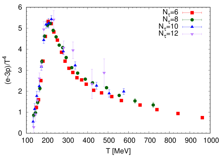
Figure 1: The trace anomaly as function of the temperature calculated on $N_{\tau}=6,~{}8,~{}10$ and $12$ lattices.

As one can see from the figures we have accurate results for the trace anomaly on $N_{\tau}=6$ and $N_{\tau}=8$ lattices. On the other hand there are large fluctuations in the results obtained for $N_{\tau}=10$ and $12$. Nonetheless, there is no apparent cutoff dependence of the trace anomaly for $N_{\tau}>6$. Since we have accurate results for the trace anomaly for $N_{\tau}=6$ and $8$ we interpolate them with splines and then evaluate the pressure via the integral method as discussed above. In Fig. 2 we compare the pressure in (2+1+1)-flavor QCD along the line of constant physics $m_{\pi}\approx 300\,\mathrm{MeV}$ with the pressure in (2+1)-flavor QCD along the line of constant physics $m_{\pi}\approx 160\,\mathrm{MeV}$ [5]. Note that due to the difference in the pion mass for $N_{\tau}=8$ the (2+1+1)-flavor pressure is below the (2+1)-flavor pressure at low temperatures, $T\lesssim 300\,\mathrm{MeV}$, where the contribution of the charm quark is still negligible. For $N_{\tau}=6$ we do not see significant differences since the cutoff effects are more prominent than the quark mass effects.

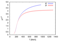
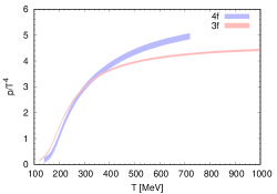
Figure 2: Pressure as function of temperature on $N_{\tau}=6$ (left) and $8$ (right) lattices for (2+1)- and (2+1+1)-flavor QCD. The errors are purely statistical. In the continuum limit, the (2+1)-flavor or (2+1+1)-flavor QCD results correspond to pion masses of $m_{\pi}\approx 160\,\mathrm{MeV}$ or $300\,\mathrm{MeV}$, respectively.

5 Conclusions

We have extended the calculation of the equation of state in (2+1+1)-flavor QCD with HISQ action and concluded the calculation on the coarse lattices. We have generated several new ($T=0$ and $T>0$) ensembles to achieve better coverage of the temperature range 130 - 1000 MeV and increased the statistics on most of the ensembles. We have reached lattice spacings down to $0.034\,\mathrm{fm}$, which corresponds to $967\,\mathrm{MeV}$ for $N_{\tau}=6$. Calculations on $N_{\tau}=6$ and $8$ lattices shows that there is a significant contribution from charm quarks to the pressure for $T>300$ MeV. However, substantial increase in the statistics on the finer ensembles ($N_{\tau}=10,~{}12$) will be needed to accomplish a robust continuum extrapolation.

References

- [1] HotQCD collaboration, A. Bazavov et al., Chiral crossover in QCD at zero and non-zero chemical potentials, Phys. Lett. B 795 (2019) 15 [1812.08235].
- [2] L. Giusti and M. Pepe, Equation of state of the SU(3) Yang–Mills theory: A precise determination from a moving frame, Phys. Lett. B 769 (2017) 385 [1612.00265].
- [3] S. Borsanyi, Z. Fodor, C. Hoelbling, S. D. Katz, S. Krieg and K. K. Szabo, Full result for the QCD equation of state with 2+1 flavors, Phys. Lett. B 730 (2014) 99 [1309.5258].
- [4] HotQCD collaboration, A. Bazavov et al., Equation of state in ( 2+1 )-flavor QCD, Phys. Rev. D 90 (2014) 094503 [1407.6387].
- [5] A. Bazavov, P. Petreczky and J. H. Weber, Equation of State in 2+1 Flavor QCD at High Temperatures, Phys. Rev. D 97 (2018) 014510 [1710.05024].
- [6] S. Borsanyi et al., Calculation of the axion mass based on high-temperature lattice quantum chromodynamics, Nature 539 (2016) 69 [1606.07494].
- [7] P. Petreczky and J. H. Weber, Strong coupling constant from moments of quarkonium correlators revisited, 2012.06193.
- [8] J. Komijani, P. Petreczky and J. H. Weber, Strong coupling constant and quark masses from lattice QCD, Prog. Part. Nucl. Phys. 113 (2020) 103788 [2003.11703].
- [9] M. Laine and Y. Schroder, Quark mass thresholds in QCD thermodynamics, Phys. Rev. D 73 (2006) 085009 [hep-ph/0603048].
- [10] MILC collaboration, A. Bazavov et al., Towards a QCD Equation of State with 2 + 1 + 1 Flavors using the HISQ Action, PoS LATTICE2012 (2012) 071.
- [11] MILC collaboration, A. Bazavov et al., Update on the 2+1+1 Flavor QCD Equation of State with HISQ, PoS LATTICE2013 (2014) 154 [1312.5011].
- [12] HPQCD, UKQCD collaboration, E. Follana, Q. Mason, C. Davies, K. Hornbostel, G. P. Lepage, J. Shigemitsu et al., Highly improved staggered quarks on the lattice, with applications to charm physics, Phys. Rev. D 75 (2007) 054502 [hep-lat/0610092].
- [13] A. Bazavov et al., - and -meson leptonic decay constants from four-flavor lattice QCD, Phys. Rev. D 98 (2018) 074512 [1712.09262].
- [14] MILC collaboration, A. Bazavov et al., Results for light pseudoscalar mesons, PoS LATTICE2010 (2010) 074 [1012.0868].
- [15] G. Boyd, J. Engels, F. Karsch, E. Laermann, C. Legeland, M. Lutgemeier et al., Thermodynamics of SU(3) lattice gauge theory, Nucl. Phys. B 469 (1996) 419 [hep-lat/9602007].
- [16] C. R. Allton, Lattice Monte Carlo data versus perturbation theory, Nucl. Phys. B Proc. Suppl. 53 (1997) 867 [hep-lat/9610014].
- [17] M. A. Clark and A. D. Kennedy, Accelerating dynamical fermion computations using the rational hybrid Monte Carlo (RHMC) algorithm with multiple pseudofermion fields, Phys. Rev. Lett. 98 (2007) 051601 [hep-lat/0608015].