Bias-Variance Tradeoffs in Single-Sample Binary Gradient Estimators

Abstract

Discrete and especially binary random variables occur in many machine learning models, notably in variational autoencoders with binary latent states and in stochastic binary networks. When learning such models, a key tool is an estimator of the gradient of the expected loss with respect to the probabilities of binary variables. The straight-through (ST) estimator gained popularity due to its simplicity and efficiency, in particular in deep networks where unbiased estimators are impractical. Several techniques were proposed to improve over ST while keeping the same low computational complexity: Gumbel-Softmax, ST-Gumbel-Softmax, BayesBiNN, FouST. We conduct a theoretical analysis of bias and variance of these methods in order to understand tradeoffs and verify the originally claimed properties. The presented theoretical results allow for better understanding of these methods and in some cases reveal serious issues.

1 Introduction

Binary variables occur in many models of interest. Variational autoencoders (VAE) with binary latent states are used to learn generative models with compressed representations [10, 11, 22, 33] and to learn binary hash codes for text and image retrieval [6, 30, 7, 20]. Neural networks with binary activations and weights are extremely computationally efficient and attractive for embedded applications, in particular pushed forward in the vision research [12, 8, 25, 3, 34, 36, 1, 15, 2, 31, 4, 17, 5]. Training these discrete models is possible via the stochastic relaxation, equivalent to training a Stochastic Binary Networks (SBN) [23, 24, 29, 26, 27]. In this relaxation, each binary weight is replaced with a Bernoulli random variable and each binary activation is replaced with a conditional Bernoulli variable. The gradient of the expected loss in the weight probabilities is well defined and SGD optimization can be applied.

For the problem of estimating gradient of expectation in probabilities of (conditional) Bernoulli variables, several unbiased estimators were proposed [19, 11, 9, 32, 35]. However, in the context of deep SBNs these methods become impractical: MuProp [11] and reinforce with baselines [19] have a prohibitively high variance in deep layers [28, Figs. C6, C7] while other methods’ complexity grows quadratically with the number of Bernoulli layers. In these cases, biased estimators were more successful in practice: straight-through (ST) [28], Gumbel-Softmax (GS) [13, 16] and their variants. In order to approximate the gradient of the expectation these methods use a single sample of all random entities and the derivative of the objective function extended to the real-valued domain. A more accurate PSA method was presented in [29], which has low computation complexity, but applies only to SBNs of classical structure and requires specialized convolutions. Notably, it was experimentally reported [29, Fig.4] that the baseline ST performs nearly identically to PSA in moderate size SBNs. Fig. 1 schematically illustrates the bias-variance tradeoff with different approaches.

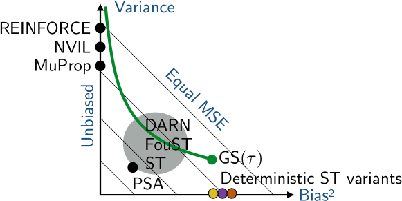
Figure 1: Schematic illustration of bias-variance tradeoffs (we do not pretend on exactness, but see experimental evaluations in [29, 28]; notice that the Mean Squared Error (MSE) is the sum of variance and squared bias). Unbiased methods have a prohibitively high variance for deep models. PSA achieves a significant reduction in variance at a price of a small bias, but has a limited applicability. According to [29], ST estimator can be as accurate as PSA in wide deep models. We analytically study methods in the gray area: GS, DARN and FouST in order to find out whether they can offer a sound improvement over ST. In particular, for GS estimator the figure illustrates its possible tradeoffs when varying the temperature parameter according to the asymptotes we prove.

Contribution

In this work we analyze theoretical properties of several recent single-sample gradient based methods: GS, ST-GS [13], BayesBiNN [18] and FouST [22]. We focus on clarifying these techniques, studying their limitations and identifying incorrect and over-claimed results. We give a detailed analysis of bias and variance of GS and ST-GS estimators. Next we analyze the application of GS in BayesBiNN. We show that a correct implementation would result in an extremely high variance. However due to a hidden issue, the estimator in effect reduces to a deterministic straight-through (with zero variance). A long-range effect of this swap is that BayesBiNN fails to solve the variational Bayesian learning problem as claimed. FouST [22] proposed several techniques for lowering bias and variance of the baseline ST estimator. We show that the baseline ST estimator was applied incorrectly and that some of the proposed improvements may increase bias and or variance.

We believe these results are valuable for researchers interested in applying these methods, working on improved gradient estimators or developing Bayesian learning methods. Incorrect results with hidden issues in the area could mislead many researchers and slow down development of new methods.

Outline

The paper is organized as follows. In Section 2 we briefly review the baseline ST estimator. In the subsequent sections we analyze Gumbel-Softmax estimator (Section 3), BayesBiNN (Section 4) and FouST estimator (Section 5). Proofs are provided in the respective Appendices A to C. As most of our results are theoretical, simplifying derivation or identifying limitations and misspecifications of the preceding work, we do not propose extensive experiments. Instead, we refer to the literature for the experimental evidence that already exists and only conduct specific experimental tests as necessary. In Section 6 we summarize our findings and discuss how they can facilitate future research.

2 Background

We define a stochastic binary unit $x\sim\operatorname*{Bernoulli}(p)$ as $x=1$ with probability $p$ and $x=0$ with probability $1-p$. Let $f(x)$ be a loss function, which in general may depend on other parameters and may be stochastic aside from the dependence on $x$. This is particularly the case when $f$ is a function of multiple binary stochastic variables and we study its dependence on one of them explicitly. The goal of binary gradient estimators is to estimate

$$\textstyle g=\frac{\mathrm{d}}{\mathrm{d}p}{\mathbb{E}}[f(x)],$$ (1)

where ${\mathbb{E}}$ is the total expectation. Gradient estimators which we consider make a stochastic estimate of the total expectation by taking a single joint sample. We will study their properties with respect to $x$ only given the rest of the sample fixed. In particular, we will confine the notion of bias and variance to the conditional expectation ${\mathbb{E}}_{x}$ and the conditional variance $\mathbb{V}_{x}$. We will assume that the function $f(x)$ is defined on the interval $[0,1]$ and is differentiable on this interval. This is typically the case when $f$ is defined as a composition of simple functions, such as in neural networks. While for discrete inputs $x$, the continuous definition of $f$ is irrelevant, it will be utilized by approximations exploiting its derivatives.

The expectation ${\mathbb{E}}_{x}[f(x)]$ can be written as

$$\textstyle(1-p)f(0)+pf(1),$$ (2)

Its gradient in $p$ is respectively

$$\textstyle g=\frac{\mathrm{d}}{\mathrm{d}p}{\mathbb{E}}_{x}[f(x)]=f(1)-f(0).$$ (3)

While this is simple for one random variable $x$, it requires evaluating $f$ at two points. With $n$ binary units in the network, in order to estimate all gradients stochastically, we would need to evaluate the loss $2n$ times, which is prohibitive.

Of high practical interest are stochastic estimators that evaluate $f$ only at a single joint sample (perform a single forward pass). Arguably, the most simple such estimator is the straight-through (ST) estimator:

$$\textstyle\hat{g}_{\text{\sc st}}=f^{\prime}(x).$$ (4)

For an in-depth introduction and more detained study of its properties we refer to [28]. The mean and variance of this ST estimator are given by

$$\textstyle{\mathbb{E}}_{x}[\hat{g}_{\text{\sc st}}] \textstyle=(1-p)f^{\prime}(0)+pf^{\prime}(1),$$ (5a)

$$\textstyle\mathbb{V}_{x}[\hat{g}_{\text{\sc st}}] \textstyle={\mathbb{E}}_{x}[\hat{g}_{\text{\sc st}}^{2}]-({\mathbb{E}}_{x}[\hat{g}_{\text{\sc st}}])^{2}=p(1-p)(f^{\prime}(1)-f^{\prime}(0))^{2}.$$ (5b)

If $f(x)$ is linear in $x$, i.e., $f(x)=hx+c$, where $h$ and $c$ may depend on other variables, then $f^{\prime}(0)=f^{\prime}(1)=h$ and $f(1)-f(0)=h$. In this linear case we obtain

$$\textstyle{\mathbb{E}}_{x}[\hat{g}_{\text{\sc st}}] \textstyle=h,$$ (6a)

$$\textstyle\mathbb{V}_{x}[\hat{g}_{\text{\sc st}}] \textstyle=0.$$ (6b)

From the first expression we see that the estimator is unbiased and from the second one we see that its variance (due to $x$) is zero. It is therefore a reasonable baseline: if $f$ is close to linear, we may expect the estimator to behave well. Indeed, there is a theoretical and experimental evidence [28] that in typical neural networks the more units are used per layer, the closer we are to the linear regime (at least initially) and the better the utility of the estimate for optimization. Furthermore, [29] show that in SBNs of moderate size, the accuracy of ST estimator is on par with a more accurate PSA estimator.

We will study alternative single-sample approaches and improvements proposed to the basic ST. In order to analyze BayesBiNN and FouST we will switch to the $\pm 1$ encoding. We will write $y\sim\operatorname*{Bin}(p)$ to denote a random variable with values $\{-1,1\}$ parametrized by $p=\mathbb{P}_{y}(y{=}1)$. Alternatively, we will parametrize the same distribution using the expectation $\mu=2p-1$ and denote this distribution as $\operatorname*{Bin}(\mu)$ (the naming convention and the context should make it unambiguous). Note that the mean of $\operatorname*{Bernoulli}(p)$ is $p$. The ST estimator of the gradient in the mean parameter $\mu$ in both $\{0,1\}$ and $\{-1,1\}$ valued cases is conveniently given by the same equation (4).

Proof.

Indeed, ${\mathbb{E}}_{y}[f(y)]$ with $y\sim\operatorname*{Bin}(\mu)$ can be equivalently expressed as ${\mathbb{E}}_{x}[\tilde{f}(x)]$ with $x\sim\operatorname*{Bernoulli}(p)$, where $p=\frac{\mu+1}{2}$ and $\tilde{f}(x)=f(2x-1)$. The ST estimator of gradient in the Bernoulli probability $p$ for a sample $x$ can then be written as

$$\textstyle\hat{g}_{\text{\sc st}}=\tilde{f}^{\prime}(x)=2f^{\prime}(y),$$ (7)

where $y=2x-1$ is a sample from $\operatorname*{Bin}(\mu)$. The gradient estimate in $\mu$ becomes $2f^{\prime}(y)\frac{\partial p}{\partial\mu}=f^{\prime}(y)$. ∎

3 Gumbel Softmax and ST Gumbel-Softmax

Gumbel Softmax [13] and Concrete relaxation [16] enable differentiability through discrete variables by relaxing them to real-valued variables that follow a distribution closely approximating the original discrete distribution. The two works [13, 16] have contemporaneously introduced the same relaxation, but the name Gumbel Softmax (GS) became more popular in the literature.

A categorical discrete random variable $x$ with $K$ category probabilities $\pi_{k}$ can be sampled as

$$\textstyle x=\operatorname*{arg\,max}_{k}(\log\pi_{k}-\Gamma_{k}),$$ (8)

where $\Gamma_{k}$ are independent Gumbel noises. This is known as Gumbel reparametrization. In the binary case with categories $k\in\{1,0\}$ we can express it as

$$\textstyle x=\mathchoice{\hbox to0.0pt{$\textstyle{[}$\hss}}{\hbox to0.0pt{$\textstyle{[}$\hss}}{\hbox to0.0pt{$\scriptstyle{[}$\hss}}{\hbox to0.0pt{$\scriptscriptstyle{[}$\hss}}\hskip 1.3pt[\log\pi_{1}-\Gamma_{1}\geq\log\pi_{0}-\Gamma_{0}]\hskip 1.36pt\mathchoice{\hbox to0.0pt{\hss$\textstyle{]}$}}{\hbox to0.0pt{\hss$\textstyle{]}$}}{\hbox to0.0pt{\hss$\scriptstyle{]}$}}{\hbox to0.0pt{\hss$\scriptscriptstyle{]}$}},$$ (9)

where $\mathchoice{\hbox to0.0pt{$\textstyle{[}$\hss}}{\hbox to0.0pt{$\textstyle{[}$\hss}}{\hbox to0.0pt{$\scriptstyle{[}$\hss}}{\hbox to0.0pt{$\scriptscriptstyle{[}$\hss}}\hskip 1.3pt[\cdot]\hskip 1.36pt\mathchoice{\hbox to0.0pt{\hss$\textstyle{]}$}}{\hbox to0.0pt{\hss$\textstyle{]}$}}{\hbox to0.0pt{\hss$\scriptstyle{]}$}}{\hbox to0.0pt{\hss$\scriptscriptstyle{]}$}}$ is the Iverson bracket. More compactly, denoting $p=\pi_{1}$,

$$\textstyle x=\mathchoice{\hbox to0.0pt{$\textstyle{[}$\hss}}{\hbox to0.0pt{$\textstyle{[}$\hss}}{\hbox to0.0pt{$\scriptstyle{[}$\hss}}{\hbox to0.0pt{$\scriptscriptstyle{[}$\hss}}\hskip 1.3pt[\log\frac{p}{1-p}-(\Gamma_{1}-\Gamma_{0})\geq 0]\hskip 1.36pt\mathchoice{\hbox to0.0pt{\hss$\textstyle{]}$}}{\hbox to0.0pt{\hss$\textstyle{]}$}}{\hbox to0.0pt{\hss$\scriptstyle{]}$}}{\hbox to0.0pt{\hss$\scriptscriptstyle{]}$}}.$$ (10)

The difference of two Gumbel variables $z=\Gamma_{1}-\Gamma_{0}$ follows the logistic distribution. Its cdf is $\sigma(z)=\frac{1}{1+e^{-z}}$. Denoting $\eta={\rm logit}(p)$, we obtain the well-known noisy step function representation:

$$\textstyle x=\mathchoice{\hbox to0.0pt{$\textstyle{[}$\hss}}{\hbox to0.0pt{$\textstyle{[}$\hss}}{\hbox to0.0pt{$\scriptstyle{[}$\hss}}{\hbox to0.0pt{$\scriptscriptstyle{[}$\hss}}\hskip 1.3pt[\eta-z\geq 0]\hskip 1.36pt\mathchoice{\hbox to0.0pt{\hss$\textstyle{]}$}}{\hbox to0.0pt{\hss$\textstyle{]}$}}{\hbox to0.0pt{\hss$\scriptstyle{]}$}}{\hbox to0.0pt{\hss$\scriptscriptstyle{]}$}}.$$ (11)

This reparametrization of binary variables is exact but does not yet allow for differentiation of a single sample because we cannot take the derivative under the expectation of this function in (1). The relaxation [13, 16] replaces the threshold function by a continuously differentiable approximation $\sigma_{\tau}(\eta):=\sigma(\eta/\tau)=\frac{1}{1+e^{-\eta/\tau}}$. As the temperature parameter $\tau>0$ decreases towards $0$, the function $\sigma_{\tau}(\eta)$ approaches the step function. The GS estimator of the derivative in $\eta$ is then defined as the total derivative of $f$ at a random relaxed sample:

$$\textstyle z \textstyle\sim\text{Logistic},$$ (12a)

$$\textstyle\tilde{x} \textstyle=\sigma_{\tau}(\eta-z),$$ (12b)

$$\textstyle\frac{\hat{d}f}{d\eta} \textstyle:=\frac{\mathrm{d}f(\tilde{x})}{\mathrm{d}\eta}=f^{\prime}(\tilde{x})\frac{\partial\tilde{x}}{\partial\eta}.$$ (12c)

A possible delusion about GS gradient estimator is that it can be made arbitrary accurate by using a sufficiently small temperature $\tau$. This is however not so simple and we will clarify theoretical reasons for why it is so. An intuitive explanation is proposed in Fig. 2. Formally, we show the following properties.

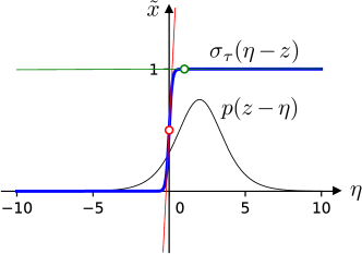
Figure 2: GS Estimator: relaxed samples $\tilde{x}$ are obtained and differentiated as follows. Noisy inputs, following a shifted logistic distribution (black density), are passed through a smoothed step function $\sigma_{\tau}$ (blue). Observe that for a small $\tau$, the derivative is often (in probability of $\eta-z$) close to zero (green) and, very rarely, when $|\eta-z|$ is small, it becomes $O(1/\tau)$ large (red).

Proposition 1.

GS estimator is asymptotically unbiased as $\tau\rightarrow 0$ and the bias decreases at the rate $O(\tau)$ in general and at the rate $O(\tau^{2})$ for linear functions.

Proof in Appendix A. The decrease of the bias with $\tau\rightarrow 0$ is a desirable property, but this advantage is practically nullified by the fast increase of the variance:

Proposition 2.

The variance of GS estimator grows at the rate $O(\frac{1}{\tau})$.

Proof in Appendix A. This fast growth of the variance prohibits the use of small temperatures in practice. In more detail the behavior of the gradient estimator is described by the following two propositions.

Proposition 3.

For any given realization $z\neq\eta$ the norm of GS estimator asymptotically vanishes at the exponential rate $O(\frac{1}{\tau}c^{1/\tau})$ with $c=e^{-|x|}<1$.

Proof in Appendix A. For small $x$, where $c$ is close to one, the term $1/\tau$ dominates at first. In particular for $z=\eta$, the asymptote is $O(1/\tau)$. So while for the most of noise realizations the gradient magnitude vanishes exponentially quickly, it is compensated by a significant grows at rate $1/\tau$ around $z=\eta$. In practice it means that most of the time a value of gradient close to zero is measured and occasionally, very rarely, a value of $O(1/\tau)$ is obtained.

Proposition 4.

The probability to observe GS gradient of norm at least $\varepsilon$ is asymptotically $O(\tau\log(\frac{1}{\varepsilon}))$, where the asymptote is $\tau\rightarrow 0$, $\varepsilon\rightarrow 0$.

Proof in Appendix A.

Unlike ST, GS estimator with $\tau>0$ is biased even for linear objectives. Even for a single neuron and a linear objective it has a non-zero variance. Propositions 3 and 4 apply also to the case of a layer with multiple units since they just analyze the factor $\frac{\partial}{\partial\eta}\sigma_{\tau}(\eta-z)$, which is present independently at all units. Proposition 4 can be extended to deep networks with L layers of Bernoulli variables, in which case the chain derivative will encounter $L$ such factors and we obtain that the probability to observe a gradient with norm at least $\varepsilon$ will vanish at the rate $O(\tau^{L})$.

These facts should convince the reader of the following: it is not possible to use a very small $\tau$, not even with an annealing schedule starting from $\tau=1$. For a very small $\tau$ the most likely consequence would be to never encounter a numerically non-zero gradient during the whole training. For moderately small $\tau$ the variance would be prohibitively high. Indeed, Jang et al. [13] anneal $\tau$ only down to $0.5$ in their experiments.

A major issue with this and other relaxation techniques (i.e. techniques using relaxed samples $\tilde{x}\in\mathbb{R}$) is that the relaxation biases all the expectations. There is only one forward pass and hence the relaxed samples $\tilde{x}$ are used for all purposes, not only for the purpose of estimating the gradient with respect to the given neuron. It biases all expectations for all other units in the same layer as well as in preceding and subsequent layers (in SBN). Let for example $f$ depend on additional parameters $\theta$ in a differentiable way. More concretely, $\theta$ could be parameters of the decoder in VAE. With a Bernoulli sample $x$, an unbiased estimate of gradient in $\theta$ can be obtained simply as $\frac{\partial}{\partial\theta}f(x;\theta)$. However, if we replace the sample with a relaxed sample $\tilde{x}$, the estimate $\frac{\partial}{\partial\theta}f(\tilde{x};\theta)$ becomes biased because the distribution of $\tilde{x}$ only approximates the distribution of $x$. If $y$ were other binary variables relaxed in a similar way, the gradient estimate for $x$ will become more biased because $E_{\tilde{y}}[\nabla_{\tilde{x}}f(\tilde{x},\tilde{y})]$ is a biased estimate of $E_{y}[\nabla_{\tilde{x}}f(\tilde{x},y)]$ desired. Similarly, in a deep SBN, the relaxation applied in one layer of the model additionally biases all expectations for units in layers below and above. In practice the accuracy for VAEs is relatively good [13], [28, Fig. 3] while for deep SBNs a bias higher than of ST is observed for $\tau=1$ in a synthetic model with 2 or more layers and with $\tau=0.1$ for a model with 7 (or more) layers [29, Fig. C.6]. When training moderate size SBNs on real data, it performs worse than ST  [29, Fig. 4].

ST Gumbel-Softmax

Addressing the issue that relaxed variables deviate from binary samples on the forward pass, Jang et al. [13] proposed the following empirical modification. ST Gumbel-Softmax estimator [13] keeps the relaxed sample for the gradient but uses the correct Bernoulli sample on the forward pass:

$$\textstyle z \textstyle\sim\text{Logistic},$$ (13a)

$$\textstyle\tilde{x} \textstyle=\sigma_{\tau}(\eta-z),$$ (13b)

$$\textstyle x \textstyle=\mathchoice{\hbox to0.0pt{$\textstyle{[}$\hss}}{\hbox to0.0pt{$\textstyle{[}$\hss}}{\hbox to0.0pt{$\scriptstyle{[}$\hss}}{\hbox to0.0pt{$\scriptscriptstyle{[}$\hss}}\hskip 1.3pt[\eta-z\geq 0]\hskip 1.36pt\mathchoice{\hbox to0.0pt{\hss$\textstyle{]}$}}{\hbox to0.0pt{\hss$\textstyle{]}$}}{\hbox to0.0pt{\hss$\scriptstyle{]}$}}{\hbox to0.0pt{\hss$\scriptscriptstyle{]}$}},$$ (13c)

$$\textstyle\hat{g}_{\text{\sc st-gs}(\tau)} \textstyle=f^{\prime}(x)\frac{\partial\tilde{x}}{\partial\eta}.$$ (13d)

Note that $x$ is now distributed as $\operatorname*{Bernoulli}(p)$ with $p=\sigma(\eta)$ so the forward pass is fixed. We show the following asymptotic properties.

Proposition 5.

ST Gumbel-Softmax estimator [13] is asymptotically unbiased for quadratic functions and the variance grows as $O(1/\tau)$ for $\tau\rightarrow 0$.

Proof in Appendix A.

To summarize, ST-GS is more expensive than ST as it involves sampling from logistic distribution (and keeping samples), it is biased for $\tau>0$. It becomes unbiased for quadratic functions as $\tau\rightarrow 0$, which would be an improvement over ST, but the variance grows as $\frac{1}{\tau}$.

4 BayesBiNN

Meng et al. [18], motivated by the need to reduce the variance of reinforce, apply GS estimator. However, in their large-scale experiments they use temperature $\tau=10^{-10}$. According to the previous section, the variance of GS estimator should go through the roof as it grows as $O(\frac{1}{\tau})$. It is practically prohibitive as the learning would require an extremely small learning rate and a very long training time as well as high numerical accuracy. Nevertheless, good experimental results are demonstrated [18]. We identify a hidden implementation issue which completely changes the gradient estimator and enables learning.

First, we explain the issue. Meng et al. [18] model stochastic binary weights as $w\sim\operatorname*{Bin}(\mu)$ and express GS estimator as follows.

Proposition 6 (Meng et al. [18] Lemma 1).

Let $w\sim\operatorname*{Bin}(\mu)$ and let $f\colon\{-1,1\}\to\mathbb{R}$ be a loss function. Using parametrization $\mu=\tanh(\lambda)$, $\lambda\in\mathbb{R}$, GS estimator of gradient $\frac{\mathrm{d}{\mathbb{E}}_{w}[f]}{\mathrm{d}\mu}$ can be expressed as

$$\textstyle\delta \textstyle\sim\frac{1}{2}\text{\rm Logistic},$$ (14a)

$$\textstyle\tilde{w} \textstyle=\tanh_{\tau}(\lambda-\delta)\equiv\tanh(\frac{\lambda-\delta}{\tau}),$$ (14b)

$$\textstyle J \textstyle=\frac{1-\tilde{w}^{2}}{\tau(1-\mu^{2})},$$ (14c)

$$\textstyle\hat{g} \textstyle=Jf^{\prime}(\tilde{w}),$$ (14d)

which we verify in Appendix B. However, the actual implementation of the scaling factor $J$ used in the experiments [18] according to the published code introduces a technical $\epsilon=10^{-10}$ as follows:

$$\textstyle J:=\frac{1-\tilde{w}^{2}+\epsilon}{\tau(1-\mu^{2}+\epsilon)}.$$ (15)

It turns out this changes the nature of the gradient estimator and of the learning algorithm. The BayesBiNN algorithm [18, Table 1 middle] performs the update:

$$\textstyle\lambda \textstyle:=(1-\alpha)\lambda-\alpha sf^{\prime}(\tilde{w}),$$ (16)

where $s=NJ$, $N$ is the number of training samples and $\alpha$ is the learning rate.

Proposition 7.

With the setting of the hyper-parameters $\tau=O(10^{-10})$ [18, Table 7] and $\epsilon=10^{-10}$ (author’s implementation) in large-scale experiments (MNIST, CIFAR10, CIFAR100), the BayesBiNN algorithm is practically equivalent to the following deterministic algorithm:

$$\textstyle w \textstyle:=\operatorname*{sign}(\bar{\lambda});$$ (17a)

$$\textstyle\bar{\lambda} \textstyle:=(1-\alpha)\bar{\lambda}-\alpha f^{\prime}(w).$$ (17b)

In particular, it does not depend on the values of $\tau$ and $N$.

Proof in Appendix B. Experimentally, we have verified, using authors implementation, that indeed parameters $\lambda$ (16) grow to the order $10^{10}$ during the first iterations, as predicted by our calculations in the proof.

Notice that the step made in (17b) consists of a decay term $-\alpha\bar{\lambda}$ and the gradient descent term $-\alpha f^{\prime}(w)$, where the gradient $f^{\prime}(w)$ is a straight-through estimate for the deterministic forward pass $w=\operatorname*{sign}(\bar{\lambda})$. Therefore the deterministic ST is effectively used. It is seen that the decay term is the only remaining difference to the deterministic STE algorithm [18, Table 1 left], the method is contrasted to. From the point of view of our study, we should remark that the deterministic ST estimator used in effect indeed decreases the variance (down to zero) however it increases the bias compared to the baseline stochastic ST [28].

The issue has also downstream consequences for the intended Bayesian learning. The claim of Proposition 7 that the method does not depend on $\tau$ and $N$ is perhaps somewhat unexpected, but it makes sense indeed. The initial BayesBiNN algorithm of course depends on $\tau$ and $N$. However due to the issue with the implementation of Gumbel Softmax estimator, for a sufficiently small value of $\tau$ it falls into a regime which is significantly different from the initial Bayesian learning rule and is instead more accurately described by (17). In this regime, the result it produces does not dependent on the particular values of $\tau$ and $N$. While we do not know what problem it is solving in the end, it is certainly not solving the intended variational Bayesian learning problem. This is so because the variational Bayesian learning problem and its solution do depend on $N$ in a critical way. The algorithm Eq. 17 indeed does not solve any variational problem as there is no variational distribution involved (nothing sampled). Yet, the decay term $-\alpha\lambda$ stays effective: if the data gradient becomes small, the decay term implements some small “forgetting” of the learned information and may be responsible for an improved generalization observed in the experiments [18].

5 FouST

Pervez et al. [22] introduced several methods to improve ST estimators using Fourier analyzes of Boolean functions [21] and Taylor series. The proposed methods are guided by this analysis but lack formal guarantees. We study the effect of the proposed improvements analytically.

One issue with the experimental evaluation [22] is that the baseline ST estimator [22, Eq. 7] is misspecified: it is adopted from the works considering $\{0,1\}$ Bernoulli variables without correcting for $\{-1,1\}$ case as in (7), differing by a coefficient $2$. The reason for this misspecifications is that ST is know rather as a folklore, vaguely defined, method (see [28]). While in learning with a simple expected loss this coefficient can be compensated by the tuned learning rate, it can lead to a more serious issues, in particular in VAEs with Bernoulli latents and deep SBNs. VAE training objective [14] has the data evidence part, where binary gradient estimator is required and the prior KL divergence part, which is typically computed analytically and differentiated exactly. Rescaling the gradient of the evidence part only introduces a bias which cannot be compensated by tuning the learning rate. Indeed, it is equivalent to optimizing the objective with the evidence part rescaled. In [28, Fig. 2] we show that this effect is significant. In the reminder of the section we will assume that the correct ST estimator (7) is used as the starting point.

5.1 Lowering Bias by Importance Sampling

The method [22, Sec. 4.1] ”Lowering Bias by Importance Sampling”, as noted by authors, obtains DARN gradient estimator [10, Appendix A] who derived it by applying a (biased) control variate estimate in the reinforce method. Transformed to the encoding with $\pm 1$ variables, it expresses as

$$\textstyle\hat{g}_{\text{\sc darn}}=f^{\prime}(x)/p(x).$$ (18)

By design [10], this method is unbiased for quadratic functions, which is straightforward to verify by inspecting its expectation

$$\textstyle{\mathbb{E}}[\hat{g}_{\text{\sc darn}}]=f^{\prime}(1)+f^{\prime}(0).$$ (19)

While, this is in general an improvement over ST — we may expect that functions close to linear will have a lower bias, it is not difficult to construct an example when it can increase the bias compared to ST.

Example 1.

The method [22, Sec. 4.1] ”Lowering Bias by Importance Sampling”, also denoted as Importance Reweighing (IR), can increase bias.

Let $p\in[0,1]$ and $x\sim\operatorname*{Bin}(p)$. Let $f(x)=|x+a|$. The derivative of ${\mathbb{E}}[f(x)]$ in $p$ is

$$\textstyle\frac{\mathrm{d}}{\mathrm{d}p}((1-p)f(-1)+pf(1))=f(1)-f(-1)=f(1)=2a.$$ (20)

The expectation of $\hat{g}_{\text{\sc st}}$ is given by

$$\textstyle(1-p)2f^{\prime}(-1)+p2f^{\prime}(1)=2(2p-1).$$ (21)

The expectation of $\hat{g}_{\text{\sc darn}}$ is given by

$$\textstyle f^{\prime}(-1)+f^{\prime}(1)=0.$$ (22)

The bias of DARN is $2|a|$ while the bias of ST is $2|a+1-2p|$. Therefore for $a>0$ and $p>0.5$, the bias of DARN estimator is higher. In particular for $a=0.9$ and $p=0.95$ the bias of ST estimator equals $0$ while the bias of DARN estimator equals $1.8$.

Furthermore, we can straightforwardly express its variance.

Proposition 8.

The variance of $\hat{g}_{\text{\sc darn}}$ is expressed as

$$\textstyle\mathbb{V}_{z}[\hat{g}_{\text{\sc darn}}]=\frac{(f^{\prime}(1)-p(f^{\prime}(1)+f^{\prime}(-1)))^{2}}{p(1-p)}.$$ (23)

It has asymptotes $O(\frac{f^{\prime}(-1)^{2}}{1-p})$ for $p\rightarrow 1$ and $O(\frac{f^{\prime}(1)^{2}}{p})$ for $p\rightarrow 0$.

The asymptotes indicate that the variance can grow unbounded for units approaching deterministic mode. If applied in a deep network with $L$ layers, $L$ expressions (18) are multiplied and the variance can grow respectively. Interestingly though, if the probability $p$ is defined using the sigmoid function as $p=\sigma(\eta)$, then the gradient in $\eta$ additionally multiplies by the Jacobian $\sigma^{\prime}(\eta)=p(1-p)$, and the variance of the gradient in $\eta$ becomes bounded. Moreover, a numerically stable implementation can simplify $p(1-p)/p(x)$ for both outcomes of $x$. We conjecture that this estimator can be particularly useful with this parametrization of the probability (which is commonly used in VAEs and SBNs).

Experimental evidence [11, Fig 2.a], where DARN estimator is denoted as “$\frac{1}{2}$” shows that the plain ST performs similar for the structural output prediction problem. However, [11, Fig 3.a] gives a stronger evidence in favor of DARN for VAE. In Fig. 3 we show experiment for the MNIST VAE problem, reproducing the experiment [11, 22] (up to data binarization and implementation details). The exact specification is given in [28, Appendix D.1]. It is seen that DARN improves the training performance compared but needs an earlier stopping and or more regularization. Interestingly, with a correction of accumulated bias using unbiased ARM [35] method with 10 samples, ST leads to better final training and test performance.

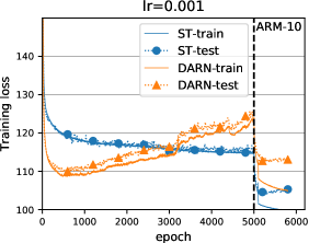
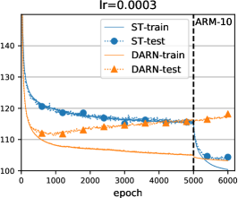
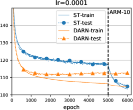
Figure 3: Experimental comparison of DARN and ST estimators on MNIST VAE. The plots show training and test loss (negative ELBO) during training for different learning rates. After 5000 epochs, an unbiased ARM-10 estimator is applied in order to measure (and correct) the accumulated bias. At the smaller learning rates, where DARN does not diverge, it clearly has a much smaller accumulated bias but manages to overfit significantly.

5.2 Reducing Variance via the Fourier Noise Operator

The Fourier noise operator [22, Sec. 2] is defined as follows. For $\rho\in[0,1]$, let $x^{\prime}\sim N_{\rho}(x)$ denote that $x^{\prime}$ is set equal to $x$ with probability $\rho$ and chosen as an independent sample from $\operatorname*{Bin}(p)$ with probability $1-\rho$. The Fourier noise operator smooths the loss function and is defined as $T_{\rho}[f](x)={\mathbb{E}}_{x^{\prime}\sim N_{\rho}(x)}[f(x^{\prime})]$. When applied to $f$ before taking the gradient, it can indeed reduce both bias and variance, ultimately down to zero when $\rho=0$. Indeed, in this case $x^{\prime}$ is independent of $x$ and $T_{\rho}[f](x)={\mathbb{E}}[f(x)]$, which is a constant function of $x$. However, the exact expectation in $x^{\prime}$ is intractable. The computational method proposed in [22, Sec. 4.2] approximates the gradient of this expectation using $S$ samples $x^{(s)}\sim N_{\rho}(x)$ as

$$\textstyle\hat{g}_{\rho}=\frac{1}{S}\sum_{s}\hat{g}(x^{(s)}),$$ (24)

where $\hat{g}$ is the base ST or DARN estimator. We show the following.

Proposition 9.

The method [22, Sec. 4.2] ”Reducing Variance via the Fourier Noise operator” does not reduce the bias (unlike $T_{\rho}$) and increases variance in comparison to the trivial baseline that averages independent samples.

Proof in Appendix C.

This result is found in a sharp contradiction with the experiments [22, Figure 4], where independent samples perform worse than correlated. We do not have a satisfactory explanation for this discrepancy except for the misspecified ST. Since the author’s implementation is not public, it is infeasible to reproduce this experiment in order to verify whether a similar improvement can be observed with the well-specified ST. Lastly, note, that unlike correlated sampling, uncorrelated sampling can be naturally applied with multiple stochastic layers.

5.3 Lowering Bias by Discounting Taylor Coefficients

For the technique [22, Sec. 4.3.1] ”Lowering Bias by Discounting Taylor Coefficients” we present an alternative view, not requiring Taylor series expansion of $f$, thus simplifying the construction. Following [22, Sec. 4.3.1] we assume that the importance reweighing was applied. Since the technique samples $f^{\prime}$ at non-binary points, we refer to it as a relaxed DARN estimator. It can be defined as

$$\textstyle\tilde{g}_{\text{\sc darn}}(x,u)=\frac{f^{\prime}(xu)}{p(x)},\text{where \ }u\sim\mathcal{U}[0,1].$$ (25)

In the total expectation, when we draw $x$ and $u$ multiple times, the gradient estimates are averaged out. The expectation over $u$ alone effectively integrates the derivative to obtain:

$$\textstyle{\mathbb{E}}_{u}\big{[}\tilde{g}_{\text{\sc darn}}(x,u)]=\begin{cases}\frac{1}{p}\int_{0}^{1}f^{\prime}(u)\mathrm{d}u=\frac{1}{p}(f(1)-f(0)),&\text{if\ \ }x=1,\\ \frac{1}{1-p}\int_{0}^{1}f^{\prime}(-u)\mathrm{d}u=\frac{1}{1-p}(f(-1)-f(0)),&\text{if \ }x=-1.\\ \end{cases}$$ (26)

In the expectation over $x$ we therefore obtain

$$\textstyle{\mathbb{E}}_{x,u}[\tilde{g}_{\text{\sc darn}}(x,u)]=f(1)-f(-1),$$ (27)

which is the correct derivative. One issue, discussed by [22] is that variance increases (as there is more noise in the system). However, a major issue similar to GS estimator Section 3, reoccurs here, that all related expectations become biased. In particular (25) becomes biased in the presence of other variables. Pervez et al. [22, Sec. 4.3.1] propose to use $u\in\mathcal{U}[a,1]$ with $a>0$, corresponding to shorter integration intervals around $\pm 1$ states, in order to find an optimal tradeoff.

5.4 Lowering Bias by Representation Rescaling

Consider the estimator $\hat{g}$ of the gradient of function ${\mathbb{E}}_{x}[f(x)]$ where $x\sim\operatorname*{Bin}(p)$. Representation rescaling is defined in [22, Algorithm 1] as drawing $\tilde{x}\sim\frac{1}{\tau}\operatorname*{Bin}(p)$ instead of $x$ and then using FouST estimator based on the derivative $f^{\prime}(\tilde{x})$. It is claimed that using a scaled representation can decrease the bias of the gradient estimate. However, the following issue occurs.

Proposition 10.

The method [22, Sec. 4.3.2] ”Lowering Bias by Representation Rescaling” compares biases of gradient estimators of different functions.

Proof.

Sampling $\tilde{x}$ can be equivalently defined as $\tilde{x}=x/\tau$. Bypassing the analysis of Taylor coefficients [22], it is easy to see that for a smooth function $f$, as $\tau\rightarrow\infty$, $f(x/\tau)$ approaches a linear function of $x$ and therefore the bias of the ST estimator of ${\mathbb{E}}_{x}[f(x/\tau)]$ approaches zero. However, clearly ${\mathbb{E}}_{x}[f(x/\tau)]$ is a different function from ${\mathbb{E}}_{x}[f(x)]$ which we wish to optimize. ∎

We explain, why this method nevertheless has effect. Choosing and fixing the scaling hyper-parameter $\tau$ is equivalent to staring from a different initial point, where (initially random) weights are scaled by $1/\tau$. At this initial point, the network is found to be closer to a linear regime, where the ST estimator is more accurate and possibly the vanishing gradient issue is mitigated. Thus the method can have a positive effect on the learning as observed in [22, Appendix Table 3].

6 Conclusion

We theoretically analyzed properties of several methods for estimation of binary gradients and gained interesting new insights.

• For GS and ST-GS estimator we proposed a simplified presentation for the binary case and explained detrimental effects of low and high temperatures. We showed that bias of ST-GS estimator approaches that of DARN, connecting these two techniques.

• For BayesBiNN we identified a hidden issue that completely changes the behavior of the method from the intended variational Bayesian learning with Gumbel-Softmax estimator, theoretically impossible due to the used temperature $\tau=10^{-10}$, to non-Bayesian learning with deterministic ST estimator and latent weight decay. As this learning method shows improved experimental results, it becomes an open problem to clearly understand and advance the mechanism which facilitates this.

• In our analysis of techniques comprising FouST estimator, we provided additional insights and showed that some of these techniques are not well justified. It remains open, whether they are nevertheless efficient in practice in some cases for other unknown reasons, not taken into account in this analysis.

Overall we believe our analysis clarifies the surveyed methods and uncovers several issues which limit their applicability in practice. It provides tools and clears the ground for any future research which may propose new improvements and would need to compare with existing methods both theoretically and experimentally. We hope that this study will additionally motivate such research.

Appendix

Appendix 0.A Gumbel Softmax and ST Gumbel-Softmax

See 1

Proof.

Let us denote

$$\textstyle\bar{g}_{\tau}={\mathbb{E}}_{z}[\hat{g}_{\text{\sc gs}(\tau)}]=\int_{-\infty}^{\infty}\frac{d}{d\eta}f(\sigma_{\tau}(\eta-z))p_{z}(z)\mathrm{d}z.$$ (28)

Note that $\lim_{\tau\rightarrow 0+}\bar{g}_{\tau}(x)$ cannot be simply be evaluated by moving the limit under the integral — no qualification theorem allows this. We apply the following reformulation. The derivative $\frac{d}{d\eta}f(\sigma_{\tau}(\eta-z))$ expands as

$$\textstyle f^{\prime}(\sigma_{\tau}(\eta-z))\sigma_{\tau}(\eta-z)(1-\sigma_{\tau}(\eta-z))\frac{1}{\tau}.$$ (29)

We make a change of variables $v=\sigma_{\tau}(\eta-z)$ in the integral. This gives $z=\eta-\tau{\rm logit}(v)$ and $\mathrm{d}z=-\tau\frac{1}{v(1-v)}\mathrm{d}v$. Substituting and cancelling part of the terms, we obtain

$$\textstyle\bar{g}_{\tau}=\int_{0}^{1}f^{\prime}(v)p_{z}(\eta-\tau{\rm logit}(v))\mathrm{d}v.$$ (30)

With this expression we can now interchange the limit and the integral using the dominated convergence theorem. In order to apply it we need to show that there exist an integrable function $h(v)$ such that

$$\textstyle|f^{\prime}(v)p_{z}(\eta-\tau{\rm logit}(v))|<h(v)$$ (31)

for all $\tau>0$. Observe that

$$\textstyle\sup_{v\in[0,1]}|p_{z}(\eta-\tau{\rm logit}(v))|=\sup_{u\in\mathbb{R}}|p_{z}(\eta-\tau u)|=\sup_{y\in\mathbb{R}}|p_{z}(y)|=p_{z}(0)=\frac{1}{4},$$ (32)

where we used that the maximum of standard logistic density is attained at zero. We can therefore let $h(v)=f^{\prime}(v)/4$. Since $f^{\prime}(v)$ is the derivative of $f$, it is integrable on $[0,1]$. Therefore the conditions of the dominated convergence theorem are satisfied and we have

$$\textstyle\lim_{\tau\rightarrow 0+}\bar{g}_{\tau} \textstyle=\int_{0}^{1}f^{\prime}(v)\lim_{\tau\rightarrow 0+}p_{z}(\eta-\tau{\rm logit}(v))\mathrm{d}v$$ (33a)

$$\textstyle=\int_{0}^{1}f^{\prime}(v)p_{z}(\eta)\mathrm{d}v=(f(1)-f(0))p_{z}(\eta),$$ (33b)

which is the correct value of the gradient in $\eta$.

Next, we obtain the series representation of the estimator bias in the asymptote $\tau\rightarrow 0$. We approximate $p_{z}(\eta-\tau{\rm logit}(v))$ with its Taylor series around $\tau=0$:

$$\textstyle p_{z}(\eta-\tau{\rm logit}(v))=p_{z}(\eta)\Big{(}1+c_{1}{\rm logit}(v)\tau+c_{2}{\rm logit}^{2}(v)\tau^{2}+O(\tau^{3})\Big{)},$$ (34)

where

$$\textstyle c_{1}=\frac{e^{\eta}-1}{e^{\eta}+1};\ \ \ \ \ c_{2}=\frac{-4e^{\eta}+e^{2\eta}+1}{2(e^{\eta}+1)^{2}}.$$ (35)

This is obtained using Mathematica. We use this expansion in the integral representation Eq. 30. Observing that $\int_{0}^{1}f^{\prime}(v)\mathrm{d}v=(f(1)-f(0))$ is the true gradient, the zero order term becomes the true gradient. It follows that the bias of $\hat{g}_{\text{\sc gs}(\tau)}$ is asymptotically

$$\textstyle p_{z}(\eta)\Big{(}c_{1}\Big{(}\int_{0}^{1}f^{\prime}(v){\rm logit}(v)\mathrm{d}v\Big{)}\tau+c_{2}\Big{(}\int_{0}^{1}f^{\prime}(v){\rm logit}^{2}(v)\mathrm{d}v\Big{)}\tau^{2}\Big{)}+O(\tau^{3}).$$ (36)

In the case when $f$ is linear, the first order term vanishes because $f^{\prime}$ is constant and ${\rm logit}(v)$ is odd about $\tfrac{1}{2}$. However $\tau^{2}$ and higher order even terms do not vanish, therefore the estimator is still biased even for linear objectives. ∎

See 2

Proof.

We will show that the second moment of the estimator $\hat{g}_{\text{\sc gs}(\tau)}$ has the following asymptotic expansion for $\tau\rightarrow 0$:

$$\textstyle p_{z}(\eta)\Big{[}\Big{(}\int_{0}^{1}f^{\prime}(v)^{2}v(1-v)\Big{)}\frac{1}{\tau}+ \textstyle c_{1}\Big{(}\int_{0}^{1}f^{\prime}(v)^{2}v(1-v){\rm logit}(v)\mathrm{d}v\Big{)}$$

$$\textstyle+ \textstyle c_{2}\Big{(}\int_{0}^{1}f^{\prime}(v)^{2}v(1-v){\rm logit}^{2}(v)\mathrm{d}v\Big{)}\tau\Big{]}+O(\tau^{2}).$$ (37)

The second moment expresses as

$$\textstyle{\mathbb{E}}[\hat{g}_{\text{\sc gs}(\tau)}^{2}] \textstyle=\int_{-\infty}^{\infty}(\frac{\partial}{\partial\eta}f(\sigma_{\tau}(\eta-z)))^{2}p_{z}(z)\mathrm{d}z$$ (38a)

$$\textstyle=\int_{-\infty}^{\infty}\Big{(}f^{\prime}(\sigma_{\tau}(\eta-z))\sigma_{\tau}(\eta-z)(1-\sigma_{\tau}(\eta-z))\frac{1}{\tau}\Big{)}^{2}p_{z}(z)dz$$ (38b)

We perform the same substitution of variables: $v=\sigma_{t}(\eta-z)$, $dv=-v(1-v)\frac{1}{\tau}\mathrm{d}z$ to obtain

$$\textstyle{\mathbb{E}}[\hat{g}_{\text{\sc gs}(\tau)}^{2}]=\frac{1}{\tau}\int_{0}^{1}f^{\prime}(v)^{2}v(1-v)p_{z}(\eta-\tau{\rm logit}(v))\mathrm{d}v.$$ (39)

We perform the same Taylor expansion for $p_{z}(\eta-\tau{\rm logit}(v))$ around $\tau=0$ as in Proposition 1 and combine the terms to obtain the expansion (37). The variance is dominated by the $O(\tfrac{1}{\tau})$ term of the second moment. ∎

See 3

Proof.

Considering $z$ fixed and denoting $x=\eta-z$, we need to check the asymptotic behavior of

$$\textstyle\frac{\mathrm{d}}{\mathrm{d}x}\sigma_{\tau}(x)=\frac{1}{\tau}p_{z}(x/\tau)=\frac{e^{-\frac{x}{\tau}}}{\tau(1+e^{-x/\tau})^{2}}$$ (40)

as $\tau\rightarrow 0$. Since $p_{z}$ is symmetric, we may assume $x>0$ without loss of generality. The denominator is then asymptotically just $\tau$. Therefore the ratio is asymptotically $O(\frac{1}{\tau}c^{1/\tau})$. ∎

See 4

Proof.

We want to analyze the probability

$$\textstyle P=\mathbb{P}(\frac{\mathrm{d}}{\mathrm{d}\eta}\sigma_{\tau}(\eta-z)\geq\varepsilon)$$ (41)

when $z$ is distributed logistically. Let $s=\sigma_{\tau}(\eta-z)$. Then $\frac{\mathrm{d}}{\mathrm{d}\eta}\sigma_{\tau}(\eta-z)=s(1-s)$. The equality $s(1-s)=\varepsilon$ holds for $s^{*}=\tfrac{1}{2}(1-\sqrt{1-4\varepsilon})$. This implies

$$\textstyle z_{1,2}=\eta\pm\tau{\rm logit}(s^{*}).$$ (42)

The inequality $s(1-s)\geq\varepsilon$ holds in the interval $[z_{1},z_{2}]$. Thus the probability in question is given by

$$\textstyle P=\sigma(z_{2})-\sigma(z_{1}).$$ (43)

As $\tau{\rm logit}(s^{*})\rightarrow 0$ for $\tau\rightarrow 0$, we have asymptotically that

$$\textstyle P=p_{z}(\eta)\tau{\rm logit}(s^{*}).$$ (44)

Finally, note that ${\rm logit}(\tfrac{1}{2}(1-\sqrt{1-4\varepsilon}))$ is asymptotically $O(-\log\varepsilon)$ for $\varepsilon\rightarrow 0$. ∎

See 5

Proof.

Notice that the derivative $f^{\prime}(x)$ in ST-GS only takes two values: $f^{\prime}(1)$ for $\eta-z\geq 0$ and $f^{\prime}(0)$ otherwise. Introducing $v=\tau\sigma_{\tau}(\eta-z)$, the condition $\eta\geq z$ can be equivalently written as $\eta\geq\eta-\tau{\rm logit}(v)$, which reduces to $v\leq 0.5$. In the expected GS gradient value we can therefore substitute

$$\textstyle\begin{cases}f^{\prime}(v)=f^{\prime}(1)&\text{\ if \ \ }v\leq 0.5,\\ f^{\prime}(v)=f^{\prime}(0)&\text{\ otherwise},\end{cases}$$ (45)

and obtain for the expected value of the estimate

$$\textstyle\bar{g}_{\tau}=f^{\prime}(1)\int_{0}^{0.5}p_{z}(\eta-\tau{\rm logit}(v))\mathrm{d}v+f^{\prime}(0)\int_{0.5}^{1}p_{z}(\eta-\tau{\rm logit}(v))\mathrm{d}v.$$ (46)

Substituting the Taylor expansion of $p_{z}(\eta-\tau{\rm logit}(v))$ in $\tau$, we obtain

$$\textstyle\bar{g}_{\tau}=p_{z}(\eta)\Big{(}(f^{\prime}(1)+f^{\prime}(0))\frac{1}{2}+(f^{\prime}(0)-f^{\prime}(0))c_{1}\log(2)\tau\Big{)}+O(\tau^{2}).$$ (47)

We see that in the asymptote $\tau\rightarrow 0$, the expected value of the estimator approaches $p_{z}(\eta)(f^{\prime}(1)+f^{\prime}(0))\frac{1}{2}$, which matches the DARN estimator (confer to (19), which is the expected DARN gradient in $p$ for $\{-1,1\}$ variables, while $g_{\tau}$ is in $\eta$ and $\{0,1\}$ variables). Therefore, bias, approaches that of DARN, in particular the bias vanishes for quadratic $f$. Indeed, let $f(x)=ax^{2}+bx+c$, then the correct gradient is $p_{z}(\eta)(a+b)$.

The variance of ST GS estimator is dominated by the second moment, which has asymptotic expansion (39) with the substitution (45). The variance is dominated by the $O(\tfrac{1}{\tau})$ term of the second moment. More specifically we have the asymptote of the second moment

$$\textstyle\frac{1}{\tau}\Big{(}f^{\prime}(1)^{2}+f^{\prime}(0)^{2}\Big{)}\frac{1}{12}+\Big{(}f^{\prime}(1)^{2}-f^{\prime}(0)^{2}\Big{)}\frac{1-4\log(2)}{24}+O(\tau).$$ (48)

∎

Appendix 0.B BayesBiNN

See 6

Proof.

This result is already proven in Meng et al. [18, Lemma 1]. We nevertheless repeat the derivation in order to make sure there is no mismatch due to a different notation and in order to expand proof details omitted in [18].

Recall that $\tanh(\lambda)=2\sigma(2\lambda)-1$. Let us define $x=(w+1)/2$, $p=(\mu+1)/2$, $\tilde{f}\colon\{0,1\}\mapsto\mathbb{R}\colon x\to f(2x-1)$ and $\eta=2\lambda$. We have $x\sim\operatorname*{Bernoulli}(p)$, $p=\sigma(\eta)$ and ${\mathbb{E}}_{w}[f(w)]={\mathbb{E}}_{x}[\tilde{f}(x)]=:E$. According to (12), the GS estimate of gradient of $E$ in $\eta$ is given by

$$\textstyle z \textstyle\sim\text{Logisitc},$$ (49a)

$$\textstyle\tilde{x} \textstyle=\sigma_{\tau}(\eta-z),$$ (49b)

$$\textstyle\frac{\hat{\mathrm{d}}E}{d\eta} \textstyle=\tilde{f}^{\prime}(\tilde{x})\frac{\partial\tilde{x}}{\partial\eta}.$$ (49c)

Defining $\tilde{w}=2\tilde{x}-1$ and back-substituting, we obtain

$$\textstyle\tilde{w} \textstyle=\tanh_{\tau}(\frac{\eta-z}{2})=\tanh_{\tau}(\lambda-z/2),$$ (50a)

$$\textstyle\frac{\hat{\mathrm{d}}E}{d\lambda}=2\frac{\hat{\mathrm{d}}E}{d\eta} \textstyle=2\Big{(}2f^{\prime}(\tilde{w})\Big{)}\Big{(}\frac{1}{4}\frac{\partial\tilde{w}}{\partial\lambda}\Big{)}=f^{\prime}(\tilde{w})\frac{\partial\tilde{w}}{\partial\lambda}.$$ (50b)

Respectively, GS estimator of gradient $\frac{\mathrm{d}{\mathbb{E}}_{w}[f]}{\mathrm{d}\mu}$ is given by

$$\textstyle\hat{g}=f^{\prime}(\tilde{w})\frac{\partial\tilde{w}}{\partial\lambda}\Big{(}\frac{\partial\mu}{\partial\lambda}\Big{)}^{-1}.$$ (51)

Using the identity $\frac{\mathrm{d}}{\mathrm{d}x}\tanh(x)=1-\tanh^{2}(x)$, we obtain

$$\textstyle\hat{g}=f^{\prime}(\tilde{w})\frac{1-\tilde{w}^{2}}{\tau(1-\mu^{2})}.$$ (52)

Finally note that $z/2\sim\frac{1}{2}\text{Logistic}$. ∎

See 7

Proof.

First, we analyze the nominator of J (15). From the asymptotic expansion of

$$\textstyle 1-\tanh[\log(x)]^{2}=\frac{4}{x^{2}}+O(\frac{1}{x^{3}}),\text{for\ }x\rightarrow\infty,$$ (53)

substituting $\log(x)=\frac{|\lambda-\delta|}{\tau}$, we obtain

$$\textstyle 1-\tilde{w}^{2}\sim 4\exp\big{(}-2\frac{|\lambda-\delta|}{\tau}\big{)}.$$ (54)

For example, for $\lambda=5$ and $\delta=0$ we have that $(1-\tilde{w}^{2})\approx 4e^{-10^{11}}$. Therefore in the nominator, the part $(1-\tilde{w}^{2})$ is negligibly small compared to $\varepsilon$ and even to the floating point precision. This applies so long as $|\lambda-\delta|\gg\tau=10^{-10}$, which we expect to hold with high probability for two reasons: 1) $\lambda$ will be shown to grow significantly during the first iterates and 2) the probability of the noise $\delta$ matching $\lambda$ to this accuracy even for $\lambda=0$ is of the order $O(\tau)$.

The denominator of J (15) satisfies the bounds

$$\textstyle\tau\epsilon\leq\tau(1-\tanh(\lambda)^{2}+\epsilon)\leq\tau(1+\epsilon),$$ (55)

from which we can conclude that $J\geq\frac{\varepsilon}{\tau}=1$. However for a moderately large $\lambda$ the denominator drops quickly, e.g. for $\lambda=5$, we have $\tau(1-\tanh(\lambda)^{2}+\varepsilon)<\tau(2\cdot 10^{-4}+\varepsilon)\approx 2\cdot 10^{-4}\tau$. And the decrease rate for $|\lambda|\rightarrow\infty$ is $\tau(4e^{-2|\lambda|}+\epsilon)$.

Since $\lambda$ is initialized uniformly in $[-10,10]$ and receives updates of order at least $\alpha Nf^{\prime}\approx 5f^{\prime}$ (for the initial $\alpha=10^{-4}$ used), during the first iterates $|\lambda|$ can be expected to grow significantly until we reach the asymptote $e^{-2|\lambda|}\ll\varepsilon$, which is when $|\lambda|>5\log 10\approx 11$. After reaching this asymptote, we will have $J\approx\frac{\epsilon}{\tau\epsilon}=\frac{1}{\tau}$ and we may expect the growth of $\lambda$ to stabilize around $|\lambda|\approx\alpha\frac{N}{\tau}|f^{\prime}|\approx 10^{10}$.

The first consequence of this is that the scaling factor that was supposed to implement Gumbel-Softmax gradient, just becomes an inadvertent constant $\frac{1}{\tau}$.

The second consequence is that the natural parameters $\lambda$ have huge magnitudes during the training, and we have that $|\delta|\ll|\lambda|$ with high probability, therefore the noise plays practically no role even in the forward pass of BayesBiNN. In this mode the BayesBiNN algorithm becomes equivalent to

$$\textstyle w \textstyle:=\operatorname*{sign}(\lambda);$$ (56a)

$$\textstyle\lambda \textstyle:=(1-\alpha)\lambda-\alpha\frac{N}{\tau}f^{\prime}(w).$$ (56b)

It is seen that the forward pass and the gradient implement the deterministic straight-through with identity derivative and that the update has a form of SGD with a latent weight decay and with the gradient of data evidence up-scaled by $\frac{1}{\tau}$. These huge step-sizes of $O(\frac{1}{\tau})$ do not destroy the learning because $\operatorname*{sign}$ is invariant to a global rescaling of $\lambda$.

Denoting $\bar{\lambda}=\frac{\tau}{N}\lambda$, we can equivalently rewrite (56) as

$$\textstyle w \textstyle:=\operatorname*{sign}(\bar{\lambda});$$ (57a)

$$\textstyle\bar{\lambda} \textstyle:=(1-\alpha)\bar{\lambda}-\alpha f^{\prime}(w).$$ (57b)

This algorithm and the resulting binary weights $w$ do not depend on $\tau$, $N$. ∎

Appendix 0.C FouST

See 9

Proof.

We have

$$\textstyle{\mathbb{E}}[\hat{g}_{\rho}] \textstyle={\mathbb{E}}_{x}\Big{[}\frac{1}{S}\sum_{s}{\mathbb{E}}_{x^{\prime}\sim N_{\rho}(x)}[\hat{g}(x^{\prime})]\Big{]}$$ (58a)

$$\textstyle={\mathbb{E}}_{x}\Big{[}\frac{1}{S}\sum_{s}(\rho\hat{g}(x)+(1-\rho){\mathbb{E}}_{x^{\prime}}[\hat{g}(x^{\prime})])\Big{]}={\mathbb{E}}[\hat{g}]=:\mu,$$ (58b)

where ${\mathbb{E}}_{x^{\prime}}$ denotes samples from the base distribution $\operatorname*{Bin}(p)$. Therefore this estimator, unlike the motivating operator $T_{\rho}[f](x)$, does not reduce the bias, no matter how many samples we use. We can express the variance as

$$\textstyle\mathbb{V}[\hat{g}_{\rho}]={\mathbb{E}}[\hat{g}_{\rho}^{2}]-\mu^{2}$$ (59)

$$\textstyle={\mathbb{E}}\big{[}\big{(}\frac{1}{S}\sum_{s}\hat{g}(x^{(s)})\big{)}^{2}\big{]}-{\mathbb{E}}[\hat{g}(x)^{2}]$$ (60)

$$\textstyle=\frac{1}{S}M+\frac{1}{S^{2}}{\mathbb{E}}\big{[}\sum_{s\neq t}\hat{g}(x^{(s)})\hat{g}(x^{(t)})\big{]}-\mu^{2},$$ (61)

where $M={\mathbb{E}}\big{[}\hat{g}(x)^{2}\big{]}$ and further expand

$$\textstyle\frac{1}{S^{2}}{\mathbb{E}}\big{[}\sum_{s\neq t}\hat{g}(x^{(s)})\hat{g}(x^{(t)})\big{]}=$$ (62)

$$\textstyle\frac{1}{S^{2}}{\mathbb{E}}_{x,x^{\prime},x^{\prime\prime}}\big{[}\sum_{s\neq t}(\rho\hat{g}(x)+(1-\rho)\hat{g}(x^{\prime}))(\rho\hat{g}(x)+(1-\rho)\hat{g}(x^{\prime\prime}))\big{]}$$ (63)

$$\textstyle=\frac{1}{S^{2}}{\mathbb{E}}_{x,x^{\prime},x^{\prime\prime}}\big{[}\sum_{s\neq t}(\rho^{2}\hat{g}(x)^{2}+2\rho(1-\rho)\hat{g}(x^{\prime})\hat{g}(x)+(1-\rho)^{2}\hat{g}(x^{\prime})\hat{g}(x^{\prime\prime}))\big{]}$$ (64)

$$\textstyle=\frac{S-1}{S}\Big{(}\rho^{2}{\mathbb{E}}_{x}\big{[}(\hat{g}(x)^{2}]+(2\rho(1-\rho)+(1-\rho)^{2})({\mathbb{E}}_{z}[\hat{g}(x)])^{2}\Big{)}$$ (65)

$$\textstyle=\frac{S-1}{S}\Big{(}\rho^{2}{\mathbb{E}}_{x}\big{[}(\hat{g}(x)^{2}]+(-2\rho^{2}+1+\rho^{2})({\mathbb{E}}_{z}[\hat{g}(x)])^{2}\Big{)}$$ (66)

$$\textstyle=\frac{S-1}{S}\Big{(}\rho^{2}M+(1-\rho^{2})\mu^{2}\Big{)}.$$ (67)

In total we obtain:

$$\textstyle\mathbb{V}[\hat{g}_{\rho}]=\frac{1}{S}\Big{(}(1+(S-1)\rho^{2})M+((S-1)(1-\rho^{2})-S)\mu^{2}\Big{)}.$$ (68)

Respectively,

$$\textstyle\mathbb{V}[\hat{g}_{\rho}]-\mathbb{V}[\hat{g}_{0}]=\frac{S-1}{S}\rho^{2}\sigma^{2}.$$ (69)

This shows that variance using correlated samples is always higher. ∎

References

- Alizadeh et al. [2019] Alizadeh, M., Fernandez-Marques, J., Lane, N. D., and Gal, Y. An empirical study of binary neural networks’ optimisation. In ICLR, 2019.
- Bethge et al. [2019] Bethge, J., Yang, H., Bornstein, M., and Meinel, C. Back to simplicity: How to train accurate BNNs from scratch? CoRR, abs/1906.08637, 2019.
- Bulat & Tzimiropoulos [2017] Bulat, A. and Tzimiropoulos, G. Binarized convolutional landmark localizers for human pose estimation and face alignment with limited resources. In ICCV, Oct 2017.
- Bulat et al. [2019] Bulat, A., Tzimiropoulos, G., Kossaifi, J., and Pantic, M. Improved training of binary networks for human pose estimation and image recognition. arXiv, 2019.
- Bulat et al. [2021] Bulat, A., Martinez, B., and Tzimiropoulos, G. High-capacity expert binary networks. In ICLR, 2021.
- Chaidaroon & Fang [2017] Chaidaroon, S. and Fang, Y. Variational deep semantic hashing for text documents. In SIGIR Conference on Research and Development in Information Retrieval, pp. 75–84, 2017.
- Dadaneh et al. [2020] Dadaneh, S. Z., Boluki, S., Yin, M., Zhou, M., and Qian, X. Pairwise supervised hashing with Bernoulli variational auto-encoder and self-control gradient estimator. ArXiv, abs/2005.10477, 2020.
- Esser et al. [2016] Esser, S. K., Merolla, P. A., Arthur, J. V., Cassidy, A. S., Appuswamy, R., Andreopoulos, A., Berg, D. J., McKinstry, J. L., Melano, T., Barch, D. R., di Nolfo, C., Datta, P., Amir, A., Taba, B., Flickner, M. D., and Modha, D. S. Convolutional networks for fast, energy-efficient neuromorphic computing. Proceedings of the National Academy of Sciences, 113(41):11441–11446, 2016.
- Grathwohl et al. [2018] Grathwohl, W., Choi, D., Wu, Y., Roeder, G., and Duvenaud, D. Backpropagation through the void: Optimizing control variates for black-box gradient estimation. In ICLR, 2018.
- Gregor et al. [2014] Gregor, K., Danihelka, I., Mnih, A., Blundell, C., and Wierstra, D. Deep autoregressive networks. In ICML, 2014.
- Gu et al. [2016] Gu, S., Levine, S., Sutskever, I., and Mnih, A. Muprop: Unbiased backpropagation for stochastic neural networks. In 4th International Conference on Learning Representations (ICLR), May 2016.
- Horowitz [2014] Horowitz, M. Computing’s energy problem (and what we can do about it). In International Solid-State Circuits Conference Digest of Technical Papers (ISSCC), pp. 10–14, 2014.
- Jang et al. [2017] Jang, E., Gu, S., and Poole, B. Categorical reparameterization with gumbel-softmax. In ICLR, 2017.
- Kingma & Welling [2013] Kingma, D. P. and Welling, M. Auto-encoding variational Bayes. CoRR, abs/1312.6114, 2013.
- Liu et al. [2018] Liu, Z., Wu, B., Luo, W., Yang, X., Liu, W., and Cheng, K.-T. Bi-real net: Enhancing the performance of 1-bit CNNs with improved representational capability and advanced training algorithm. In ECCV, pp. 722–737, 2018.
- Maddison et al. [2017] Maddison, C. J., Mnih, A., and Teh, Y. W. The concrete distribution: A continuous relaxation of discrete random variables. In ICLR, 2017.
- Martínez et al. [2020] Martínez, B., Yang, J., Bulat, A., and Tzimiropoulos, G. Training binary neural networks with real-to-binary convolutions. In ICLR, 2020.
- Meng et al. [2020] Meng, X., Bachmann, R., and Khan, M. E. Training binary neural networks using the Bayesian learning rule. In ICML, 2020.
- Mnih & Gregor [2014] Mnih, A. and Gregor, K. Neural variational inference and learning in belief networks. In ICML, volume 32 of JMLR Proceedings, pp. 1791–1799, 2014.
- Ñanculef et al. [2020] Ñanculef, R., Mena, F. A., Macaluso, A., Lodi, S., and Sartori, C. Self-supervised bernoulli autoencoders for semi-supervised hashing. CoRR, abs/2007.08799, 2020.
- O’Donnell [2014] O’Donnell, R. Analysis of Boolean Functions. Cambridge University Press, USA, 2014. ISBN 1107038324.
- Pervez et al. [2020] Pervez, A., Cohen, T., and Gavves, E. Low bias low variance gradient estimates for boolean stochastic networks. In ICML, volume 119, pp. 7632–7640, 13–18 Jul 2020.
- Peters & Welling [2018] Peters, J. W. and Welling, M. Probabilistic binary neural networks. arXiv preprint arXiv:1809.03368, 2018.
- Raiko et al. [2015] Raiko, T., Berglund, M., Alain, G., and Dinh, L. Techniques for learning binary stochastic feedforward neural networks. In ICLR, 2015.
- Rastegari et al. [2016] Rastegari, M., Ordonez, V., Redmon, J., and Farhadi, A. XNOR-Net: Imagenet classification using binary convolutional neural networks. In ECCV, pp. 525–542. Springer, 2016.
- Roth et al. [2019] Roth, W., Schindler, G., Fröning, H., and Pernkopf, F. Training discrete-valued neural networks with sign activations using weight distributions. In European Conference on Machine Learning (ECML), 2019.
- Shayer et al. [2018] Shayer, O., Levi, D., and Fetaya, E. Learning discrete weights using the local reparameterization trick. In ICLR, 2018.
- Shekhovtsov & Yanush [2021] Shekhovtsov, A. and Yanush, V. Reintroducing straight-through estimators as principled methods for stochastic binary networks. In GCPR, 2021.
- Shekhovtsov et al. [2020] Shekhovtsov, A., Yanush, V., and Flach, B. Path sample-analytic gradient estimators for stochastic binary networks. In NeurIPS, 2020.
- Shen et al. [2018] Shen, D., Su, Q., Chapfuwa, P., Wang, W., Wang, G., Henao, R., and Carin, L. NASH: Toward end-to-end neural architecture for generative semantic hashing. In Annual Meeting of the Association for Computational Linguistics, 2018.
- Tang et al. [2017] Tang, W., Hua, G., and Wang, L. How to train a compact binary neural network with high accuracy? In AAAI, 2017.
- Tucker et al. [2017] Tucker, G., Mnih, A., Maddison, C. J., Lawson, J., and Sohl-Dickstein, J. REBAR: Low-variance, unbiased gradient estimates for discrete latent variable models. In NeurIPS, 2017.
- Vahdat et al. [2020] Vahdat, A., Andriyash, E., and Macready, W. Undirected graphical models as approximate posteriors. In ICML, volume 119, pp. 9680–9689, 13–18 Jul 2020.
- Xiang et al. [2017] Xiang, X., Qian, Y., and Yu, K. Binary deep neural networks for speech recognition. In INTERSPEECH, 2017.
- Yin & Zhou [2019] Yin, M. and Zhou, M. ARM: Augment-REINFORCE-merge gradient for stochastic binary networks. In ICLR, 2019.
- Zhou et al. [2016] Zhou, S., Wu, Y., Ni, Z., Zhou, X., Wen, H., and Zou, Y. Dorefa-net: Training low bitwidth convolutional neural networks with low bitwidth gradients. arXiv preprint arXiv:1606.06160, 2016.