Prototype Learning for Interpretable Respiratory Sound Analysis

Abstract

Remote screening of respiratory diseases has been widely studied as a non-invasive and early instrument for diagnosis purposes, especially in the pandemic. The respiratory sound classification task has been realized with numerous deep neural network (DNN) models due to their superior performance. However, in the high-stake medical domain where decisions can have significant consequences, it is desirable to develop interpretable models; thus, providing understandable reasons for physicians and patients. To address the issue, we propose a prototype learning framework, that jointly generates exemplar samples for explanation and integrates these samples into a layer of DNNs. The experimental results indicate that our method outperforms the state-of-the-art approaches on the largest public respiratory sound database.

Index Terms—  respiratory sound classification, interpretable machine learning, prototype-based explanation

1 Introduction

Respiratory sound classification is the task of automatically identifying adventitious sounds as a tool to assist physicians in screening lung diseases such as pneumonia and asthma [1]. Unlike traditional auscultation, computer-aided auscultation of respiratory sounds provides a remote and non-invasive instrument for early diagnosis of patients at home or outside of hospitals. Owing to its promising prospect, respiratory sound classification has received considerable attention [2, 3, 4, 5].

Recently, deep neural networks (DNNs) have achieved great success in a wide range of areas. Due to their powerful capability, DNN-based models also have shown prominent performance in respiratory sound classification [4, 6]. However, a key limitation of these DNNs-based respiratory sound classification models is that they are not explainable by nature, especially in high-stake domains where decisions can have significant consequences like disease diagnosis.

Prototype learning, emerging as a novel interpretable machine learning paradigm that imitates the human reasoning process, has attracted many recent works [7, 8, 9]. The basic idea of prototype learning is to explain the classification by comparing the inputs to a few prototypes, which are similar examples in the application domain [10, 11, 12]. Unlike posthoc explanation methods that only approximate original models [13], prototype learning holds vast potential to improve the classification quality via nearest neighbor classifiers or kernel-based classifiers [14, 7]. With these efforts, the paradigm of prototype-based explanations has demonstrated some promising results showing that the so-called accuracy-interpretability trade-off [13] can be overcome.

However, despite the benefits of prototype learning, little attention is given for the audio domain. To address this issue and fully inherit the power of DNNs, we propose a prototype learning method for respiratory sound classification that integrates a prototypical layer into the training of an audio-driven convolutional neural network (CNN). Our framework takes input as the log Mel spectrogram of an audio signal as well as its delta and delta-delta because of their better performance than raw audio singals for DNN models [15]. Through a prototype layer that calculates the similarity between the internal feature map and the prototypes, the prototypes are learnt at the intermediate level to represent each class.

Our work relates closely to the interpretable models such as k-nearest neighbors [16], attention mechanisms [11, 17], and posthoc explanation methods [18, 19]. However, it is difficult for humans to generalize from such interpretation due to the lack of quantifiable extent between the classification result and the explanation [7]. Our work relates most closely to Zinemanas et al. [14], who proposed a network architecture that builds prototype-based explanation into an autoencoder. Unlike their model, our model employ cosine similarity between examples and prototypes, and apply attention-based similarity at the time-frequency level rather than frequency level only. Also, our model can overcome the imbalance class problem, which is common in disease diagnosis [2, 20].

To the best of our knowledge, this is the first attempt to develop an interpretable respiratory sound classification framework. We propose a prototype learning method to enhance the power of DNNs as well as the explainability of case-based reasoning. Constructing prototypes as explanations brings several benefits: (i) the learnt prototypes yield a concise representation and can be projected to the original data, (ii) it is easier to visually compare a classified audio sample and the exemplar examples (i. e., prototypes), and (iii) a prototype can be a new case so that the physicians can understand more about the diseases.

2 Methodology

With the extracted log Mel spectrograms as well as their deltas and delta-deltas as the input, three prototype learning approaches are employed in our work: i) Prototype-1D, ii) Prototype-2D with vanilla similarity, and iii) Prototype-2D with attention-based similarity (see Fig. 1). Before learning the prototypes in each approach, a CNN model is employed as an encoder for analysing the respiratory sounds due to CNNs’ strong capability of extracting highly abstract representations.

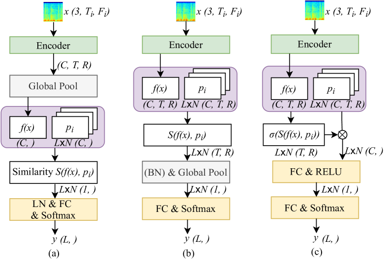
Fig. 1: The frameworks of the prototype learning. (a) Prototype-1D. (b) Prototype-2D with vanilla similarity. (c) Prototype-2D with attention-based similarity. BN = batch normalisation, FC = fully connected layer, LN = layer normalisation, RELU = rectified linear unit. The input $x$ has the dimension of $(3,T_{i},F_{i})$, where $T_{i}$ is the number of time frames and $F_{i}$ is the Mel frequency bins. The other math symbols are corresponding to the definitions in this section.

2.1 Prototype-1D

As the high-level representations include more class-related information than the low-level ones, the prototype layer is trained after a global max pooling layer for 1D prototypes (see Fig. 1(a)). Given an instance $(x,y)$ ($x$: input, $y$: label), the intermediate representation before the prototype layer is denoted by $f(x)$. Through the prototype layer, a set of prototypes $P_{l},l\in[1;L]$ are learnt, where $L$ is the classes’ number. In each $P_{l}$, $p_{i},\ i\in[1;N]$ is a prototype with the same size of $f(x)$, where $N$ is the number of prototypes for each class. The cosine metric is then used to measure the similarities between $f(x)$ and $p_{i}$:

$$S_{1D}(f(x),p_{i})=\frac{f(x)^{T}p_{i}}{\parallel f(x)\parallel_{2}\parallel p_{i}\parallel_{2}}.$$ (1)

The similarity is further fed into a layer normalisation (LN) layer, a fully connected (FC) layer, and a softmax layer for classification. Although the prototype-1D can generate prototypes, it is challenging for 1D prototypes to represent the time and frequency information.

2.2 Prototype-2D

As 2D prototypes can better represent the time-frequency information than 1D prototypes, the prototype layer is placed after the CNN encoder for the similarity measurements (see Fig. 1(b-c)).

Vanilla Similarity. Similar to the prototype-1D learning approach, the calculated similarities are send to the next layers for the classification task (see Fig. 1(b)).

Element-wise Similarity aims to calculate the similarity scores between each pair of time-frequency bins in $(f(x))$ and $p_{i}$. When $f(x)$’s channel number is $C$ and its spatial size is $(T,R)$, the element-wise similarity is calculated by

$$S_{2EV}(f(x),p_{i})=\sum_{c=1}^{C}\frac{f^{c,t,r}(x)p^{c,t,r}_{i}}{\parallel f^{c,t,r}(x)\parallel_{2}\parallel p^{c,t,r}_{i}\parallel_{2}},$$ (2)

where $t\in[1;T]$ and ${r\in[1;R]}$.

Average Similarity is to compute an average score across the similarities between all time-frequency bins of $p_{i}$ and each bin of $f(x)$. Since only part of an audio signal may contain the class-related characteristics, the average similarity is a score between each $f(x)$ bin and $p_{i}$:

$$S_{2AV}(f(x),p_{i})=\mathop{\mbox{avg}}\limits_{t^{\prime}=1,r^{\prime}=1}^{T,R}\sum_{c=1}^{C}\frac{f^{c,t,r}(x)p^{c,t^{\prime},r^{\prime}}_{i}}{\parallel f^{c,t,r}(x)\parallel_{2}\parallel p^{c,t^{\prime},r^{\prime}}_{i}\parallel_{2}}.$$ (3)

Maximum Similarity has the same idea of the average similarity, but select the most similar $p_{i}$ bin for each $f(x)$ bin for structuring the similarity scores at all time-frequency bins. The maximum similarity is computed by

$$S_{2MV}(f(x),p_{i})=\max_{t^{\prime}=1,r^{\prime}=1}^{T,R}\sum_{c=1}^{C}\frac{f^{c,t,r}(x)p^{c,t^{\prime},r^{\prime}}_{i}}{\parallel f^{c,t,r}(x)\parallel_{2}\parallel p^{c,t^{\prime},r^{\prime}}_{i}\parallel_{2}}.$$ (4)

Attention-based Similarity. Apart from the vanilla similarity, the attention-based similarity (see Fig. 1(c)) is employed to learn weighted similarity scores. The calculated similarity scores are processed by a softmax function $\sigma(\cdot)$ for the attention feature maps. As the average similarity is computed as a global score across all $p_{i}$ bins for each $f(x)$ bin, it is not applicable for the attention-based similarity. Therefore, we introduce the element-wise and maximum similarities with the attention mechanism.

Element-wise Similarity is defined by

$$S_{2EA}=\sum_{t=1,r=1}^{T,R}\sigma(S_{2EV}(f(x),p_{i}))f^{c,t,r}(x)p^{c,t,r}_{i}.$$ (5)

Maximum Similarity is calculated at each $(f(x))$ bin $f^{c,t,r}(x)$ and its most similar $p_{i}$ bin $p^{c,t_{max},r_{max}}_{i}$ in Equation (4)

$$S_{2MA}=\sum_{t=1,r=1}^{T,R}\sigma(S_{2MV}(f(x),p_{i}))f^{c,t,r}(x)p^{c,t_{max},r_{max}}_{i}.$$ (6)

2.3 Training

During training the above prototype learning models, the prototypes are learnt as part of the model parameters. The loss function of the neural networks is finally defined by

$$\mathcal{L}=\mathcal{L}_{NLL}+\alpha\mathcal{L}_{dv},$$ (7)

$$\mathcal{L}_{dv}=\frac{\mathop{\mbox{avg}}_{l_{1}=1,l_{2}=1}^{L,L}S_{2AV}(P_{l_{1}},P_{l_{2}})}{\mathop{\mbox{avg}}_{l=1}^{L}S_{2AV}(P_{l},P_{l})},l_{1}\neq l_{2},$$ (8)

where $\mathcal{L}_{NLL}$ is the negative log likelihood (NLL) loss function when the neural networks’ output in Fig. 1 is passed into a logarithm function, $\mathcal{L}_{dv}$ denotes the diverse loss function, and $\alpha$ is a constant value. $\mathcal{L}_{dv}$ aims to reduce the distances among prototypes which represent the same class and increase the distances among prototypes for different classes. The average similarity is experimentally used to evaluate the similarities between each pair of prototypes. In each set of prototypes $P_{l}$ for the class $l$, the similarities of each two different prototypes inside the $P_{l}$ are calculated and averaged, leading to the denominator in Eq. (8); between each two different sets of prototypes $P_{l_{1}}$ and $P_{l_{2}}$, the averaged similarity is also computed as the molecular of Eq. (8).

3 Empirical Evaluation

3.1 Experimental Settings

Data. The Scientific Challenge database released at the International Conference on Biomedical and Health Informatics (ICBHI) 2017 [3] is the largest publicly available collection of audio samples for respiratory sound classification. Totally $920$ audio recordings were collected from seven chest locations (i. e., trachea, anterior left, anterior right, posterior left, posterior right, lateral left, and lateral right) of $126$ participants with four devices (i. e., one microphone and three stethoscopes). The audio recordings have different sampling rates: $4$  kHz, $10$  kHz, and $44.1$ kHz. All recordings derive $6\,898$ respiratory cycles, each of which was annotated with one of the four classes: normal, crackle, wheeze, and both, i. e., crackle $+$ wheeze. The database was split into a training set ($60\,\%$) and a test set ($40\,\%$) for the competition. To optimise the model hyperparameters, we further divide the training set into two subject-independent data sets: a train set ($70\,\%$) and a development set ($30\,\%$) (see Table 1).

Table 1: Distribution of the splitted train/development sets and the official test set in the ICBHI database.

#	Normal	Crackle	Wheeze	Both	$\bm{\sum}$
Train	1 513	616	281	131	2 541
Devel	550	599	220	232	1 601
Test	1 579	649	385	143	2 756
$\bm{\sum}$	3 642	1 864	886	506	6 898

Evaluation Metrics. Although the database contains four labels, it is a common practice to differentiate abnormal cases (crackles, wheezes, and both) and normal cases. Therefore, the following standard benchmarks are used: sensitivity (SE) – equals to the number of true abnormal cases over the total number of abnormal cases, specificity (SP) – the ratio of true normal cases over normal cases, average score (AS) – is the official score of the ICBHI challenge [3] and is the average of SE and SP. Due to class imbalance, we also report the unweighted average recall (UAR) as the generic classification benchmark instead of accuracy [4, 21].

Implementation Details. At the preprocessing stage, all audio recordings are resampled into $4$ kHz due to the various sampling rates of the ICBHI database. A fifth butterworth bandpass filter ($100$ Hz–$1\,800$ Hz) is then applied to exclude noise components, e. g., heart sounds, etc [3]. The respiratory cycles with different durations are unified into audio signals with a fixed time length of $4$ s. On the training stage, $4\,s$ segments are randomly selected from each data sample for improving the flexibility. On the testing stage, the middle $4\,s$ segments are selected to avoid the potential silence at the start and the end. The log Mel spectrograms are further extracted from the audio signals with a window length of $256$, a hop length of $128$, and $128$ Mel bins, as they incorporate several properties of the human auditory system [22].

The CNN encoder is structured by four convolutional blocks with output channel numbers of $64$, $128$, $256$, and $512$, when each convolutional block consists of two covolutional layers with the same output channel number followed by a local max pooling layer with a kernel size of $2\times 2$. For the classification task, the CNN model with a CNN-encoder followed by a global max pooling layer and a FC layer is called ‘CNN-8’.

During training, the CNNs are optimised by an ‘Adam’ optimiser with an initial learning rate of $0.001$ when the batch size is $16$. To stabilise the optmisation, the learning rate is reduced with a factor of $0.9$ at each $200$-th iterations. The training procedure is stopped at the $10\,000$-th iteration. To mitigate the class imbalance problem, each class in $\mathcal{L}_{NLL}$ is given a weight value which is inversely proportional to the samples’ number of the class. The value of $\alpha$ is experimentally set to $0.1$.

Reproducibility Environment. Our experiments are implemented at NVIDIA Geforce GTX 1080 Ti Graphics Cards. The PyTorch code is released at: https://github.com/L3S/PrototypeSound.

3.2 End-to-end Comparison with SOTA Systems

We compare our proposed approach with the following state-of-the-art (SOTA) methods on the ICBHI database. (1) MFCC-HG [23]: The Mel-frequency cepstral coefficients (MFCCs) are extracted with their first derivatives as the input of the classifiers, which were structured with hidden Markov models and Gaussian mixture models. (2) MFCC-BDT [24]: The MFCCs are fed into a boosted decision tree with four leaves for four classes. (3) STFT-WS [25]: The frequency features integrated from the short-time Fourier transform (STFT) spectrograms and the statistical & spectral features from the wavelet coefficients were classified by support vector machines. (4) STFT-WB [26]: The STFT spectrograms and wavelet scalograms were processed by a bi-ResNet model. (5) STFT-RSESA [6]: The STFT spectrograms were fed into a ResNet model with a squeeze-and-excitation block and a spatial attention block. Table 2 presents the result. Our approach performs better than all of the SOTA methods when comparing the AS scores. Our approach significantly outperforms the MFCC-HG approach ($p<.001$ in a one-tailed z-test).

Table 2: Classification performance [%] compared with the SOTA approaches on the test set.

	SE	SP	AS	UAR
MFCC-HG [23]	–	–	39.56	–
MFCC-BDT [24]	20.81	78.05	49.43	–
STFT-WS [25]	–	–	49.86	–
STFT-WB [26]	31.12	69.20	50.16	–
STFT-RSESA [6]	17.84	81.25	49.55	–
Ours	27.78	72.96	50.37	36.16

3.3 Ablation Study

Table 3 shows our ablation study on the prototype layers and batch normalisation in the prototype-2D with the vanilla similarities. In general, the performance of most prototype learning variants is comparable to that of the basic CNN-8 model. Particularly, the UAR values are increased by several variants learnt by prototype learning, leading to higher SE values on the abnormal classes (crackle, wheeze, and both). Both high accuracy and interpretability are reserved in our approach.

Table 3: Ablation study on the prototype layers and the batch normalisation (BN) when $N=1$. Pt = Prototype.

Performance [%]	Devel	Test
Variants	AS	SE	SP	AS	UAR
CNN-8	52.99	39.42	59.72	49.57	40.36
Pt-1D	51.44	46.73	45.85	46.29	43.34
Pt-2D-EleSim-Van w/o BN	47.44	48.68	41.10	44.89	40.39
Pt-2D-EleSim-Van w/ BN	52.22	27.78	72.96	50.37	36.16
Pt-2D-EleSim-Attention	48.36	46.22	37.62	41.92	40.06
Pt-2D-AvgSim-Van w/o BN	33.42	53.36	39.27	46.31	38.82
Pt-2D-AvgSim-Van w/ BN	55.43	44.94	55.41	50.18	43.76
Pt-2D-MaxSim-Van w/o BN	42.94	50.47	39.52	44.99	40.80
Pt-2D-MaxSim-Van w/ BN	11.85	61.94	00.00	30.97	35.36
Pt-2D-MaxSim-Attention	50.81	49.96	37.62	43.79	43.50

The batch normalisation procedure is also analysed in our models with the vanilla similarities. In Table 3, batch normalisation leads to improvements for the vanilla element-wise similarity and the vanilla average similarity, which it results in very low performance (i. e., $\mbox{SP}=0$) for the vanilla maximum similarity. In this regard, we select the best batch normalisation setting for each vanilla similarity for further experiments.

3.4 Sensitivity Analysis

Number of Prototypes. We compare the effect of prototype numbers for each approach in Fig. 2. The performances of the proposed models are comparable when $N$ varies from $1$ to $5$, indicating generating one prototype per class is sufficient.

Similarity Comparison. Prototype-2D with vanilla element-wise similarity mostly perform better than the other other approaches, perhaps due to its capability of generating prototypes with time-frequency information and less parameters than the models with the attention-based similarity. When comparing the three vanilla similarities, the vanilla element-wise similarity always outperforms the other two.

Fig. 2: Performance [$\%$] comparison on the test set among different prototype learning approaches with a given number of prototypes per class. The green bars represent the UAR values, and the occluded white bars show the AS scores.

3.5 Projection of Prototypes

As the generated prototypes contain multiple channels and have a small spatial size due to local pooling layers, it is challenging to visualize the prototypes. Hence, we project the prototypes to their closest inputs of the models by searching for the closest intermediate representation $f(x)$:

$$\min dist_{j=1}^{J}(p_{i},f(X_{j})),\ dist(p_{i},f(X_{j}))=e^{(-S)},$$ (9)

where $X$ means all $J$ instances, $j$ is the index number. $dist$ is the distance, and $S$ denotes the similarity. Herein, the log Mel spectrograms calculated by the projection procedure for our best model on the test set are depicted in Fig. 3. The projection of prototypes is helpful to analyse the characteristics of each class of respiratory sounds. We can see that, the normal respiratory cycles are regular, while the others are not. As crackle sounds are attributed to sudden bursts of air within bronchioles, therefore they are explosive and transient, and non-musical [27]. The example of Fig. 3(b) can represent the above character of crackle sounds. Different from crackle sounds, wheeze sounds are continuous and commonly observed in patients with obstructive airways diseases, e. g., asthma (AS) and chronic obstructive pulmonarydisease (COPD) [28]. Musical wheeze sounds are sinusoidal sounds in time domain and are superimposed on normal breath sounds [28]. In Fig. 3(c), the regularity of the sounds can reflect the nature of wheeze sounds. The wheeze log Mel spectrogram has smaller coefficients on a range of Mel frequencies than the crackle one, probably indicating the wheeze sound is weaker. In Fig. 3(d), the musicality of wheeze sound is difficult to be observed when wheeze and crackle sounds occur simultaneously.

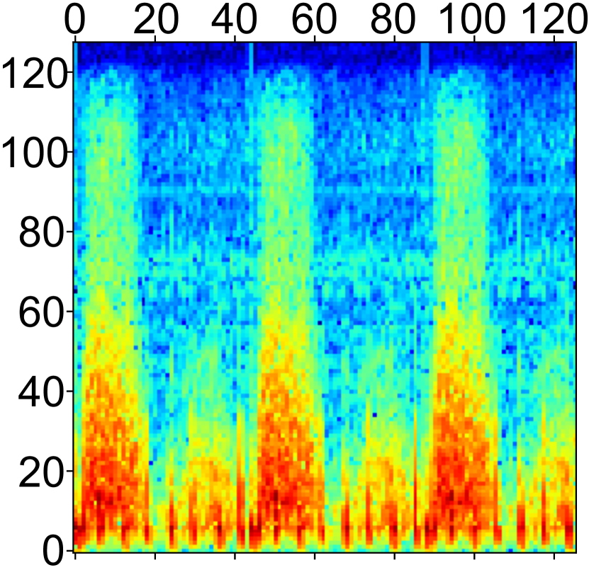
(a) Normal

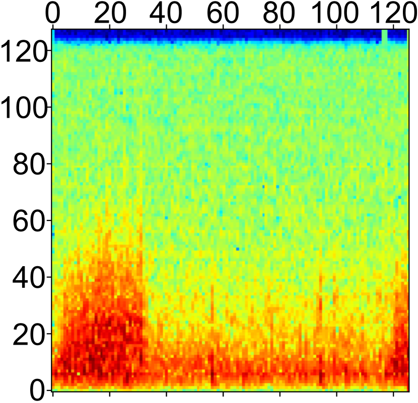
(b) Crackle

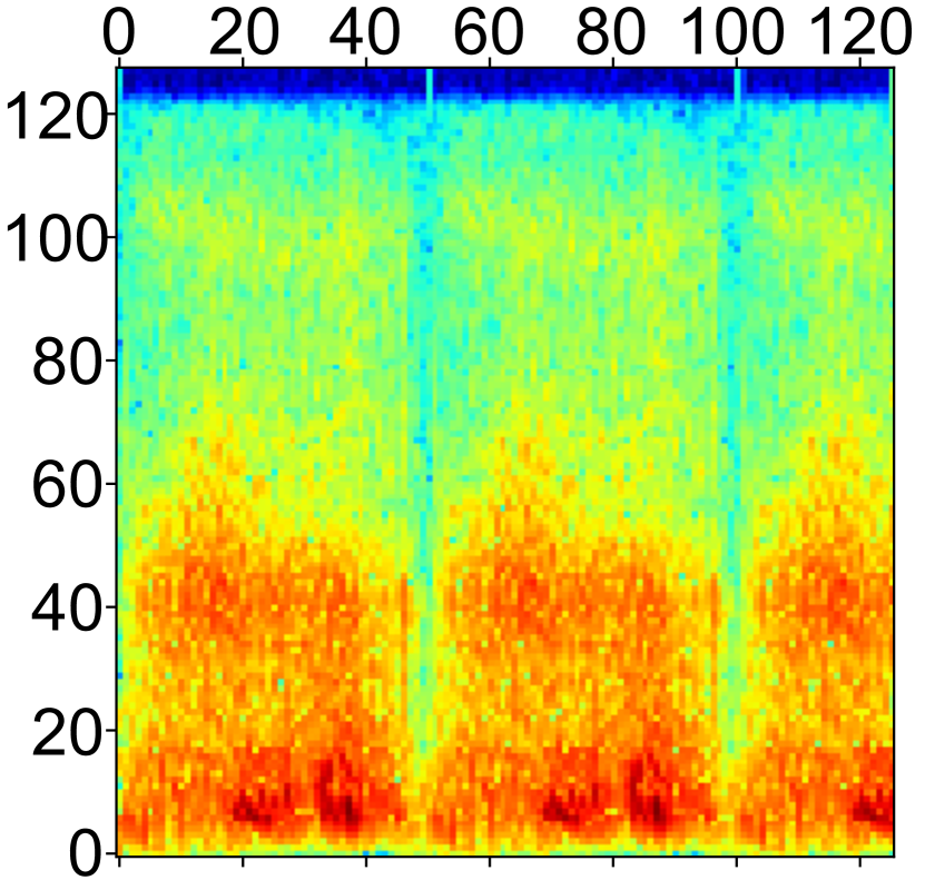
(c) Wheeze

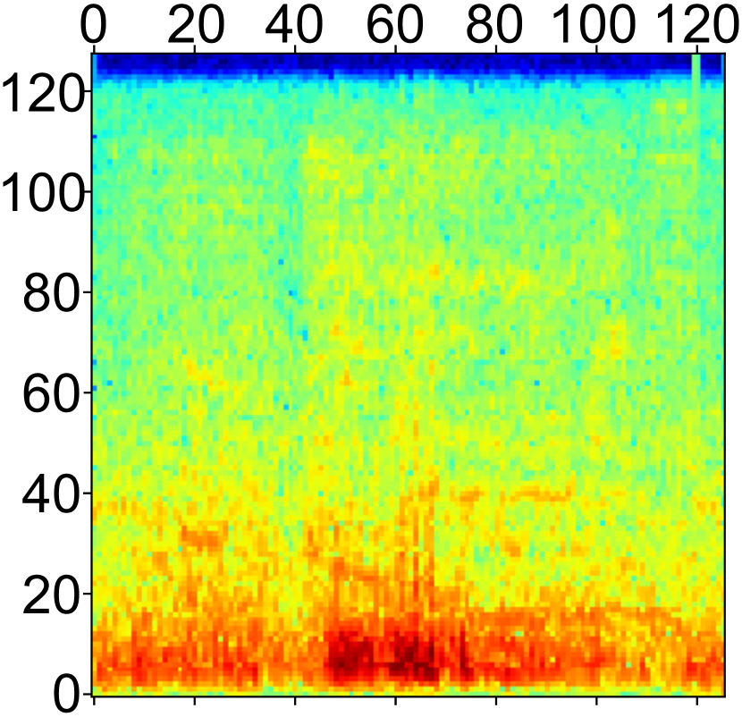
(d) Both

Fig. 3: The closest log Mel spectrograms to the prototypes. The X-axis is time frame and the Y-axis is Mel frequency.

4 Conclusion

Prototype learning paradigm, which is widely used for example-based explanation or case-based reasoning, recently has been transplanted to classification for jointly improving the classification performance and the result interpretability. This paper developed a prototype learning framework for interpretable respiratory sound classification by generating prototypical feature maps that were integrated into the training of the predictive model. Not only increasing the predictivity, the learnt prototypes can introduce new cases to assist physicians in learning from automatic diagnosis and making informed decisions. In future work, we plan to explore other types of explanations such as concepts and criticisms [14] as well as reconstruct the original audio signals.

Acknowledgments. This research was funded by the Federal Ministry of Education and Research (BMBF), Germany under the project LeibnizKILabor with grant No. 01DD20003.

References

- [1] R. Pramono, S. Bowyer, and E. Rodriguez-Villegas, “Automatic adventitious respiratory sound analysis: A systematic review,” PLOS ONE, vol. 12, no. 5, pp. e0177926, 2017.
- [2] S. Tabatabaei et al., “Methods for adventitious respiratory sound analyzing applications based on smartphones: A survey,” IEEE Rev Biomed Eng, vol. 14, pp. 98–115, 2020.
- [3] B. Rocha et al., “An open access database for the evaluation of respiratory sound classification algorithms,” Physiol. Meas., vol. 40, no. 3, 2019.
- [4] W. Song, J. Han, and H. Song, “Contrastive embeddind learning method for respiratory sound classification,” in Proc. ICASSP, Virtual, 2021, pp. 1275–1279.
- [5] Y. Chang, Z. Ren, and B. Schuller, “Transformer-based CNNs: Mining temporal context information for multi-sound COVID-19 diagnosis,” in Proc. EMBC, Virtual, 2021, pp. 2335–2338.
- [6] Z. Yang et al., “Adventitious respiratory classification using attentive residual neural networks,” in Proc. INTERSPEECH, Virtual, 2020, pp. 2912–2916.
- [7] P. Chong, N.-M. Cheung, Y. Elovici, and A. Binder, “Towards scalable and unified example-based explanation and outlier detection,” IEEE Trans Image Process, vol. 31, pp. 525 – 540, 2020.
- [8] C. Chen et al., “This looks like that: Deep learning for interpretable image recognition,” in Proc. NIPS, Vancouver, Canada, 2019, pp. 1–12.
- [9] O. Li, H. Liu, C. Chen, and C. Rudin, “Deep learning for case-based reasoning through prototypes: A neural network that explains its predictions,” in Proc. AAAI, New Orleans, LA, 2018, pp. 3530–3537.
- [10] D. Rymarczyk, L. Struski, J. Tabor, and B. Zieliński, “ProtoPShare: Prototypical parts sharing for similarity discovery in interpretable image classification,” in Proc. KDD, Virtual, 2021, pp. 1420–1430.
- [11] S. Arık and T. Pfister, “ProtoAttend: Attention-based prototypical learning,” J. Mach. Learn. Res., vol. 21, pp. 1–35, 2020.
- [12] Y. Ming, P. Xu, H. Qu, and L. Ren, “Interpretable and steerable sequence learning via prototypes,” in Proc. KDD, Anchorage, AK, 2019, pp. 903–913.
- [13] M. Nauta, R. van Bree, and C. Seifert, “Neural prototype trees for interpretable fine-grained image recognition,” in Proc. CVPR, Virtual, 2021, pp. 14933–14943.
- [14] P. Zinemanas et al., “An interpretable deep learning model for automatic sound classification,” Electronics, vol. 10, no. 7, pp. 850, 2021.
- [15] T. Yan et al., “Coughing-based recognition of Covid-19 with spatial attentive ConvLSTM recurrent neural networks,” in Proc. INTERSPEECH, Brno, Czechia, 2021, pp. 4154–4158.
- [16] A. Coluccia, A. Fascista, and G. Ricci, “Robust CFAR radar detection using a k-nearest neighbors rule,” in Proc. ICASSP, Virtual, 2020, pp. 4692–4696.
- [17] Z. Ren, Q. Kong, J. Han, M. Plumbley, and B. Schuller, “CAA-Net: Conditional atrous CNNs with attention for explainable device-robust acoustic scene classification,” IEEE Trans Multimedia, vol. 23, pp. 4131–4142, 2020.
- [18] M. Sudhakar et al., “Ada-sise: Adaptive semantic input sampling for efficient explanation of convolutional neural networks,” in Proc. ICASSP, Virtual, 2021, pp. 1715–1719.
- [19] P. Hase, C. Chen, O. Li, and C. Rudin, “Interpretable image recognition with hierarchical prototypes,” in Proc. HCOMP, Palo Alto, CA, 2019, pp. 32–40.
- [20] Y. Chang, X. Jing, Z. Ren, and B. Schuller, “CovNet: A transfer learning framework for automatic COVID-19 detection from crowd-sourced cough sounds,” Frontiers in Digital Health, vol. 3, no. 799067, pp. 1–11, 2022.
- [21] Z. Ren, A. Baird, J. Han, Z. Zhang, and B. Schuller, “Generating and protecting against adversarial attacks for deep speech-based emotion recognition models,” in Proc. ICASSP, Virtual, 2020, pp. 7184–7188.
- [22] A. Martinez, N. Moritz, and B. Meyer, “Should deep neural nets have ears? The role of auditory features in deep learning approaches,” in Proc. INTERSPEECH, Singapore, 2014, pp. 2435–2439.
- [23] N. Jakovljević and T. Lončar-Turukalo, “Hidden markov model based respiratory sound classification,” in Proc. ICBHI, Thessaloniki, Greece, 2017, pp. 39–43.
- [24] G. Chambres, P. Hanna, and M. Desainte-Catherine, “Automatic detection of patient with respiratory diseases using lung sound analysis,” in Proc. CBMI, La Rochelle, France, 2018, pp. 1–6.
- [25] G. Serbes, S. Ulukaya, and Y. Kahya, “An automated lung sound preprocessing and classification system based onspectral analysis methods,” in Proc. ICBHI, Thessaloniki, Greece, 2017, pp. 45–49.
- [26] Y. Ma et al., “LungBRN: A smart digital stethoscope for detecting respiratory disease using bi-ResNet deep learning algorithm,” in Proc. BioCAS, Nara, Japan, 2019, pp. 1–4.
- [27] Gorkem Serbes, C Okan Sakar, Yasemin P Kahya, and Nizamettin Aydin, “Feature extraction using time-frequency/scale analysis and ensemble of feature sets for crackle detection,” in EMBS, 2011, pp. 3314–3317.
- [28] Styliani A Taplidou and Leontios J Hadjileontiadis, “Wheeze detection based on time-frequency analysis of breath sounds,” Computers in Biology and Medicine, vol. 37, no. 8, pp. 1073–1083, 2007.