Range and Bearing Data Fusion for Precise Convex Network Localization

Abstract

Hybrid localization in GNSS-challenged environments using measured ranges and angles is becoming increasingly popular, in particular with the advent of multimodal communication systems. Here, we address the hybrid network localization problem using ranges and bearings to jointly determine the positions of a number of agents through a single maximum-likelihood (ML) optimization problem that seamlessly fuses all the available pairwise range and angle measurements. We propose a tight convex surrogate to the ML estimator, we examine practical measures for the accuracy of the relaxation, and we comprehensively characterize its behavior in simulation. We found that our relaxation outperforms a state of the art SDP relaxation by one order of magnitude in terms of localization error, and is amenable to much more lightweight solution algorithms.

I Introduction

Spatial awareness is a hallmark of contemporary real-world systems and applications, particularly when multiple agents collaborate to attain common goals. Location technologies are key for operation in GNSS-challenged environments, like underwater [1] or indoor [2] and city skyscraper areas [3], and also in many applications in wireless communications [4], sensor networks [5], IoT [6], medicine [7, 8], etc. Our work addresses the network localization problem [9], where multiple networked agents cooperate in sensing and computation to jointly estimate their unknown positions.

Related work

There is a vast literature for range-based network localization, from multidimensional scaling[10, 11] to nonconvex ML estimation [12, 13], convexifications of ML problems [14, 15, 16], and other convex heuristics to match measured data to a data model [17, 18].

Several current technologies not only give access to accurate distance measurements, but also provide angle information. These added measurements can improve the quality of estimates or reduce the amount of resources spent to obtain a reasonable localization precision. 5G is an especially noteworthy example where the value of hybrid measurements has been noted [19, 4], and information-theoretic bounds are available to characterize their impact [20, 5]. While the topic of single-source range/bearing localization is reasonably well covered in the technical literature, specific references addressing network localization algorithms for that data model are surprisingly scarce [21, 22, 23, 24, 25, 26] (see also the recent survey [5]). Yet, the potential usefulness of such algorithms, e.g., in massive MIMO communication scenarios seems quite obvious. Below, we focus our literature review on the subclass of hybrid network localization algorithms derived from single convex formulations, which avoid initialization issues affecting other types of approaches. The importance of considering hybrid measurements was emphasized early on in [21], but a clear statement of the graphical conditions for localizability of the network assuming range and bearing measurements was only formalized in [23]. One of the first convex formulations was a semidefinite program (SDP) proposed in [22] for 2D scenarios. Angle constraints were manipulated into a form similar to the one used for ranges, and incorporated into an existing range-only SDP. Reference [27] addresses the single-source and network localization problems through a convex relaxation of a nonconvex least-squares cost function, and [25] extends this to mobile setups. The very recent work in [28] explores the problem using belief propagation, but relies on linearized approximations. Recently, [26] takes the ML estimator for the original static scenario and considers Gaussian noise for ranges and von Mises–Fisher noise for bearings. This very interesting work performs several approximations and formulates the problem as an SDP. However, the manipulations involve squaring of range and angular terms, which is known to amplify noise and degrade localization accuracy [29, 30].

Another important line of work for hybrid network localization, particularly in the scope of wireless communications, uses RSS-based measurements as proxies for ranges (see [31, 32] for an extensive list of references). The model for RSS measurements is quite different from the one that we adopt for ranges, and so are the manipulations and relaxations used in localization algorithms.

Contributions

As in [26] we adopt a ML approach assuming Gaussian noise for range measurements and von Mises–Fisher noise for bearings, leading to a difficult to solve nonconvex problem. Unlike [26] we do not approximate the problem via squaring of range or angle terms, but instead adopt an unconventional relaxation technique that in our simulations attains one order of magnitude more accurate results. The approach works in 2D and 3D (or in any ambient dimension). As a second contribution, we provide certificates of optimality that indicate if the minimizer of the convex surrogate coincides with that of the nonconvex ML estimator. While our formulation is amenable to parallelization, the derivation of tailored solution algorithms is beyond the scope of this paper. Our main goal here is to highlight and characterize the excellent accuracy of the proposed approximate ML relaxation.

II Problem statement

We model the network of agents as a graph ${\mathcal{G}}=({\cal V},{\cal E})$ where ${\cal V}=\{1,\cdots,n\}$ denotes the set of $n$ agents with unknown positions, and each edge $i\sim j\in{\cal E}$ indicates that agents $i$ and $j$ can communicate, and can measure a noisy version of their scalar distance $d_{ij}$, that we consider symmetrical. We express the position of agent $i$ in the ambient space as $x_{i}\in\mathbb{R}^{p}$, where $p\in\{2,3\}$ in practical applications. We also define an edge set ${\cal E}_{u}\in{\cal E}$ as the set of edges providing noisy angle measurements between agents. Bearing data is measured as a unit vector $u_{ij}$ expressed in the world frame. For localization in a global reference frame, the problem assumes the existence of a set ${\cal A}$ of landmarks or anchors whose absolute positions $\{a_{k}\}_{k\in{\cal A}}$ are known. Each agent $i$ can measure noisy ranges $\{r_{ik}\}$ for all $k\in{\cal A}_{i}\subseteq{\cal A}$ and, possibly, bearings $\{v_{ik}\}_{k\in{\cal U}_{i}}$, where ${\cal U}_{i}\subseteq{\cal A}_{i}$ is the subset of anchors reachable from node $i$ that also provide bearing measurements. We note that these assumptions differ from those of [31], e.g., where every range-like (RSS) measurement needs a matching angular measurement. In some settings ranging devices are much cheaper than those used to measure angles[1], so requiring the latter only in a subset of nodes may be desirable.

Noise model

We model noisy range measurements $d_{ij}$, $r_{ik}$ as independent and identically distributed (iid) normal random variables centered at the true ranges with standard deviations $\sigma_{ij}$ and $\varsigma_{ik}$, respectively. Similarly, we model noisy bearings as iid von Mises-Fisher random variables, independent from ranges, centered at the true bearings with concentration parameters $\kappa_{ij}$, $\varkappa_{ik}$. In the following section we formulate the ML estimator for the positions of all the agents $x=\{x_{i}\}_{i=1}^{n}$ as a nonconvex optimization problem.

Maximum likelihood localization with distance and angle measurements

Assuming the noise models discussed above, we can write the maximum likelihood estimator for the positions $x$ of the overall network as

$$\operatornamewithlimits{minimize}_{x}\;f(x)+f_{u}(x),$$ (1)

where $f$ represents the range-related terms, and $f_{u}$ represents the bearing terms. Specifically, we have, as $f(x)$,

$$\sum_{i\sim j\in{\cal E}}\frac{1}{\sigma_{ij}^{2}}(\|x_{i}-x_{j}\|-d_{ij})^{2}+\sum_{i}\sum_{k\in{\cal A}_{i}}\frac{1}{\varsigma_{ik}^{2}}(\|x_{i}-a_{k}\|-r_{ik})^{2},$$ (2)

and, for the bearings, $f_{u}(x)$ is defined as

$$\sum_{i\sim j\in{\cal E}_{u}}\left(\kappa_{ij}u_{ij}^{T}\frac{x_{i}-x_{j}}{\|x_{i}-x_{j}\|}\right)+\sum_{i}\sum_{k\in{\cal U}_{i}}\left(\varkappa_{ik}v_{ik}^{T}\frac{x_{i}-a_{k}}{\|x_{i}-a_{k}\|}\right).$$ (3)

The unconstrained problem (1) is nonconvex due to both terms (2), (3) and difficult to solve globally. Function $f$ in (2) is nonconvex because the argument of the square has a negative region when $\|x_{i}-x_{j}\|<d_{ij}$ (the same for the anchor terms). Non-convexity of $f_{u}$ stems from $x_{i}-x_{j}$ appearing nonlinearly in the denominator. We will overcome this difficulty by relaxing the problem to a convex one, as presented in the next section. Later, we will see in numerical results that the relaxation retains good estimation accuracy.

III Convex relaxation

Following [15], we rewrite each term in (2) as

$$(\|x_{i}-x_{j}\|-d_{ij})^{2}=\min_{\|y_{ij}\|=d_{ij}}\|x_{i}-x_{j}-y_{ij}\|^{2},$$ (4)

where the constraint set represents a sphere centered at the origin with radius $d_{ij}$. When $y_{ij}$ is placed optimally on the circle with radius $d_{ij}$ its distance to $x_{i}$ is $\lvert\|x_{i}-x_{j}\|-d_{ij}\rvert$, as intended. The auxiliary variable is readily worked out in closed form as $y_{ij}=d_{ij}\frac{x_{i}-x_{j}}{\|x_{i}-x_{j}\|}$. Focusing on inter-node terms only for clarity, we have for the hybrid ML problem

$$\begin{split}p_{1}=&\min_{x,y}\sum_{i\sim j}\|x_{i}-x_{j}-y_{ij}\|^{2}-\kappa_{ij}{u}_{ij}^{T}\frac{x_{i}-x_{j}}{\|x_{i}-x_{j}\|}\\ &\operatornamewithlimits{\text{subject to}}\>\|y_{ij}\|=d_{ij},\end{split}$$ (5)

where $y$ is the concatenation of $\{y_{ij},i\sim j\}$, constraints are on all edges of ${\cal G}$, and $p_{1}$ denotes the optimal value of the nonconvex problem (1). This can be equivalently written as

$$\begin{split}p_{1}=&\min_{x,y}\sum_{i\sim j}\|x_{i}-x_{j}-y_{ij}\|^{2}-\frac{\kappa_{ij}}{d_{ij}}u_{ij}^{T}y_{ij}\\ &\operatornamewithlimits{\text{subject to}}\>\|y_{ij}\|=d_{ij},\>y_{ij}=d_{ij}\frac{x_{i}-x_{j}}{\|x_{i}-x_{j}\|},\end{split}$$ (6)

Note that the first constraint is redundant given the second one. We will now relax our problem by dropping the second constraint in (6), obtaining

$$\begin{split}p_{2}=&\min_{x,y}\sum_{i\sim j}\|x_{i}-x_{j}-y_{ij}\|^{2}-\tilde{u}_{ij}^{T}y_{ij}\\ &\operatornamewithlimits{\text{subject to}}\>\|y_{ij}\|=d_{ij},\end{split}$$ (7)

where $\tilde{u}_{ij}=\frac{\kappa_{ij}}{d_{ij}}u_{ij}$. As the constraint set was enlarged, we have $p_{2}\leq p_{1}$.

Disk relaxation

Now we relax the constraint set from the sphere to the ball $\{y\colon\|y\|\leq d_{ij}\}$, its convex hull, to obtain an approximation of the variational representation for range terms (4)

$$\min_{\|y_{ij}\|\leq d_{ij}}\|x_{i}-x_{j}-y_{ij}\|^{2}.$$ (8)

As discussed in [15], replacing the terms (4) in the range-only cost function (2) with the modified ones (8) is beneficial for outlier rejection; if $y_{ij}$ can be placed anywhere on the ball, not just on the border, this will limit the contribution of large disks created by outliers with large values of $d_{ij}$. However, placing $x_{i}$ and $y_{ij}$, $y_{il}$ anywhere inside the intersection area of such disks will yield zero contribution to the cost.

Now consider the hybrid problem (7) after the same disk relaxation of its constraint sets (relaxing $\|y_{ij}\|=d_{ij}$ to $\|y_{ij}\|\leq d_{ij}$). The newly added angular terms will break the flatness of range contributions discussed previously, biasing the $y$ variables back towards the borders of the disks along the directions measured. Effectively, this formulation approximates the intended behavior of the original one in (6) with equality constraints, while doing so in a soft way that preserves the ability to seamlessly reduce the impact of outliers in range measurements. The complete relaxed ML problem is as follows

$$\begin{split}\operatornamewithlimits{minimize}_{x,y,w}&\sum_{i\sim j}\|x_{i}-x_{j}-y_{ij}\|^{2}-\tilde{u}_{ij}^{T}y_{ij}\\ &+\sum_{i\in{\cal V},k\in{\cal A}_{i}}\|x_{i}-a_{k}-w_{ik}\|^{2}-\tilde{v}_{ij}^{T}w_{ik}\\ \operatornamewithlimits{\text{subject to}}&\>\|y_{ij}\|\leq d_{ij},\>\|w_{ik}\|\leq r_{ik},\end{split}$$ (9)

where $w_{ik}$ have the corresponding role to $y_{ij}$ regarding anchor-node terms, and $\tilde{v}_{ik}=\frac{\varkappa_{ik}}{r_{ik}}v_{ik}$. This non-standard relaxation is the main contribution of this work.

IV Suboptimality analysis

After presenting a convex relaxation to the nonconvex problem (1) we now perform a tightness analysis. From the derivation of our relaxation we know that if the optimal edge variables $y_{ij}^{\star}$, anchor-node variables $w_{ik}^{\star}$, and node positions $x_{i}^{\star}$ obey the dropped equality constraints $y_{ij}^{\star}=d_{ij}\frac{x_{i}^{\star}-x_{j}^{\star}}{\|x_{i}^{\star}-x_{j}^{\star}\|},\qquad w_{ik}^{\star}=r_{ik}\frac{x_{i}^{\star}-a_{k}}{\|x_{i}^{\star}-a_{k}\|},$ then the solution $(x^{\star},y^{\star},w^{\star})$ of problem (9) is also the solution of the original nonconvex problem (6), considering anchors. We measure the suboptimality in the optimization variables by the average $p_{1}$-residual

$$E_{1}=\frac{1}{|{\cal E}|}\sum_{i\sim j}\left\|y_{ij}^{\star}-d_{ij}\frac{x_{i}^{\star}-x_{j}^{\star}}{\|x_{i}^{\star}-x_{j}^{\star}\|}\right\|\\ +\sum_{i\in{\cal V},k\in{\cal A}_{i}}\frac{1}{|{\cal A}_{i}|}\left\|w_{ik}^{\star}-r_{ik}\frac{x_{i}^{\star}-a_{k}}{\|x_{i}^{\star}-a_{k}\|}\right\|.$$ (10)

A weaker, but rather useful result, is the verification of $\|y_{ij}\|=d_{ij}$ and $\|w_{ik}\|=r_{ik},$ and the computation of the average $p_{2}$-residual

$$E_{2}=\frac{1}{|{\cal E}|}\sum_{i\sim j}|\|y^{\star}_{ij}\|-d_{ij}|+\sum_{i\in{\cal V},k\in{\cal A}_{i}}\frac{1}{|{\cal A}_{i}|}|\|w^{\star}_{ik}\|-r_{ik}|.$$ (11)

Both results are important to understand how good our estimate for the node positions $x$ is. We point out that, in the presence of noisy measurements, $E_{1}$ will not be zero, but in our simulations $E_{2}$ is indeed very close to zero. As the value of $E_{2}$ is consistently very small in our numerical experiments, the norms of edge variables $y_{ij}$ and anchor-node variables $w_{ik}$ effectively equal the measured ranges. Thus, it is also useful to consider the suboptimality angles defined by

$$\theta_{ij}=\arccos\left\langle\frac{y_{ij}^{\star}}{\|y_{ij}^{\star}\|},\frac{x_{i}^{\star}-x_{j}^{\star}}{\|x_{i}^{\star}-x_{j}^{\star}\|}\right\rangle,$$ (12)

where $\langle\cdot,\cdot\rangle$ denotes the usual inner product of two (unit-norm) vectors. We also define $\beta_{ik}$ similarly to $\theta_{ij}$, but with node-anchor variables. Jointly with $E_{2}$, these angles show how much our estimates deviate from optimality.

V Numerical experiments

To analyse performance and suboptimality, we randomly generated geometric networks based on sensing ranges, and tested each network for range localizability [33], to ascertain that there is no ambiguity in the solution space inherent to network configurations. In the interest of visualization, we chose a 2D environment to perform our experiments. We stress, however, that our algorithm is agnostic to the dimensionality of the ambient space.

Problem size

We test our method on networks with $n=100$, and networks of $n=10$ nodes. The smaller sized networks are used for comparison with a state-of-the-art SDP relaxation. Larger networks could not be solved with a generic SDP solver. Agents and anchors are randomly located in a $7\times 7\>m^{2}$ region, and, following the minimum number of anchors allowed for range-only localization in 2D, we set $|{\cal A}|=3$. We emphasize that our method, minimizing a quadratic over a convex set, practically can accommodate much larger problem sizes than SDP-based formulations.

Measurement data generation

Range measurements are contaminated by noise with standard deviation of 0.5 m, while bearing measurements are corrupted by noise with standard deviation of $2^{\circ}$. The concentration parameter associated with each angular measurement is the inverse of the variance in radians. These uncertainty values were drawn from [1], regarding a relevant application of hybrid localization algorithms: the underwater scenario.

Simulation parameters

The number of Monte Carlo (MC) trials, $M$, in each experiment, was obtained by instantiating problems, running estimators, computing metrics, and stopping whenever the running averages across MC trials $\langle H\rangle_{M}=\frac{1}{M}\sum_{m=1}^{M}H_{m}$ were sufficiently stable. Here, $H$ stands for an error, for example, $E_{1}$ in (10), $E_{2}$ in (11) or the angles $\theta_{ij}$ and $\beta_{ik}$ in (12), computed from data of MC trial $m$.

Tightness measures

We first check in simulation that the convex relaxation (9) is tight regarding the nonconvex problem (7). For this experiment, the number of MC trials was 209.

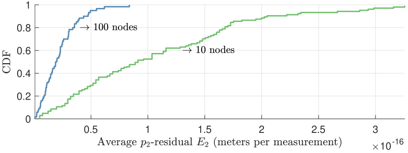
Figure 1: The empirical CDF shows that, for all MC trials, average $p_{2}$-residuals $E_{2}$ are below $10^{-15}$. Thus, for all our experiments, $\|y_{ij}^{\star}\|=d_{ij}$, and $\|w_{ik}^{\star}\|=r_{ik}$ so, for all practical purposes, there is no suboptimality gap by approximating the nonconvex problem (7) with the convex relaxation (9). We also observe that scaling the problem from 10 to 100 nodes slightly increases performance. In fact, due to having a denser network and more measurements — albeit with more unknowns — our estimator shows less violation of the nonconvex ML constraint dropped in (9).

The empirical Cumulative Distribution Function (CDF) of the  $E_{2}$ residuals in Fig. 1 evidences that, for all MC trials, the relaxation of the equality constraint on the edge and node-anchor variables is tight, and that the solution of (9) practically coincides with the solution of (7). This is a very interesting result reinforcing the intuitive idea that if we add new independent measurements we achieve better estimation. Now we investigate $p_{1}$-residuals, associated with dropping the constraints $y_{ij}=d_{ij}\frac{x_{i}-x_{j}}{\|x_{i}-x_{j}\|}$ and $w_{ik}=r_{ik}\frac{x_{i}-a_{k}}{\|x_{i}-a_{k}\|}.$

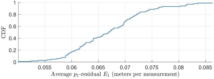
Figure 2: Empirical CDF for the average $p_{1}$-residual for networks with 10 nodes. Approximating the nonconvex problem (6) with the nonconvex relaxation (7) represents an average error per measurement below 9 cm.

Fig. 2 shows that the $p_{1}$-residual $E_{1}$ is smaller than range noise.

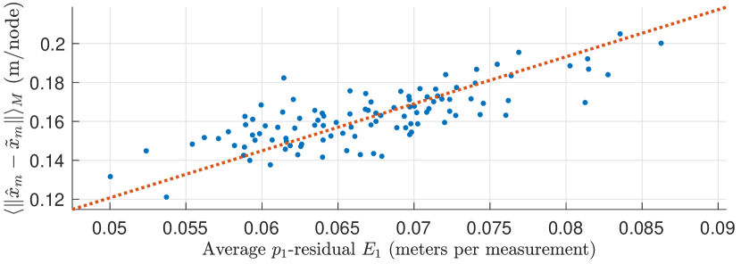
Figure 3: There is a strong correlation between the $E_{1}$ residual error and position error. In MC trial $m$, we compute the error of our estimate $\hat{x}_{m}$ to the numerical minimizer of the nonconvex original problem (1), $\tilde{x}_{m}$ when initialized on the ground truth pre-noise node positions.

The approximation error $E_{1}$ grows linearly with the error in the estimates, as seen in Fig. 3. In fact, when plotted against the average error over MC trials between our estimate $\hat{x}_{m}$, and the numerical minimizer $\tilde{x}_{m}$ of (1) initialized with the true positions before noise addition, we see that the two errors are highly correlated. As we have seen in Fig. 1, there is negligible error associated with the last relaxation. Whenever this is true, it is more illuminating to observe the approximation error in terms of the suboptimality angles $\theta_{ij}$ (12) and $\beta_{ik}$.

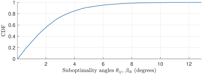
Figure 4: Empirical CDF for suboptimality angles (12). Angles are small. We observe that more than 80% of the errors are below 4^∘. We can, then, conclude that the relaxation gives quite accurate results. The CDF shows more points than the previous figures because all angles are shown (they are not averaged).

Fig. 4 evidences that the relaxation from problem (6) to (7) does not incur a large approximation error. We stress that the suboptimality angles in (12), jointly with the verification that $E_{1}$ is virtually zero, are intuitive metrics of how far is the optimum of the true ML estimator for hybrid localization.

Benchmark

So far we have studied the performance of our relaxation with respect to the nonconvex ML estimator, using our measures of suboptimality in the solution. This section presents a comparison with a state of the art method [26], using precisely the same data model as our proposal. We used the generic solver CVX [34] to obtain the SDP estimate.

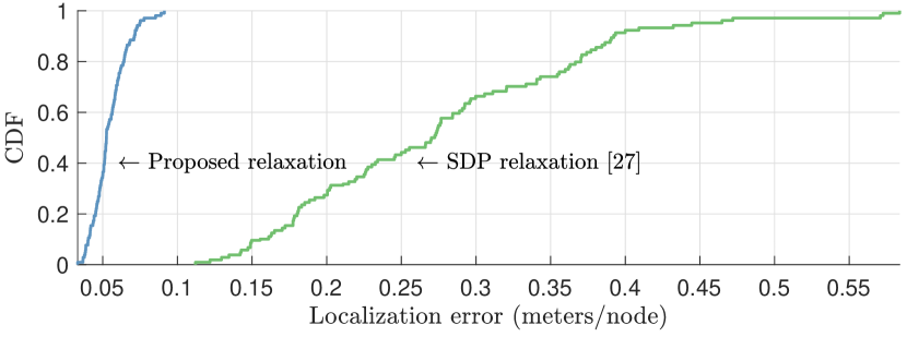
Figure 5: Empirical CDF of localization error for the proposed relaxation, compared with the SDP relaxation [26]. Not only does our relaxation fare better in minimum, average, and maximum error per node, but the slope of the error CDF is also much steeper. This indicates low variance in the estimator performance. The median is one order of magnitude smaller for the proposed relaxation, and the maximum localization error is below 0.1 m, while the SDP method can surpass 0.55 m of localization error per node.

This time we will measure performance based on the average localization error defined as $e=\frac{1}{n}\sum_{i}\|\hat{x}_{i}-x_{i}^{\star}\|$, where $\hat{x}_{i}$ is the optimum of the position of node $i$, given by one of the relaxations, and $x_{i}^{\star}$ is the true position, before measurement noise. Fig. 5 evidences the accuracy gain in using the proposed approach. In our experiments, our approach always yielded less than 0.1 m in localization error, while the SDP relaxation resulted in a spreaded error from 0.1 m to 0.55 m. Summing up, with one order of magnitude smaller error, our relaxation has less variance and lower computational demands, offering even a practical metric of suboptimality for our estimates.

Scalability

Next, we ran 120 MC trials with similar random geometric networks, but now with 100 nodes. We could not run the SDP relaxation for such large networks, so our analysis will focus on the suboptimality measures discussed in Section IV. The curve for 100 nodes in Fig. 1 shows that, similarly to what we observed previously, the relaxation of (7) is tight.

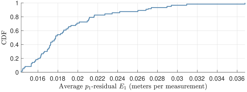
Figure 6: CDF of the average $p_{1}$ residual for the experiment with 100 nodes. The span of values has of 0.035 m per measurement, slightly better than the 0.085 m per measurement from the previous experiment in Fig. 2.

A similar observation can be drawn from Fig. 6 regarding the more challenging of the two relaxations we performed. We note that both of the residuals per measurement are smaller with larger networks.

Conclusions

We presented a non-canonical relaxation of the hybrid network localization problem, with excellent accuracy, and where optimality certificates correlate with positioning error, informing on the quality of the approximate solution.

References

- [1] L. Paull, S. Saeedi, M. Seto, and H. Li, “AUV navigation and localization: A review,” IEEE Journal of Oceanic Engineering, vol. 39, no. 1, pp. 131–149, 2014.
- [2] D. Schneider, “You are here,” IEEE Spectrum, vol. 50, no. 12, pp. 34–39, Dec. 2013.
- [3] V. Moustaka, A. Vakali, and L. G. Anthopoulos, “A systematic review for smart city data analytics,” ACM Computing Surveys (CSUR), vol. 51, no. 5, p. 103, 2019.
- [4] K. Witrisal, P. Meissner, E. Leitinger, Y. Shen, C. Gustafson, F. Tufvesson, K. Haneda, D. Dardari, A. F. Molisch, A. Conti, and M. Z. Win, “High-accuracy localization for assisted living: 5G systems will turn multipath channels from foe to friend,” IEEE Signal Process. Mag., vol. 33, no. 2, pp. 59–70, Mar. 2016.
- [5] C. E. O’Lone, H. S. Dhillon, and R. M. Buehrer, “A statistical characterization of localization performance in wireless networks,” IEEE Transactions on Wireless Communications, pp. 1–1, 2018.
- [6] F. Al-Turjman, “Positioning in the internet of things era: An overview,” in 2017 International Conference on Engineering and Technology (ICET), Aug 2017, pp. 1–5.
- [7] M. S. Hossain, “Cloud-supported cyber–physical localization framework for patients monitoring,” IEEE Systems Journal, vol. 11, no. 1, pp. 118–127, March 2017.
- [8] N. Dey, A. S. Ashour, F. Shi, and R. S. Sherratt, “Wireless capsule gastrointestinal endoscopy: Direction-of-arrival estimation based localization survey,” IEEE Reviews in Biomedical Engineering, vol. 10, pp. 2–11, 2017.
- [9] J. Aspnes, T. Eren, D. K. Goldenberg, A. S. Morse, W. Whiteley, Y. R. Yang, B. D. Anderson, and P. N. Belhumeur, “A theory of network localization,” IEEE Transactions on Mobile Computing, vol. 5, no. 12, pp. 1663–1678, 2006.
- [10] X. Ji and H. Zha, “Sensor positioning in wireless ad-hoc sensor networks using multidimensional scaling,” in IEEE INFOCOM 2004, vol. 4. IEEE, 2004, pp. 2652–2661.
- [11] W. Jiang, C. Xu, L. Pei, and W. Yu, “Multidimensional scaling-based TDOA localization scheme using an auxiliary line.” IEEE Signal Process. Lett., vol. 23, no. 4, pp. 546–550, 2016.
- [12] C. Soares, J. Xavier, and J. Gomes, “Distributed, simple and stable network localization,” in Signal and Information Processing (GlobalSIP), 2014 IEEE Global Conference on, Dec 2014, pp. 764–768.
- [13] S. Zhou, N. Xiu, and H. Qi, “A fast matrix majorization-projection method for penalized stress minimization with box constraints,” IEEE Transactions on Signal Processing, vol. 66, no. 16, pp. 4331–4346, Aug 2018.
- [14] A. Simonetto and G. Leus, “Distributed maximum likelihood sensor network localization,” Signal Processing, IEEE Transactions on, vol. 62, no. 6, pp. 1424–1437, Mar. 2014.
- [15] C. Soares, J. Xavier, and J. Gomes, “Simple and fast convex relaxation method for cooperative localization in sensor networks using range measurements,” Signal Processing, IEEE Transactions on, vol. 63, no. 17, pp. 4532–4543, Sept 2015.
- [16] N. Piovesan and T. Erseghe, “Cooperative localization in wsns: a hybrid convex/non-convex solution,” IEEE Transactions on Signal and Information Processing over Networks, vol. PP, no. 99, pp. 1–1, 2016.
- [17] Q. Shi, C. He, H. Chen, and L. Jiang, “Distributed wireless sensor network localization via sequential greedy optimization algorithm,” Signal Processing, IEEE Transactions on, vol. 58, no. 6, pp. 3328 –3340, June 2010.
- [18] K. K. Saab and S. S. Saab, “Application of an optimal stochastic Newton-Raphson technique to triangulation-based localization systems,” in 2016 IEEE/ION Position, Location and Navigation Symposium (PLANS), April 2016, pp. 981–986.
- [19] M. Agiwal, A. Roy, and N. Saxena, “Next generation 5G wireless networks: A comprehensive survey,” IEEE Communications Surveys Tutorials, vol. 18, no. 3, pp. 1617–1655, thirdquarter 2016.
- [20] Y. Shen and M. Z. Win, “Fundamental limits of wideband localization — Part I: A general framework,” IEEE Trans. Inf. Theory, vol. 56, no. 10, pp. 4956–4980, Oct. 2010.
- [21] N. Patwari, J. N. Ash, S. Kyperountas, A. O. Hero, R. L. Moses, and N. S. Correal, “Locating the nodes: cooperative localization in wireless sensor networks,” IEEE Signal processing magazine, vol. 22, no. 4, pp. 54–69, 2005.
- [22] P. Biswas, H. Aghajan, and Y. Ye, “Integration of angle of arrival information for multimodal sensor network localization using semidefinite programming,” in Proceedings of the 39th Annual Asilomar Conference on Signals, Systems, and Computers, Pacific Grove, CA, USA, 2005.
- [23] T. Eren, “Cooperative localization in wireless ad hoc and sensor networks using hybrid distance and bearing (angle of arrival) measurements,” EURASIP Journal on Wireless Communications and Networking, vol. 2011, no. 1, p. 72, 2011.
- [24] B. Q. Ferreira, J. Gomes, and J. P. Costeira, “A unified approach for hybrid source localization based on ranges and video,” in 2015 IEEE International Conference on Acoustics, Speech and Signal Processing (ICASSP), April 2015, pp. 2879–2883.
- [25] B. Ferreira, J. Gomes, C. Soares, and J. P. Costeira, “Collaborative localization of vehicle formations based on ranges and bearings,” in 2016 IEEE Third Underwater Communications and Networking Conference (UComms), Aug 2016, pp. 1–5.
- [26] H. Naseri and V. Koivunen, “Convex relaxation for maximum-likelihood network localization using distance and direction data,” in 2018 IEEE 19th International Workshop on Signal Processing Advances in Wireless Communications (SPAWC), June 2018, pp. 1–5.
- [27] B. Q. Ferreira, J. Gomes, C. Soares, and J. P. Costeira, “FLORIS and CLORIS: Hybrid source and network localization based on ranges and video,” Signal Processing, vol. 153, pp. 355–367, 2018.
- [28] Y. Wu, B. Peng, H. Wymeersch, G. Seco-Granados, A. Kakkavas, M. H. C. Garcia, and R. A. Stirling-Gallacher, “Cooperative localization with angular measurements and posterior linearization,” arXiv preprint arXiv:1907.04700, 2019.
- [29] S. M. Kay, Fundamentals of Statistical Signal Processing - Estimation Theory. Prentice Hall, 1993, vol. I.
- [30] P. Oğuz-Ekim, J. Gomes, J. Xavier, and P. Oliveira, “Robust localization of nodes and time-recursive tracking in sensor networks using noisy range measurements,” Signal Processing, IEEE Transactions on, vol. 59, no. 8, pp. 3930 –3942, Aug. 2011.
- [31] S. Tomic, M. Beko, and M. Tuba, “A linear estimator for network localization using integrated RSS and AoA measurements,” IEEE Signal Processing Letters, vol. 26, no. 3, pp. 405–409, 2019.
- [32] S. Tomic, M. Beko, R. Dinis, and J. Gomes, “Target tracking with sensor navigation using coupled RSS and AOA measurements,” Sensors, vol. 17, no. 11, p. 2690, 2017.
- [33] B. D. O. Anderson, I. Shames, G. Mao, and B. Fidan, “Formal theory of noisy sensor network localization,” SIAM Journal on Discrete Mathematics, vol. 24, no. 2, pp. 684–698, 2010.
- [34] M. Grant and S. Boyd, “CVX: Matlab software for disciplined convex programming, version 1.21,” http://cvxr.com/cvx, Apr. 2011.