Accent-Robust Automatic Speech Recognition Using Supervised and Unsupervised Wav2vec Embeddings

Abstract

Speech recognition models often obtain degraded performance when tested on speech with unseen accents. Domain-adversarial training (DAT) and multi-task learning (MTL) are two common approaches for building accent-robust ASR models. ASR models using accent embeddings is another approach for improving robustness to accents. In this study, we perform systematic comparisons of DAT and MTL approaches using a large volume of English accent corpus (4000 hours of US English speech and 1244 hours of 20 non-US-English accents speech). We explore embeddings trained under supervised and unsupervised settings: a separate embedding matrix trained using accent labels, and embeddings extracted from a fine-tuned wav2vec model. We find that our DAT model trained with supervised embeddings achieves the best performance overall and consistently provides benefits for all testing datasets, and our MTL model trained with wav2vec embeddings are helpful learning accent-invariant features and improving novel/unseen accents. We also illustrate that wav2vec embeddings have more advantages for building accent-robust ASR when no accent labels are available for training supervised embeddings.

Index Terms—  accent ASR, unsupervised embeddings, wav2vec, domain-adversarial training, multi-task learning

1 Introduction

Automatic speech recognition (ASR) models are expected to be robust to different domains, such as speaker characteristics, accents, dialects, and environmental noise. Nevertheless, ASR models often obtain inferior performance when tested on input from unseen domains. For example, ASR models pretrained on a US English accent don’t generalize well on data from other English accents [1, 2]. To tackle such problems, transfer learning has drawn a lot of attention in recent studies [3, 4]. The key insight of transfer learning is to leverage knowledge learned from a rich-resourced domain and adapt to a lower-resourced domain. Its ultimate goal is to reduce the mismatch of the data distributions between the source data (usually rich-resourced) and target data (usually lower-resourced). In our study, the rich-resourced data is US-English accented speech, and the lower-resourced data is non-US-English accented speech.

Domain-adversarial training (DAT) [5] has been demonstrated to be beneficial for transfer learning in speech processing [6, 7, 8]. DAT maps all input domains into a non-discriminative latent space, so the model is able to reuse this latent space for improving performance to unseen input domains. A similar DAT-based approach for learning an accent-invariant representation is to use generative-adversarial nets (GAN) to disentangle accent-invariant and accent-specific acoustic information [9]. In contrast to DAT, multi-task learning (MTL) with accent recognition as an auxiliary task is another common approach for building accent-robust ASR. Many studies discovered that introducing accent embeddings, such as i-vectors [10] and x-vectors [11] that are known helpful for speaker recognition, as part of input features is another major key to obtain improvements for accented speech [2, 12, 13, 14]. Recently, unsupervised accent modeling has shown to be beneficial for improving accented English speech [15, 16]. Past studies has investigated the advantages using DAT and MTL on accented speech and unseen accents. [8] found that TDNN-based model trained with DAT was consistently superior than MTL on accented Mandarin speech. [15] showed that RNN-T system, trained on multi-accent English data with DAT, achieved significant improvements on unseen English accents by relabeling one-hot accent labels with unsupervised cluster or soft labels generated from accent classifier.

Wav2vec (2.0) [17, 18] comprises a set of recently proposed models that learn hidden embeddings from massive amounts of untranscribed speech using contrastive loss in an unsupervised learning setting. Its use has resulted in improvement on acoustic modeling for ASR tasks. Several studies also discover that fine-tuned wav2vec embeddings can be beneficial for speech emotion recognition [19], speaker verification and language identification [20] and speech recognition [21].

In our experiments, we train a transformer-based CTC [22] model and demonstrate effectiveness of DAT/MTL learning accent-invariant features. We further quantify the advantages using wav2vec embeddings over labeled embeddings in our ablation study. Specifically, this paper makes the following novel contributions:

• We test our models on a large volume of real-world data containing 21 English accents. Note that previous studies usually had less than 10 accents.

• We systematically compare both supervised and unsupervised wav2vec embeddings on DAT and MTL models.

• We introduce different percentages of corrupted labels for supervised labeled embeddings to illustrate the benefit of using unsupervised wav2vec embeddings.

2 Data

Our full dataset consists of about 17k-hours of audio extracted from de-identified public English videos with no personal identifiable information. To protect users’ privacy, we cannot make this dataset public. We first augment the full dataset using speed perturbation [23] and segment it into 10s-long chunks to yield an overall dataset of size 52k hours. In this project, for training data, we selected 10% of the augmented data to match the original accent distributions of the full dataset. Table 1 shows the training and testing data distributions for each accent. en_gb has accents from England, Ireland and Scotland. All accent labels other than en_us in our dataset were manually annotated. For the testing datasets (“video-types”), en_us consists of clean (24h), noisy (23h), and extreme (46h) audio; all other accents have the noisy condition only.

[] Accent Train Test Accent Train Test en_us (US) 4000 92.5 en_gb (UK) 269.8 23.2 en_au (Australia) 249.1 23.3 en_in (India) 142.1 16.8 en_en (England) 136.7 23.2 en_ie (Ireland) 48.0 19.9 en_kr (Korea) 46.8 20.1 en_vn (Vietnam) 42.8 15.8 en_co (Colombia) 41.6 17.6 en_ph (Philippine) 40.0 16.2 en_fr (France) 34.9 25.1 en_br (Brazil) 33.6 17.7 en_mx (Mexico) 33.0 15.4 en_ca (Canada) 31.7 19.6 en_ke (Kenya) 23.5 17.7 en_za (South Africa) 16.8 19.0 en_ng (Nigerian) 16.7 16.3 en_eg (Egypt) 13.1 16.9 en_sq (Scotland) 13.1 9.5 en_pk (Pakistan) 8.4 15.7 en_ar (Argentina) 2.7 9.7

Table 1: Training and testing data distributions for accents, in hours.

For preprocessing data, we extract 80-dimensional log-mel filter energies every 10ms from each utterance. We also encode transcriptions from an inventory of 5000 word pieces, which is the output vocabulary of our ASR model. The word pieces are obtained by training a sentence piece model [24] on the US English transcripts.

3 Model

Figure 1 shows our ASR architecture, a transformer-based CTC architecture with intermediate CTC loss [25]. The encoder consists of 3 VGG [26] layers and 24 transformer layers. Three VGG layers, each of which has convolutional kernel size 3 and pooling size 2, with increasing number of channels (32, 64, and 128), are used to downsample by a factor of 8 input logmel filterbanks and extract acoustic information. The output of the VGG layers is fed into a linear layer with output dimension 512. Auxiliary embeddings, if used, are either concatenated or weighted summed to the output of linear layer. The combined output is fed into 24 transformer layers to predict word pieces using a CTC loss. Each transformer layer has 8 multi-attention heads with hidden dimension 2048. To enhance ASR performance, we use 3 intermediate CTC losses at the 6${}^{\text{th}}$, 12${}^{\text{th}}$, and 18${}^{\text{th}}$ transformer layers. We place an accent classifier at the 7${}^{\text{th}}$ transformer layer, as we empirically observe it performs better than in other positions (layer 13, 19 and 24). Each CTC loss and accent classifier is composed of two layers: one linear layer with output dimension of 256 followed by ReLU activation + one softmax layer.

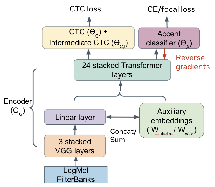
Fig. 1: Overall model architecture.

We denote $\mathbf{x}$ as the input logmel filterbanks, $\mathbf{y}$ as the word pieces encoded by transcriptions, $\mathbf{y_{a}}$ as the corresponding accent labels, and $N$ as the number of accents. The training objective can be written as Equation (1), where $\mathcal{L}_{CTC}(\mathbf{x,y})$ is the CTC loss, $\mathcal{L}_{CTC,l}(\mathbf{x,y})$ is the CTC intermediate loss, and $\mathcal{L}_{acc}(\mathbf{x,y_{a}})$ is the cross-entropy (CE)/focal loss of accent classifier. We denote $\theta_{E}$, $\theta_{C}$, $\theta_{C,l}$ and $\theta_{A}$ as the parameters of encoder, CTC loss, CTC intermediate loss, and accent classifier respectively. Let $\lambda$ and $\beta$ be weights of intermediate CTC loss and gradient reversal respectively. Equations (2)-(5) show the updated rules used in our experiments, and only the gradients of the accent classifier loss are reversed. Equation (6) specifies the computation for cross-entropy(CE)/focal loss.

$$\mathcal{L} =\mathcal{L}_{CTC}(\mathbf{x,y})+\lambda\sum_{l}\mathcal{L}_{CTC,l}(\mathbf{x,y})+\beta\mathcal{L}_{acc}(\mathbf{x,y_{a}})$$ (1)

$$\theta_{E} \xleftarrow[]{}\theta_{E}-(\frac{\partial\mathcal{L}_{CTC}}{\partial\theta_{E}}+\lambda\frac{\partial\mathcal{L}_{CTC,l}}{\partial\theta_{E}}-\beta\frac{\partial\mathcal{L}_{acc}}{\partial\theta_{E}})$$ (2)

$$\theta_{C} \xleftarrow[]{}\theta_{C}-\frac{\partial\mathcal{L}_{CTC}}{\partial\theta_{C}}$$ (3)

$$\theta_{C,l} \xleftarrow[]{}\theta_{C,l}-\lambda\frac{\partial\mathcal{L}_{CTC,l}}{\partial\theta_{C,l}}$$ (4)

$$\theta_{A} \xleftarrow[]{}\theta_{A}-\beta\frac{\partial\mathcal{L}_{acc}}{\partial\theta_{A}}$$ (5)

$$\mathcal{L}_{acc} =\begin{cases}-\sum_{i=1}^{N}y_{i}\log(P(y_{i}|x_{i}))&\text{CE loss}\\ -\sum_{i=1}^{N}-(1-P(y_{i}|x_{i}))^{\gamma}\log(P(y_{i}|x_{i}))&\text{Focal loss}\\ \end{cases}$$ (6)

In our experiments, we test our data on three models, including a baseline system, DAT and MTL, and we test each model with and without auxiliary embeddings. Our baseline model consists of an encoder, a CTC loss and three CTC intermediate losses without auxiliary embeddings. DAT/MTL has all components of baseline + accent classifier with/without gradient reversal layer respectively.

4 Experimental Settings

We perform two sets of experiments: 1) “all”: this setting trains the model with all 21 accents data and evaluates using 20 non en_us testing data and all en_us testing video types; 2) “s18”: this setting trains the model with data from 18 accents, excluding en_ar (very low-resource), en_eg (low-resource), and en_ph (middle-resource), and evaluates using 17 non en_us accents, 3 novel accents, and all en_us testing video types. By partitioning our dataset into seen/unseen accents for training and testing, we are able to verify the effectiveness of DAT to learn accent-invariant features and of MTL to learn latent accent representation. For novel accents, we didn’t choose all of them to be among the lowest-resourced range to reduce the chance of insufficient test data for learning accent-invariant features. For all the experiments, we run 100 epochs with 16 GPUs in parallel. We use Adam as our optimizer with an initial learning rate of 0.0012 and forced annealing after epoch 50 by a factor of 0.95. For training the DAT model, we find that setting $\beta>0$ for all training epochs over-trains the accent classifier and fails to learn accent-invariant features. Thus, we set $\beta=0$ for the first 50 epochs to first train the accent classifier until convergence, and then we set $\beta>0$ for the last 50 epochs to back-prop reversed gradients to the encoder. In this way, we observe our accent classifier effectively bring down accent recognition accuracy to around 10% for the last 50 epochs. For CE loss, we set $\beta=0.03$ and $\lambda=0.3$. For focal loss, we set $\beta=1,\gamma=0.5$, and $\lambda=0.3$. For inference, we use a FST-based decoder with the HLG graph built following the approach in [27]. We use a 5-gram language model trained on 14k hours of en_us transcripts.

4.1 Supervised labeled embeddings

We use a separate trainable matrix, $\mathbf{W}_{labeled}\in R^{N\times D}$, as side input, where $N$ is the number of accents in training data and $D$ is the dimension of the hidden embedding. Each row of $\mathbf{W}_{labeled}$ corresponds to an accent, and corresponding rows are either concatenated or weighted and summed to the output of the linear layer. Define $M$ as the hidden dimension of the output of linear layer in the ASR model. We set $D=64$ and $M=448$ for concatenation layer so that the labeled embeddings take a relatively smaller part of the combined features, $D=512$ and $M=512$ for weighted sum layer so that dimensions of the input features and auxiliary embeddings are summable. Similarly, for the wav2vec embeddings (see section 4.2), $D=64$ and $M=448$ for the concatenation layer, and $D=768$ and $M=768$ for the weighted sum layer as $D=768$ is the original setting of the wav2vec model. For both types of embeddings, we set the weight as 0.2 for the weighted sum layer.

4.2 Unsupervised wav2vec embeddings

We use the pretrained wav2vec model from [20] that consists of 24 transformer layers and learns hidden embeddings from 25 languages of untranscribed speech. We fine-tune the wav2vec model using our training data by adding an average time pooling layer for producing utterance-level embeddings and a softmax layer for classifying accents. We then extract hidden embeddings from the average time pooling layer as our auxiliary embeddings, $\mathbf{W}_{w2v}$. To achieve the best accent classification accuracy on the validation set, we fine-tune with weighted data samplers by assigning more weight on en_us accent data and equal weights across non en_us accents. For example, we balance our training set with 20% for en_us, and 80% for 20 other non en_us accents (4% each). We achieve the best accent recognition accuracy (for all: 74.41% when D=768 and 75.17% when D=64; for s18: 70.71% when D=768 and 70.75% when D=64) when en_us is assigned 10% weight and 20 other accents are assigned 90% (4.5% each). We confirm that our wav2vec embeddings contain useful accent information based on the visualizations shown in Figure 2. We z-normalize wav2vec embeddings before concatenating or weighted summing it to the output of the linear layer.

4.3 Visualizations of wav2vec embeddings and accent remap

To visualize wav2vec embeddings, we randomly select 300 en_us embeddings and 100 examples from each of the non en_us embeddings. We first apply Linear Discriminant Analysis to the wav2vec embeddings and reduce the embedding dimension from 768 to 5, and then we apply T-SNE [28] with default settings in the sklearn package [29] to those reduced-dimension embeddings. Figure 2 shows T-SNE plot of embeddings extracted from a wav2vec model pretrained with 8 transformer layers and fine-tuned with all accent labels using CE loss. Based on Figure 2, accents can be grouped by their regions, such as Europe (en_au, en_en, en_ie, en_gb, and en_sq), North America (en_us and en_ca), Africa (en_za, en_ke, and en_ng), South America (en_ar, en_br, en_mx, and en_co), Southeast Asia (en_ph), South Asia (en_in and en_pk), East Asia (en_kr), Northeast Africa (en_eg), and Europe/South Asia (en_fr and en_vn). Although en_fr and en_vn are not geographically close, 80 years of French colonial rule lead to various loanwords of Vietnamese from French [30]. We thus assign them to one group. To utilize accent regional information, we remap each accent into larger groups to obtain another set of labels. We observe that en_co is closer to the European group rather than the South America group, so we assign en_co into the European group. For s18 setting, three novel accents are remapped to the closest group (South America) based on Figure 2.

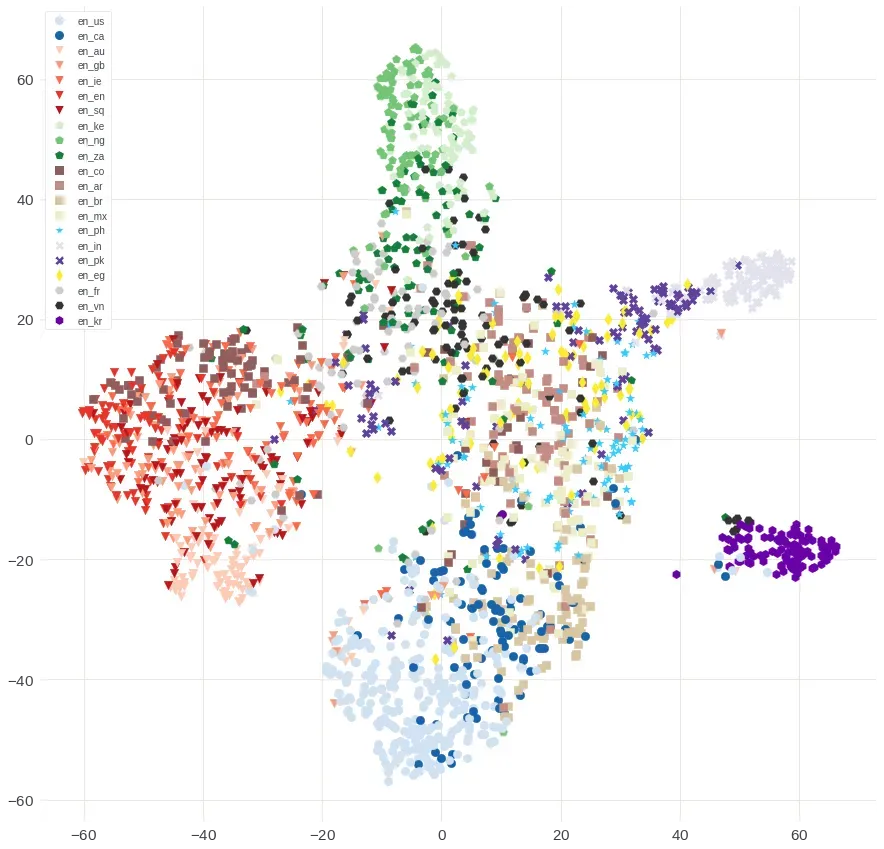
Fig. 2: T-SNE plot of wav2vec embeddings. Accents from different regions are labeled with different shapes; accents within the same region are labeled with different ranges of the same color.

5 Results

5.1 Baseline results

Table 2 shows performance on the baseline model trained with en_us data alone versus en_us + 20 non en_us accent data. Training including accented data significantly improves non en_us word error rates (WER) and slightly benefits en_us WER. We had observed that previous work (e.g., [2]) typically showed much larger degradation on accented speech when trained only on US-accented speech. We suspected that our en_us data contained some amount of accented speech. To check this, we ran a wav2vec accent classifier (section 4.2), and did find small amounts (2%) of accented data. This may partially contribute to the smaller than expected performance gap.

[] model training data non en_us en_us baseline en_us only 21.7 17.7 baseline en_us + non en_us 17.0 17.3

Table 2: Average WER, in percent (%), for baseline model without auxiliary embedding trained on en_us only and en_us + non en_us dataset.

5.2 Embeddings effects on baseline, DAT and MTL models

Table 3 summarizes important results for experiments without auxiliary embeddings. Models trained with focal loss (DAT1-F and MTL1-F) achieve the best results on en_us testing data and comparable results on non en_us data in both all and s18 settings, compared with CE loss (DAT1-CE and MTL1-CE). MTL1-CE shows worse results than the baseline (B1). Thus, we train the rest of the experiments using focal loss.

[] model accent non en_us novel en_us loss all s18 s18 all s18 B1: baseline - 17.0 16.5 21.2 17.3 17.1 DAT1-CE CE 16.9 16.3 21.1 17.2 17.1 MTL1-CE 17.1 17.0 21.1 17.3 17.2 DAT1-F focal 17.0 16.4 21.3 17.0 17.0 MTL1-F 16.9 16.4 21.2 17.1 17.0

Table 3: Average WER for baseline, DAT and MTL without embeddings. Models are named with initials+numbers+accent classifier loss settings, e.g, DAT1-CE means DAT trained with CE loss. The best result for each setting is bolded across Table 3 and 4.

Table 4 presents results of baseline, DAT and MTL models using embeddings. We observe that B2-labeled(C) is generally better than B2-labeled(S), while B2-w2v(S) is generally better than B2-w2v(C), which can be due to the mismatch distributions between the input features and wav2vec embeddings. Thus, we keep this setting for the rest of the experiments. DAT2-labeled(C), our overall best model, shows equal or superior performances than MTL2-labeled(C) and B2-labeled(C) for all testing datasets, which demonstrates the effectiveness of DAT learning accent-invariant information. We find that MTL2-labeled(C) is not better than B2-labeled(C), which suggests that the accent classifier is not essential when we feed ground-truth labeled embeddings as part of the input. However, accent classifier is helpful when we feed wav2vec embeddings, as MTL2-w2v(S) benefits novel accents the most than other models using wav2vec embeddings. For experiments using the accent remap technique, regional information is mainly beneficial for DAT3-w2v(S) and MTL3-w2v(S) trained on non en_us and en_us datasets, compared to corresponding settings without accent remap (DAT2-w2v(S) and MTL2-w2v(S)). A typical trend of our results in Table 4 is that we have slightly worse performances on en_us and relatively small improvements on non en_us and novel accents compared to our baseline. This may be explained by 1) our en_us training data is contaminated by a small amount of other accents (see section 5.1), and 2) comparing against a baseline model trained on multi-accent data yields smaller improvements as opposed to comparing against a single yet mismatched accent model. Similar trends can be found in [15]: DAT yields smaller improvements on unseen en-AU accent data over the “data pooling” baseline compared to accent-specific models with individual accent embeddings.

[] model non en_us novel en_us all s18 s18 all s18 B1: baseline 17.0 16.5 21.2 17.3 17.1 B2-labeled(C) 16.4 15.9 20.9 17.3 17.3 B2-labeled(S) 16.5 16.1 21.4 17.0 17.3 B2-w2v(C) 17.0 16.4 21.2 17.1 17.4 B2-w2v(S) 16.7 16.4 21.1 17.3 17.3 DAT2-labeled(C) 16.4 15.9 20.9 17.1 17.2 MTL2-labeled(C) 16.5 16.7 21.0 17.2 17.4 DAT2-w2v(S) 16.9 16.4 21.1 17.3 17.6 MTL2-w2v(S) 16.9 16.3 21.0 17.1 17.5 DAT3-labeled(C) 16.8 16.4 21.1 17.4 17.5 MTL3-labeled(C) 16.7 16.3 21.0 17.0 17.1 DAT3-w2v(S) 16.8 16.4 21.1 17.1 17.2 MTL3-w2v(S) 16.8 16.4 21.3 17.1 17.1

Table 4: Average WER for baseline, DAT and MTL with labeled/wav2vec embeddings using focal loss. C means concatenation layer; S means weighted sum layer, as described in Section 3. Models are named with initials+numbers+embedding, e.g, DAT2-labeled(C) means DAT trained with labeled embeddings in concatenation layer (C). Groups of DAT3 and MTL3 are experiments using accent remap technique. The best result for each setting is bolded across Table 3 and 4.

5.3 Ablation study of corrupted labels on labeled embeddings

Although we achieve the best performance with supervised labeled embeddings, we may not always have accurate accent labels available. To understand the effects of accurate labels, we perform an ablation study by introducing different amounts of corrupted labels for labeled embeddings during inference. For generating corrupted labels, we use random and incorrect labels replacing part of the ground-truth labels for non en_us and en_us datasets in both all and s18 settings. Because ground-truth labels are not defined for novel accents in s18, we test two types of embeddings for its ground-truth: 1) untrained embeddings that are randomly initialized and 2) en_us embeddings. Table 5 shows relevant results. With more corrupted labels, WER increases across three testing datasets as expected. We can estimate that if 10-25% of the labels are corrupted, wav2vec embeddings will have superior performances than labeled embeddings. For novel accents, untrained embeddings are more helpful than en_us embeddings even though en_us embeddings are better trained.

[] non en_us novel en_us all s18 s18* $\textit{s18}^{\dagger}$ all s18 0% 16.4 15.9 20.9 21.6 17.3 17.3 10% 16.6 16.2 20.9 21.6 17.3 17.2 25% 16.9 16.5 21.1 21.6 17.4 17.3 50% 17.4 16.9 21.3 21.6 17.4 17.3 B2-w2v(S) 16.7 16.4 21.1 - 17.3 17.3

Table 5: Average WER for B2-labeled(C) trained with different percentage of corrupted labels. Novel accents labels were tested for both untrained(*) and en_us($\dagger$) embeddings. Results for B2-w2v(S) are copied to the last row for easy comparisons.

6 Conclusion

We investigate three transformer-based CTC models: baseline, DAT and MTL, and we test each model with two types of embeddings, supervised and unsupervised wav2vec embeddings, on a dataset consisting of en_us accent and 20 non en_us accents. We find that DAT trained with labeled embeddings encourages the model to learn accent-invariant features and provides benefits across all testing datasets. MTL trained with wav2vec embeddings performs the best for novel accents among all other corresponding models. We show that using wav2vec embeddings is beneficial when no accent labels are available for training labeled embeddings, and results from our ablation study illustrate that wav2vec embeddings are better than labeled embeddings when 10-25% accent training labels are corrupted.

References

- [1] Abhinav Jain, Minali Upreti, and Preethi Jyothi, “Improved accented speech recognition using accent embeddings and multi-task learning.,” in Interspeech, 2018, pp. 2454–2458.
- [2] Mehmet Ali Tuğtekin Turan, Emmanuel Vincent, and Denis Jouvet, “Achieving multi-accent asr via unsupervised acoustic model adaptation,” in Interspeech, 2020.
- [3] Jaejin Cho, Murali Karthick Baskar, et al., “Multilingual sequence-to-sequence speech recognition: architecture, transfer learning, and language modeling,” in IEEE Spoken Language Technology Workshop (SLT). IEEE, 2018, pp. 521–527.
- [4] Julius Kunze, Louis Kirsch, Ilia Kurenkov, Andreas Krug, Jens Johannsmeier, and Sebastian Stober, “Transfer learning for speech recognition on a budget,” arXiv preprint arXiv:1706.00290, 2017.
- [5] Yaroslav Ganin, Evgeniya Ustinova, Hana Ajakan, Pascal Germain, Hugo Larochelle, François Laviolette, Mario Marchand, and Victor Lempitsky, “Domain-adversarial training of neural networks,” The journal of machine learning research, vol. 17, no. 1, pp. 2096–2030, 2016.
- [6] Chien-Feng Liao, Yu Tsao, Hung-Yi Lee, and Hsin-Min Wang, “Noise adaptive speech enhancement using domain adversarial training,” arXiv preprint arXiv:1807.07501, 2018.
- [7] Qing Wang, Wei Rao, Sining Sun, Leib Xie, Eng Siong Chng, and Haizhou Li, “Unsupervised domain adaptation via domain adversarial training for speaker recognition,” in Proc. ICASSP. IEEE, 2018, pp. 4889–4893.
- [8] Sining Sun, Ching-Feng Yeh, Mei-Yuh Hwang, Mari Ostendorf, and Lei Xie, “Domain adversarial training for accented speech recognition,” in Proc. ICASSP. IEEE, 2018, pp. 4854–4858.
- [9] Yi-Chen Chen, Zhaojun Yang, Ching-Feng Yeh, Mahaveer Jain, and Michael L Seltzer, “Aipnet: Generative adversarial pre-training of accent-invariant networks for end-to-end speech recognition,” in Proc. ICASSP. IEEE, 2020, pp. 6979–6983.
- [10] Najim Dehak, Patrick J Kenny, Réda Dehak, Pierre Dumouchel, and Pierre Ouellet, “Front-end factor analysis for speaker verification,” IEEE Transactions on Audio, Speech, and Language Processing, vol. 19, no. 4, pp. 788–798, 2010.
- [11] David Snyder, Daniel Garcia-Romero, et al., “X-vectors: Robust dnn embeddings for speaker recognition,” in Proc. ICASSP. IEEE, 2018, pp. 5329–5333.
- [12] Thibault Viglino, Petr Motlicek, and Milos Cernak, “End-to-end accented speech recognition.,” in Interspeech, 2019, pp. 2140–2144.
- [13] Wenbi Rao, Ji Zhang, and Jianwei Wu, “Improved blstm rnn based accent speech recognition using multi-task learning and accent embeddings,” in Proceedings of the 2020 2nd International Conference on Image, Video and Signal Processing, 2020, pp. 1–6.
- [14] Mingming Chen, Zhanlei Yang, Jizhong Liang, Yanpeng Li, and Wenju Liu, “Improving deep neural networks based multi-accent mandarin speech recognition using i-vectors and accent-specific top layer,” in Interspeech, 2015.
- [15] Hu Hu, Xuesong Yang, Zeynab Raeesy, Jinxi Guo, Gokce Keskin, Harish Arsikere, Ariya Rastrow, Andreas Stolcke, and Roland Maas, “Redat: Accent-invariant representation for end-to-end ASR by domain adversarial training with relabeling,” in Proc. ICASSP, 2021.
- [16] Song Li, Beibei Ouyang, Dexin Liao, Shipeng Xia, Lin Li, and Qingyang Hong, “End-to-end multi-accent speech recognition with unsupervised accent modelling,” in Proc. ICASSP, 2021, pp. 6418–6422.
- [17] Steffen Schneider, Alexei Baevski, Ronan Collobert, and Michael Auli, “wav2vec: Unsupervised pre-training for speech recognition,” arXiv preprint arXiv:1904.05862, 2019.
- [18] Alexei Baevski, Henry Zhou, Abdelrahman Mohamed, and Michael Auli, “wav2vec 2.0: A framework for self-supervised learning of speech representations,” arXiv preprint arXiv:2006.11477, 2020.
- [19] Leonardo Pepino, Pablo Riera, and Luciana Ferrer, “Emotion recognition from speech using wav2vec 2.0 embeddings,” arXiv preprint arXiv:2104.03502, 2021.
- [20] Andros Tjandra, Diptanu Gon Choudhury, Frank Zhang, Kritika Singh, Alexei Baevski, Assaf Sela, Yatharth Saraf, and Michael Auli, “Improved language identification through cross-lingual self-supervised learning,” arXiv preprint arXiv:2107.04082, 2021.
- [21] Alexei Baevski, Wei-Ning Hsu, Alexis Conneau, and Michael Auli, “Unsupervised speech recognition,” arXiv preprint arXiv:2105.11084, 2021.
- [22] Alex Graves, Santiago Fernández, Faustino Gomez, and Jürgen Schmidhuber, “Connectionist temporal classification: labelling unsegmented sequence data with recurrent neural networks,” in Proc. ICML, 2006, pp. 369–376.
- [23] Tom Ko, Vijayaditya Peddinti, Daniel Povey, and Sanjeev Khudanpur, “Audio augmentation for speech recognition,” in Interspeech, 2015.
- [24] Taku Kudo and John Richardson, “Sentencepiece: A simple and language independent subword tokenizer and detokenizer for neural text processing,” arXiv preprint arXiv:1808.06226, 2018.
- [25] Andros Tjandra, Chunxi Liu, et al., “Deja-vu: Double feature presentation and iterated loss in deep transformer networks,” in Proc. ICASSP. IEEE, 2020, pp. 6899–6903.
- [26] Karen Simonyan and Andrew Zisserman, “Very deep convolutional networks for large-scale image recognition,” arXiv preprint arXiv:1409.1556, 2014.
- [27] Frank Zhang, Yongqiang Wang, Xiaohui Zhang, Chunxi Liu, Yatharth Saraf, and Geoffrey Zweig, “Faster, Simpler and More Accurate Hybrid ASR Systems Using Wordpieces,” in Proc. Interspeech 2020, 2020, pp. 976–980.
- [28] Laurens Van der Maaten and Geoffrey Hinton, “Visualizing data using t-sne.,” Journal of machine learning research, vol. 9, no. 11, 2008.
- [29] Fabian Pedregosa, Gaël Varoquaux, Alexandre Gramfort, Vincent Michel, Bertrand Thirion, Olivier Grisel, Mathieu Blondel, Peter Prettenhofer, Ron Weiss, Vincent Dubourg, et al., “Scikit-learn: Machine learning in python,” the Journal of machine Learning research, vol. 12, pp. 2825–2830, 2011.
- [30] Huynh Trang Nguyen, Hemanga Dutta, et al., “The adaptation of french consonant clusters in vietnamese phonology: An ot account,” Journal of Universal Language, vol. 18, no. 1, pp. 69–103, 2017.