Accelerated Componentwise Gradient Boosting using Efficient Data Representation and Momentum-based Optimization

Abstract

Componentwise boosting (CWB), also known as model-based boosting, is a variant of gradient boosting that builds on additive models as base learners to ensure interpretability. CWB is thus often used in research areas where models are employed as tools to explain relationships in data. One downside of CWB is its computational complexity in terms of memory and runtime. In this paper, we propose two techniques to overcome these issues without losing the properties of CWB: feature discretization of numerical features and incorporating Nesterov momentum into functional gradient descent. As the latter can be prone to early overfitting, we also propose a hybrid approach that prevents a possibly diverging gradient descent routine while ensuring faster convergence. We perform extensive benchmarks on multiple simulated and real-world data sets to demonstrate the improvements in runtime and memory consumption while maintaining state-of-the-art estimation and prediction performance.

Keywords: Binning, Data Structures, Functional Gradient Descent, Machine Learning, Nesterov Momentum

1 Introduction

Model-based or componentwise boosting (CWB; Bühlmann and Yu, 2003) applies gradient boosting (Freund et al., 1996) to statistical models by sequentially adding pre-defined components to the model. These components are so-called base learners of one or multiple features. If interpretable base learners are used (e.g., univariate splines), the full CWB model remains interpretable and allows for the direct assessment of estimated partial feature effects. Further advantages of CWB are its applicability in high-dimensional feature spaces (“$p\gg n$ situations”), its inherent variable selection, and unbiased feature selection (Bühlmann and Yu, 2003; Hofner et al., 2011). It is also possible to derive inference properties of boosted estimators to quantify uncertainty using post-selection inference procedures (Rügamer and Greven, 2020). These properties make CWB a powerful method at the intersection of (explainable) statistical modelling and (black-box prediction) machine learning. For this reason, CWB is frequently used in medical research, e.g., for oral cancer prediction (Saintigny et al., 2011), detection of synchronization in bioelectrical signals (Rügamer et al., 2018), or classifying pain syndromes (Liew et al., 2020). In contrast, many other gradient boosting methods such as XGBoost (Chen and Guestrin, 2016) solely focus on predictive performance and (mainly) use tree-based base learners with higher-order interactions. As a consequence, these procedures require techniques from interpretable machine learning (see, e.g., Molnar, 2020) to explain their resulting predictions.

Various versions of the original CWB algorithm have been developed, e.g., CWB for functional data (Brockhaus et al., 2020), boosting location, scale and shape models (Hofner et al., 2016), or probing for sparse and fast variable selection (Thomas et al., 2017). CWB’s computational complexity in terms of memory and runtime is, however, a downside often encountered in practice. The high consumption of RAM of the current state-of-the-art implementation mboost (Hothorn et al., 2020) can considerably exceed the capacity of modern workstations. This makes CWB less attractive or even infeasible for medium- to large-scale applications. In this paper, we focus on two internal structures of CWB and propose improvements to mitigate these problems.

Our contributions and related literature. Our first contribution (Section 3.1) is a novel CWB modification to reduce memory consumption in large data situations. To the best of our knowledge, we are the first to derive the complexity of CWB and also the first to suggest improvements to reduce computational costs. Based on a recently proposed idea to fit generalized additive models (GAMs) on large data sets (Li and Wood, 2020), we describe adaptions of matrix operations for CWB to operate on discretized features. We refer to this approach as binning. Binning is a discretization technique for numerical features and can drastically reduce runtime and memory consumption when fitting GAMs, especially when coupled with specialized matrix operations. In contrast to Li and Wood (2020), we use binning within each base learner rather than processing the model matrix of all features. This makes the use of binning particularly beneficial for CWB.

In Section 3.2, we also adapt a novel optimization technique called Accelerated Gradient Boosting Machine (AGBM; Lu et al., 2020). AGBM allows incorporation of Nesterov momentum for gradient boosting in the function space. Based on AGBM, we propose a new variant of CWB for faster convergence while still preserving CWB’s interpretability. The adaption perfectly fits to the general optimization scheme of CWB, which is also based on functional gradient descent. However, the acceleration based on Nesterov momentum is known to diverge in certain cases (Wang et al., 2020). We thus also propose a refinement of AGBM in our algorithm Hybrid CWB (HCWB) to overcome premature divergence of the gradient descent routine.

These proposed adaptions can be applied to CWB independently of each other and are both implemented in the software package compboost (Schalk et al., 2018). In a simulation study in Section 4, we study their effect both separately and when combined. Finally, we conduct real-world benchmark experiments in Section 4 to compare our proposed CWB variants with vanilla CWB, the CWB implementation in mboost, XGBoost, and a recently published method called Explainable Boosting Machine (EBM) within the interpretML framework (Nori et al., 2019).

2 Componentwise Gradient Boosting

This section introduces the main concepts and properties of CWB as well as the notation used throughout this article.

2.1 Terminology

Consider a $p$-dimensional feature space $\mathcal{X}=(\mathcal{X}_{1}\times\ldots\times\mathcal{X}_{p})$ and a target space $\mathcal{Y}$. We assume an unknown functional relationship $f$ between $\mathcal{X}$ and $\mathcal{Y}$. ML algorithms try to learn this relationship using a training data set $\mathcal{D}=\left(\left(\mathbf{x}^{(1)},y^{(1)}\right),\ldots,\left(\mathbf{x}^{(n)},y^{(n)}\right)\right)$ with $n$ observations drawn independently from an unknown probability distribution $\mathds{P}_{xy}$ on the joint space $\mathcal{X}\times\mathcal{Y}$. Let $\hat{f}$ be the estimated model fitted on the training data to approximate $f$ and $P=\{1,\ldots,p\}$ an index set for all $p$ features. The vector $\mathbf{x}_{j}=(x_{j}^{(1)},\ldots,x_{j}^{(n)})^{\mkern-1.5mu\mathsf{T}}\in\mathcal{X}$ refers to the $j$th feature. $\mathbf{x}$ and $y$ are arbitrary members of $\mathcal{X}$ and $\mathcal{Y}$, respectively. Given $f$ and a loss function $L:\mathcal{Y}\times\mathds{R}\to\mathds{R}^{+}_{0}$, we assess the prediction quality of the model fit on the data set $\mathcal{D}$ using the empirical risk $\mathcal{R}_{\text{emp}}(f)=|\mathcal{D}|^{-1}\sum_{(\mathbf{x},y)\in\mathcal{D}}L(y,f(\mathbf{x}))$.

2.2 Base Learner

A base learner $b_{k}:\mathcal{X}\to\mathds{R}$ is used to model the contribution of one or multiple features to the estimated model $\hat{f}$. Possible base learners range from simple models like a linear model on one feature to complex models such as deep decision trees including many features. While the presented adaptions for CWB work also for multivariate base learners such as tensor product splines, we restrict ourselves to univariate functions $b_{k}(\mathbf{x},\bm{\theta})=g_{k}(x)^{\mkern-1.5mu\mathsf{T}}\bm{\theta},\bm{\theta}\in\mathds{R}^{{d_{k}}}$, for demonstration purposes. The function $g_{k}:\mathds{R}\to\mathds{R}^{d_{k}}$ is a generic representation for modeling alternatives such as linear effects, categorical effects or smooth effects. For smooth effects, numerical features are transformed using a basis representation $g_{k}(x)=(B_{k,1}(x),\dots,B_{k,{d_{k}}}(x))^{\mkern-1.5mu\mathsf{T}}$ with ${d_{k}}$ basis functions, e.g., via univariate penalized B-splines (P-Splines; Eilers and Marx, 1996). This generic representation defines a design matrix $\bm{Z}_{k}=(g_{k}(x_{j}^{(1)}),\ldots,g_{k}(x_{j}^{(n)}))^{\mkern-1.5mu\mathsf{T}}\in\mathds{R}^{n\times{d_{k}}}$ given by a feature vector $\mathbf{x}_{j}\in\mathds{R}^{n}$. Note that the base learner $b_{k}$ implicitly selects the feature(s) on which it operates without explicitly denoting the feature(s). In this paper with univariate base learners, exactly one feature is passed to the generic representation $g_{k}$. An important property induced by the choice of a linear base learner is that two base learners of the same type $b_{k}(\mathbf{x},\bm{\theta})$ and $b_{k}(\mathbf{x},\bm{\theta}^{\ast})$ sum up to one base learner of the same type:

$$b_{k}(\mathbf{x},\bm{\theta})+b_{k}(\mathbf{x},\bm{\theta}^{\ast})=b_{k}(\mathbf{x},\bm{\theta}+\bm{\theta}^{\ast}).$$ (1)

During boosting, CWB selects its next component from a pre-defined pool of base-learners $\mathcal{B}=\{b_{k}\}_{k\in\{1,\ldots,K\}}$, where in our case of univariate $b_{k}$, $K$ often equals the number of features $p$.

2.3 Componentwise Boosting

CWB estimates $\hat{f}$ using an iterative steepest descent minimization in function space. $\hat{f}^{[m]}$ denotes the prediction model after $m$ iterations. In each step, the pseudo residuals $r^{[m](i)}=-\frac{\partial L\left(y^{(i)},f\left(\mathbf{x}^{(i)}\right)\right)}{\partial f(\mathbf{x}^{(i)})}\left.\vphantom{f_{(i}^{(i}}\right|_{f=\hat{f}^{[m-1]}},\ i\in\{1,\dots,n\}$ indicate a functional gradient, evaluated at training data points, where changing the outputs of $\hat{f}^{[m]}$ reduces the overall loss of our current model, w.r.t. to the given loss $L$ the most. CWB initializes $\hat{f}^{[m]}$ with a loss-optimal constant model – also called an offset or intercept. In the $m$th iteration, all base learners in $\mathcal{B}$ are fitted against $\bm{r}^{[m]}$ via L2-loss, and the best candidate is selected to additively update $f^{[m]}$, controlled by a learning rate $\nu$. This procedure is repeated $M$ times or until a convergence criterion is met (e.g., using early stopping as described in Section 3.2.3). The details of CWB are given in Algorithm 1 in Appendix A.1.

Due to property (1) of linear base learners and the additive model update of CWB, the estimated parameter of each base learner can be summed up after $M$ iterations, and each aggregated parameter $\hat{\bm{\theta}}_{k}=\sum_{m=1}^{M}\sum_{k=1}^{K}\mathds{1}_{\{k=k^{[m]}\}}\hat{\bm{\theta}}^{[m]}$ with its base representation $g_{k}$ can be interpreted as a partial effect of the feature modeled by base learner $b_{k}$.

2.4 Computational Complexity of CWB

The computational complexity of CWB is directly related to the computational complexity of fitting each base learner. All linear base learners $b_{1},\ldots,b_{K}$ must solve a system of linear equations $\bm{Z}_{k}^{\mkern-1.5mu\mathsf{T}}\bm{Z}_{k}\bm{\theta}_{k}=\bm{Z}_{k}^{\mkern-1.5mu\mathsf{T}}\bm{r}^{[m]}$. For simplicity, assume that all base learners have the same number of parameters, i.e., ${d_{k}}=d$. Such systems are usually Cholesky decomposed with $\bm{Z}_{k}^{\mkern-1.5mu\mathsf{T}}\bm{Z}_{k}=\bm{L}_{k}\bm{L}_{k}^{\mkern-1.5mu\mathsf{T}}$, and complexity $\mathcal{O}(d^{3})$. Taking into account additional matrix operations $\bm{Z}_{k}^{\mkern-1.5mu\mathsf{T}}\bm{Z}_{k}$ with $d^{2}n$, $\bm{Z}_{k}^{\mkern-1.5mu\mathsf{T}}\bm{r}^{[m]}$ with $dn$, and forward/backward solving with $(d^{2}-d)/2$ operations, this yields a complexity of $\mathcal{O}(d^{2}n+d^{3})$. When applied to all $K$ base learners in $M$ iterations, this yields $\mathcal{O}(MK(d^{2}n+d^{3}))$ (neglecting operations such as the calculations of pseudo residuals $\bm{r}^{[m]}$ and sum of squared errors $\text{SSE}_{k}$, or finding the best base learner $k^{[m]}$).

The above can be accelerated considerably by pre-calculating the (expensive) Cholesky decomposition once for every base learner before boosting. This reduces the computational complexity of CWB to $\mathcal{O}(K(d^{2}n+d^{3}))$. When taking also the forward/backward solving and calculation of $\bm{Z}_{k}^{\mkern-1.5mu\mathsf{T}}\bm{r}^{[m]}$ as operations per iteration into account, the complexity when caching heavy operations reduces to $\mathcal{O}(K(d^{2}n+d^{3})+MK(d^{2}+dn))$.

3 A more Efficient Componentwise Boosting

3.1 Binning

In order to make CWB feasible for large data sets and reduce computational resources in general, we propose to combine CWB with binning. While the primary goal of binning is to reduce the memory consumption by representing numerical feature via discretization, this method can also accelerate the model fit.

3.1.1 Discretizing numerical Features

Binning discretizes a numerical feature into a smaller number of design point values. Usually, binned values are constructed as an equally spaced grid Lang et al. (2014) $z_{j}^{(i)}=\mathop{\sf min}(\mathbf{x}_{j})+(i-1)/(n^{\ast}-1)(\mathop{\sf max}(\mathbf{x}_{j})-\mathop{\sf min}(\mathbf{x}_{j}))$, $i=1,\dots,n^{\ast}$ and then replace each value $x_{j}^{(i)}$ with its closest design point $z_{j}^{(i)}$. The number of design points $n^{\ast}$ can be chosen arbitrarily. Wood et al. (2017) argue that the trade-off between data size and statistical error due to imprecise feature values is most adequate for $n^{\ast}=\sqrt{n}$.

Design points and index vector. Instead of storing the discretized feature vector $\tilde{\mathbf{x}}_{j}=(\tilde{x}^{(1)}_{j},\ldots,\tilde{x}^{(n)}_{j})^{\mkern-1.5mu\mathsf{T}}\in\mathds{R}^{n}$, it is sufficient to store the $n^{\ast}$ values of $\bm{z}_{j}$ as well as an additional index vector $\mathbf{ind}_{k}=(ind_{k}^{(1)},\ldots,ind_{k}^{(n)})^{\mkern-1.5mu\mathsf{T}}$ (i.e., the assignment of each discretized feature value to its bin $\tilde{x}_{k}^{(i)}=z_{j}^{(ind_{k}^{(i)})}$). The index vector is calculated by setting $ind_{k}^{(i)}=1$ if $x_{j}^{(i)}\in[z_{j}^{(0)};z_{j}^{(1)}+m_{2}]$ and $ind_{k}^{(i)}=l$ if $x_{j}^{(i)}\in(z_{j}^{(l-1)}-m_{1};z_{j}^{(l)}+m_{2}]$, where $m_{1}=(z_{j}^{(l)}-z_{j}^{(l-1)})/2$ and $m_{2}=(z_{j}^{(l+1)}-z_{j}^{(l)})/2$ is half the distance of a design point to its left/right neighbor. Hence, binning can be seen as a hash map where the index vector $\mathbf{ind}_{k}$ is the hash function, the design points $\bm{z}_{j}$ are the keys, and $\mathbf{x}_{j}$ are the entries.

Binning reduces the amount of required storage for variables. Instead of storing the $n\times{d_{k}}$ matrix $\bm{Z}_{k}$, a reduced $n^{\ast}\times{d_{k}}$ matrix $\tilde{\bm{Z}}_{k}^{b}=(g_{k}(z_{j}^{(1)}),\ldots,g_{k}(z_{j}^{(n^{\ast})}))^{\mkern-1.5mu\mathsf{T}}$ based on bins $\bm{z}_{j}$ is stored. $\bm{k}_{k}$ is used to assign the $i$th row $\tilde{\bm{Z}}_{k}^{b}(i)=g_{k}(z_{j}^{(i)})^{\mkern-1.5mu\mathsf{T}}$, $i=1,\ldots,n^{\ast}$ to the $i$th row $\tilde{\bm{Z}}_{k}(i)=g_{k}(\tilde{x}_{k}^{(i)})^{\mkern-1.5mu\mathsf{T}}$, $i=1,\dots,n$ of the discretized feature $\tilde{\mathbf{x}}_{j}$ by $\tilde{\bm{Z}}_{k}(i)=\tilde{\bm{Z}}_{k}^{b}(ind_{k}^{(i)})$. Note that the same lookup can also be applied to categorical features without additional binning.

An analogy to binning are sparse data matrices, a widely used data representation. Similar to binning, sparse data matrices choose another representation by storing the row and column index of only the non-zero elements and the corresponding values (see, e.g., Duff et al., 1989). Using sparse matrices has two major advantages. First, this approach incurs reduced memory load, and second, optimized algorithms can be used to calculate matrix operations much faster. A specific example where sparse matrices are used in the context of CWB is to store the base representation $\bm{Z}_{k}$ of P-spline base learners, since $\bm{Z}_{k}$ contains mainly zeros. The fitting process is also accelerated, as $\bm{Z}_{k}^{\mkern-1.5mu\mathsf{T}}\bm{r}^{[m]}$ is calculated for just the non-zero elements.

3.1.2 Matrix multiplications on binned Features

When fitting a penalized base learner in CWB, the two matrix operations $\bm{Z}_{k}^{\mkern-1.5mu\mathsf{T}}\bm{W}_{k}\bm{Z}_{k}+\lambda\bm{D}_{k}$ and $\bm{Z}_{k}^{\mkern-1.5mu\mathsf{T}}\bm{W}_{k}\bm{r}^{[m]}$ are required. We assume the weight matrix to be diagonal $\bm{W}_{k}=\mathop{\sf diag}(\bm{w}_{k})$ with elements $\bm{w}_{k}=(w_{k}^{(i)},\dots,w_{k}^{(n)})^{\mkern-1.5mu\mathsf{T}}$ and set $\bm{w}_{k}$ to a vector of ones if no weights are used, i.e., $\bm{W}_{k}\equiv\bm{I}_{n}$. While $\lambda\bm{D}_{k}$ is not affected by binning, $\bm{Z}_{k}^{\mkern-1.5mu\mathsf{T}}\bm{W}_{k}\bm{Z}_{k}$ and $\bm{Z}_{k}^{\mkern-1.5mu\mathsf{T}}\bm{W}_{k}\bm{r}^{[m]}$ can be computed more efficiently on the binned design matrix. Algorithm 1 describes corresponding matrix operations using index vector $\bm{k}_{k}$ and reduced design matrix $\tilde{\bm{Z}}_{k}^{b}$.

Algorithm 1 Calculation of $\tilde{\bm{Z}}_{k}^{\mkern-1.5mu\mathsf{T}}\bm{W}_{k}\tilde{\bm{Z}}_{k}$ and $\tilde{\bm{Z}}_{k}^{\mkern-1.5mu\mathsf{T}}\bm{W}_{k}\bm{r}^{[m]}$ on binned design matrix $\tilde{\bm{Z}}^{b}_{k}$ and weight matrix $\bm{W}_{k}=\mathsf{diag}(\bm{w}_{k})$.

Input: Design matrix $\tilde{\bm{Z}}_{k}^{b}$, weight vector $\bm{w}_{k}$, pseuro residuals $\bm{r}^{[m]}$, and index vector $\mathbf{ind}_{k}$
      Output: $\tilde{\bm{Z}}_{k}^{\mkern-1.5mu\mathsf{T}}\bm{W}_{k}\tilde{\bm{Z}}_{k}$ and $\tilde{\bm{Z}}_{k}^{\mkern-1.5mu\mathsf{T}}\bm{W}_{k}\bm{r}^{[m]}$   1:procedure binMatMat($\tilde{\bm{Z}}_{k}^{b},\bm{W}_{k},\mathbf{ind}_{k},\bm{w}_{k}$) 2:    Initialize with zero matrix $\bm{U}=\bm{0}_{{d_{k}}\times n^{\ast}}$ 3:    for $i\in\{1,\dots,n\}$ do 4:               $\bm{U}(ind_{k}^{(i)})\mathrel{+}=w_{i,j}\tilde{\bm{Z}}_{k}^{b}(k_{k}^{(i)})$ 5:    return $\bm{U}\tilde{\bm{Z}}_{k}^{b}$ 6:end procedure 1:procedure binMatVec($\tilde{\bm{Z}}_{k}^{b},\bm{r}^{[m]},\mathbf{ind}_{k},\bm{w}_{k}$) 2:    Initialize with zero vector $\bm{u}=\bm{0}_{n^{\ast}}$ 3:    for $i\in\{1,\dots,n\}$ do 4:                $u^{(ind_{k}^{(i)})}\mathrel{+}=w_{k}^{(i)}r^{[m](i)}$ 5:    return $\tilde{\bm{Z}}_{k}^{b{\mkern-1.5mu\mathsf{T}}}\bm{u}$ 6:end procedure

The matrix $\bm{U}$ and vector $\bm{u}$ act as intermediate results and are used for the final matrix-matrix and matrix-vector operation on the reduced design matrix $\tilde{\bm{Z}}^{b}$. Due to the discretization, the number of matrix product operations reduces from $\mathcal{O}(nd^{2})$ to $\mathcal{O}(n^{\ast}d^{2}+n)$ when using a diagonal weight matrix (Li and Wood, 2020).

CWB applies binning on a base learner level. Therefore, each base learner that uses binning individually calculates the bin values $\bm{z}_{j}$, the reduced design matrix $\tilde{\bm{Z}}_{k}^{b}$, and the index vector $\mathbf{ind}_{k}$. The binMatMat in Algorithm 1 is first used in CWB when calculating the Cholesky decomposition $\bm{L}$ of $\tilde{\bm{Z}}_{k}^{\mkern-1.5mu\mathsf{T}}\bm{W}_{k}\tilde{\bm{Z}}_{k}$ and then caches results for later usage. To calculate $\hat{\bm{\theta}}^{[m]}$ in each iteration, binMatVec in Algorithm 1 is used.

3.1.3 Computational Complexity when applied in CWB

Using Algorithm 1, the number of operations for calculating $\tilde{\bm{Z}}_{k}^{\mkern-1.5mu\mathsf{T}}\bm{W}_{k}\tilde{\bm{Z}}_{k}$ reduces from $K(d^{2}n+d^{3})$ to $K(n^{\ast}d^{2}+n+d^{2})$. In comparison to a routine without binning, this is a reduction in operations if $n^{\ast}<n(d^{2}-1)/d^{2}$ and $d>1$. A similar result holds during the fitting process when applying binMatVec of Algorithm 1. Here, binning requires $n+dn^{\ast}$ operations, whereas a calculation with dense matrices requires $dn$ operations. This is a reduction in operations if $n^{\ast}<n(d-1)/d$ and $d>1$. Applying this for all $K$ base learners in each of the $M$ iterations yields a complexity of $\mathcal{O}(MK(d^{2}+dn^{\ast}+n)$. All in all, we obtain a computational complexity of $\mathcal{O}(K(d^{2}n^{\ast}+n+d^{3})+MK(d^{2}+dn^{\ast}+n))$ instead of $\mathcal{O}(K(d^{2}n+d^{3})+MK(d^{2}+dn))$. For the important case of P-spline base learners with $d=20$ as a typical choice of basis dimension and $n^{\ast}=\sqrt{n}$, the conditions for a reduction in operations are fulfilled (see also Section 4 for the effect of binning in practice).

3.2 Accelerating the Fitting Process of CWB

In risk minimization, standard gradient descent can evolve slowly if the problem is ill-conditioned (Ruder, 2016). To reduce this problem, momentum adds a fraction of the previous gradient to the update step for an accelerated fitting procedure (Qian, 1999). A further extension is Nesterov accelerated gradient (NAG; Nesterov, 1983), also known as Nesterov momentum. NAG performs a look ahead on what the gradient descent step is doing and adjusts the update step to improve convergence. To incorporate NAG into CWB, we follow Lu et al. (2020) and introduce a second base learner $b_{k_{\text{cor}}^{[m]}}$ that is fitted to the so-called error-corrected pseudo residuals $c^{[m](i)}=r^{[m](i)}+\frac{m}{m+1}(c^{[m-1](i)}-b_{k_{\text{cor}}^{[m-1]}}(\mathbf{x}^{(i)},\hat{\bm{\theta}}_{\text{cor}}^{[m]}),\ i\in\{1,\dots,n\}$. Due to the recursive definition, the error-corrected pseudo residual $c^{[m](i)}$ at iteration $m$ contains information of all previous pseudo residuals. The sequence $\{b_{k_{\text{cor}}^{[1]}},\dots,b_{k_{\text{cor}}^{[m]}}\}$ of base learners then accumulates to the momentum model $h^{[m]}=h^{[m-1]}+\eta_{m}b_{k_{\text{cor}}^{[m]}}$, where $\eta_{m}=\beta\gamma\vartheta_{m}^{-1}$ is the learning rate of the momentum model. This learning rate contains the momentum parameter $\gamma\in\mathbb{R}_{+}$ and a sequence $\vartheta_{m}=2/(m+1)$, which is later used to combine the primary model $f$ and momentum model $h$. In contrast to standard CWB, the pseudo residuals $r^{[m](i)}=-\frac{\partial L\left(y^{(i)},f\left(\mathbf{x}^{(i)}\right)\right)}{\partial g(\mathbf{x}^{(i)})}\left.\vphantom{f_{(i}^{(i}}\right|_{g=g^{[m-1]}},\ i\in\{1,\dots,n\}$ are calculated as the gradient w.r.t. a convex combination $g^{[m]}=(1-\vartheta_{m})f^{[m]}+\vartheta_{m}h^{[m]}$ of the primary model $f^{[m]}$ and the momentum model $h^{[m]}$. The primary model $f^{[m]}=g^{[m-1]}+\beta b_{k^{[m]}}$ is calculated by adding the new component $b_{k^{[m]}}$ to the combined model $g^{[m]}$. Algorithm 2 summarizes the accelerated CWB (ACWB) algorithm. For simplicity, the loop to select the optimal base learner (lines 5 – 8 of Algorithm 1 Appendix A.1) is summarized as procedure ${\sf findBestBaselearner}(\mathbf{r},\mathcal{B})$, which returns a tuple $(\hat{\bm{\theta}}^{[m]},k^{[m]})$ of the estimated parameters $\hat{\bm{\theta}}^{[m]}$ and the index $k^{[m]}$ of the best base learner from set $\mathcal{B}$ of base learners.

Algorithm 2 ACWB algorithm with input and output.

Input Train data $\mathcal{D}$, learning rate $\nu$, momentum parameter $\gamma$, number of boosting
      Input iterations $M$, loss function $L$, set of base learner $\mathcal{B}$
      Output Prediction model $\hat{f}^{[M]}$ defined by fitted $\hat{\bm{\theta}}^{[1]},\ldots,\hat{\bm{\theta}}^{[M]}$ and $\hat{\bm{\theta}}_{\text{cor}}^{[1]},\ldots,\hat{\bm{\theta}}_{\text{cor}}^{[M]}$  

1:procedure ACWB($\mathcal{D},\nu,\gamma,L,\mathcal{B}$)

2:     Initialize $\hat{f}^{[0]}(\mathbf{x})=\mathop{\sf arg\,min}\limits_{c\in\mathds{R}}\mathcal{R}_{\text{emp}}(c,\mathcal{D})$;  $\hat{h}^{[0]}(\mathbf{x})=\hat{f}^{[0]}(\mathbf{x})$;  $\hat{g}^{[0]}(\mathbf{x})=\hat{f}^{[0]}(\mathbf{x})$;

3:     for $m\in\{1,\dots,M\}$ do

4:         $\vartheta_{m}=\frac{2}{m+1}$

5:         $\hat{g}^{[m]}(\mathbf{x})=(1-\vartheta_{m})\hat{f}^{[m-1]}(\mathbf{x})+\vartheta_{m}\hat{h}^{[m-1]}(\mathbf{x})$

6:         $r^{[m](i)}=-\left.\frac{\partial L\left(y^{(i)},f\left(\mathbf{x}^{(i)}\right)\right)}{\partial g(\mathbf{x}^{(i)})}\right|_{g=\hat{g}^{[m]}},\ \ \forall i\in\{1,\dots,n\}$

7:         $(\hat{\bm{\theta}}^{[m]},k^{[m]})={\sf findBestBaselearner}(\bm{r}^{[m]},\mathcal{B})$

8:         $\hat{f}^{[m]}(\mathbf{x})=\hat{g}^{[m]}(\mathbf{x})+\nu b_{k^{[m]}}(\mathbf{x},\hat{\bm{\theta}}^{[m]})$

9:         if $m>1$ then

10:              $c^{[m](i)}=r^{[m](i)}+\frac{m}{m+1}\left(c^{[m-1](i)}-b_{k_{\text{cor}}^{[m-1]}}(\mathbf{x},\hat{\bm{\theta}}_{\text{cor}}^{[m]}\right),\ \ \forall i\in\{1,\dots,n\}$

11:         else

12:              $\mathbf{c}^{[m]}=\bm{r}^{[m]}$

13:         end if

14:         $(\hat{\bm{\theta}}_{\text{cor}}^{[m]},k^{[m]}_{\text{cor}})={\sf findBestBaselearner}(\mathbf{c}^{[m]},\mathcal{B})$

15:         $\eta_{m}=\gamma\nu\vartheta_{m}^{-1}$

16:         $\hat{h}^{[m]}(\mathbf{x})=\hat{h}^{[m-1]}(\mathbf{x})+\eta_{m}b_{k_{\text{cor}}^{[m]}}(\mathbf{x},\hat{\bm{\theta}}_{\text{cor}}^{[m]})$

17:     end for

18:     return $\hat{f}=\hat{f}^{[M]}$

19:end procedure

3.2.1 Retaining CWB Properties

ACWB fits a second base learner $b_{k_{\text{cor}}^{[m]}}$ in order to accelerate the fitting process with the momentum model $h$. In addition to the fitting trace for the primary model $\Theta_{f}=\{\hat{\bm{\theta}}^{[1]},\ldots,\hat{\bm{\theta}}^{[M]}\}$, another fitting trace $\Theta_{h}=\{\hat{\bm{\theta}}_{\text{cor}}^{[1]},\ldots,\hat{\bm{\theta}}_{\text{cor}}^{[M]}\}$ is also stored for the momentum model. Consequently, ACWB contains twice as many base learners as CWB after $m$ iterations. Despite the more complex fitting routine, the parameters for ACWB can still be additively updated. Suppressing the iteration $m$ for readability, we assign $(1-\vartheta_{m})\hat{\bm{\theta}}_{f}+\vartheta_{m}\hat{\bm{\theta}}_{h}$ as the current $\hat{\bm{\theta}}_{g}$, update $\hat{\bm{\theta}}_{f}$ to $\hat{\bm{\theta}}_{g}+\beta(0\cdots\hat{\bm{\theta}}^{[m]{\mkern-1.5mu\mathsf{T}}}\cdots 0)^{\mkern-1.5mu\mathsf{T}}$, and update $\hat{\bm{\theta}}_{h}$ to $\hat{\bm{\theta}}_{h}+\eta_{m}(0\cdots\hat{\bm{\theta}}^{[m]{\mkern-1.5mu\mathsf{T}}}_{\text{cor}}\cdots 0)^{\mkern-1.5mu\mathsf{T}}$. The initial parameters $\hat{\bm{\theta}}_{f}$ and $\hat{\bm{\theta}}_{h}$ for $m=0$ are set to zero. An additive aggregation of parameters is important to retain interpretable additive partial effects and allows for much faster predictions.

3.2.2 Computational Complexity of ACWB

As derived in Section 2.4, the complexity of CWB is $\mathcal{O}(K(d^{2}n+d^{3})+MK(d^{2}+dn))$ and hence scales linearly in the number of rows $n$ and number of base learners $K$. By fitting a second base learner in each iteration, the complexity for ACWB during the fitting process is doubled compared to CWB, while costs for expensive pre-calculation steps do not change. This results in a complexity of $\mathcal{O}(K(d^{2}n+d^{3})+2MK(d^{2}+dn))$.

3.2.3 A Hybrid CWB Approach

Algorithm 3 HCWB as a combination of ACWB and CWB. $\mathcal{R}_{\text{emp}}(f|\mathcal{D}_{\text{val}})$ denotes the empirical risk calculated on validation data $\mathcal{D}_{\text{val}}$.

Input Train data $\mathcal{D}$, learning rate $\nu$, momentum parameter $\gamma$, number of boosting
      Input iterations $M$, patience parameter $pat_{0}$, loss function $L$, set of base learner $\mathcal{B}$
      Output Prediction model $\hat{f}^{[M]}$ defined by parameters $\hat{\bm{\theta}}^{[1]},\ldots,\hat{\bm{\theta}}^{[M]}$ and $\hat{\bm{\theta}}_{\text{cor}}^{[1]},\ldots,\hat{\bm{\theta}}_{\text{cor}}^{[M]}$  

1:procedure HCWB($\mathcal{D},\nu,\gamma,pat_{0},L,\mathcal{B}$)

2:     $m=0$

3:     for $m=1,\ldots,M$ do

4:         if $pat_{0}<pat$ then

5:              $\hat{f}^{[m]}=\mathop{\sf updateACWB}(\hat{f}^{[m-1]},\mathcal{D}_{\text{train}},\nu,\gamma,L\mathcal{B})$

6:              if $\mathcal{R}_{\text{emp}}(\hat{f}^{[m]}|\mathcal{D}_{\text{val}})>\mathcal{R}_{\text{emp}}(\hat{f}^{[m-1]}|\mathcal{D}_{\text{val}})$   then  $pat_{0}\mathrel{+}=1$   else  $pat_{0}=0$

7:         else

8:              $\hat{f}^{[m]}=\mathop{\sf updateCWB}(\hat{f}^{[m-1]},\mathcal{D},\nu,L,\mathcal{B})$

9:         end if

10:     end for

11:     return $\hat{f}=\hat{f}^{[m]}$

12:end procedure

It is well known that excessive training boosting can lead to overfitting (Grove and Schuurmans, 1998; Jiang et al., 2004, see, e.g.,). This can be controlled by stopping the algorithm early, which works irrespective of using gradient descent with or without NAG. However, as shown recently by Wang et al. (2020, Theorem 4), gradient methods with NAG might diverge for noisy convex problems. Whereas inexact gradients induced by noise terms influence the convergence rates only by an additional constant when using no acceleration, NAG potentially diverges with a rate that increases with the number of iterations. To overcome this issue, we propose a hybrid approach by starting the fitting process with ACWB on data $\mathcal{D}_{\text{train}}\subset\mathcal{D}$ until it is stopped early using a validation set $\mathcal{D}_{\text{val}}$ ($\mathcal{D}_{\text{val}}\cap\mathcal{D}_{\text{train}}=\emptyset$ and $\mathcal{D}_{\text{val}}\cup\mathcal{D}_{\text{train}}=\mathcal{D}$). Thereafter, the training is continued to fine-tune the predictions using the classical CWB on all available data $\mathcal{D}$ until $M$ iterations are reached (or, alternatively, using again a train-validation split and early stopping). Algorithm 3 describes this hybrid approach. The update routines $\mathop{\sf updateCWB}$ and $\mathop{\sf updateACWB}$ describe the fitting component of the respective algorithms (CWB; Algorithm 1 Appendix A.1 lines 4 – 10, ACWB; Algorithm 2 lines 4 – 16).

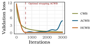
Figure 1: Exemplary course of the empirical risk for different CWB variations on a test data. The red dashed line indicates the optimal stopping iteration found by ACWB. All three methods are trained for 3000 iterations.

The example shown in Figure 1 depicts the behavior of our proposed adaption. After early stopping ACWB, we can continue to further decrease the validation error, whereas continuing training with acceleration (ACWB) increases the validation error. Fine-tuning ACWB thus improves the performance of ACWB while requiring less iterations compared to CWB with a similar validation error. In Section 4.1, we investigate computational advantages of the hybrid approach in terms of runtime, memory consumption, and estimation properties.

4 Experiments

We study the efficacy of the proposed improvements on simulated and real-world data (cf. Appendix B.2). All CWB variants (CWB, ACWB, and HCWB) are either denoted with (nb) if no binning is applied, or (b) if binning is used. The hyperparameters (HPs) of our proposed algorithm are the amount of binning, the momentum rate $\gamma$, and the patience parameter $pat_{0}.$ Further HPs for all CWB variants (including vanilla CWB) are the learning rate $\nu$, the degrees of freedom df, and the number of boosting iterations $M$. As simulation studies and real-world applications have different purposes, we will define separate HP tuning schemes for both but set the number of bins to $n^{\ast}=2$, as suggested by Wood et al. (2017), and the patience parameter to $pat_{0}=5$ for all experiments. HPs defining the flexibility of base learners such as number of knots or the degree of basis functions for P-Spline base learners are set to 20 knots and degree 3, respectively.

In Section 4.1, we first use simulated data to investigate the following hypotheses:

• (memory and runtime efficiency of binning): Compared to CWB (nb), binning reduces memory consumption and runtime.

• (partial effects of binning): Compared to CWB (nb), using CWB (b) does not deteriorate the estimation quality of partial effects.

• (iterations and partial effects of accelerated methods): Compared to CWB (nb), ACWB (nb) and HCWB (nb) require fewer iterations to achieve almost identical partial effect estimates.

• (scaling behaviour of ACWB/HCWB): Empirical runtimes of binning and ACWB follow the previously derived complexity conditions and thus scale efficiently with an increasing number of observations and base learners.

In addition to the simulation study, we conduct a comparison of CWB and HCWB on real-world data sets in Section 4.2. Here, we investigate the following experimental questions:

• (implementation comparison with the state-of-the-art software mboost): Compared to mboost, our implementation compboost is less time-consuming during model training.

• (algorithmic comparison of accelerated methods): When compared to vanilla CWB (nb), the prediction performance of the five proposed CWB variants (CWB (b), ACWB/HCWB (b)/(nb)) does not deteriorate while yielding faster runtimes.

• (comparison with state-of-the-art algorithms) The prediction performance of ACWB (b) and HCWB (b) is competitive with state-of-the-art boosting algorithms while yielding notably faster runtimes.

All simulations and benchmarks are conducted using R (R Core Team, 2021) version 3.6.3 on three identical servers with 32 2.60 GHz Intel(R) Xeon(R) CPU e5-2650 v2 processors. Reproducibility of benchmark and simulation results is ensured by providing a Docker image with pre-installed software and benchmark code. References to GitHub repositories containing our compboost software and the raw benchmark source code with results are referenced in the Supplementary Material.

4.1 Numerical Experiments on Simulated Data

4.1.1 Simulation Setup

We define the number of informative and noise features as $p$ and $p_{\text{noise}}$, respectively. Numerical features $\mathbf{x}_{j}$ are simulated by drawing the minimum value $x_{j,\text{min}}$ from a uniform distribution $U[0,100]$ and the maximal value $x_{j,\text{max}}=x_{j,\text{min}}+\rho_{k}$, where $\rho_{k}$ also follows a uniform distribution $U[0,100]$. The $n$ feature values $\mathbf{x}_{j}$ are simulated i.i.d. from $U[x_{j,\text{min}},x_{j,\text{max}}]$. All feature effects are simulated as non-linear effects using splines. The spline basis $\bm{Z}_{k}$ for the simulation is created using feature $\mathbf{x}_{j}$ with splines of order 4 and 10 inner knots. To obtain unique splines for each $\mathbf{x}_{j}$, we sample $\tau_{k}\sim\mathcal{N}_{10}(0,9)$ and define the $j$th feature effect as $\bm{\eta}_{k}=\bm{Z}_{k}\bm{\tau}_{k}$. Each of the $p_{\text{noise}}$ noise features $\dot{\bm{x}}_{j}$ are drawn from a standard normal distribution. The final data set is given as $\mathcal{D}=\{(x_{1}^{(i)},\dots,x_{p}^{(i)},\dot{x}_{1}^{(1)},\dots,\dot{x}_{p_{\text{noise}}}^{(i)},y^{(i)})\ |\ i=1,\dots,n\}$ with target vector $\bm{y}\sim\mathcal{N}_{n}(\bm{\eta},\mathop{\sf diag}_{n}{(\hat{\sigma}^{2}(\bm{\eta})/\text{SNR}^{2}}))$, where SNR is the signal-to-noise ratio, $\bm{\eta}=\sum_{j=1}^{p}\bm{\eta}_{k}$ and $\hat{\sigma}(\bm{\eta})$ the sample variance of $\bm{\eta}$. Different values of SNR can be used to test CWB on regression tasks of varying hardness.

The experimental design is defined on a grid with $n\in\{5000,10000,20000,50000,100000\}$, $p\in\{5,10,20,50\}$, $p_{\text{noise,rel}}\in\{0.5,1,2,5\}$ with $p_{\text{noise}}=p\cdot p_{\text{noise,rel}}$, and $\text{SNR}\in\{0.1,1,10\}$. The choices of $n$, $p$, and $p_{\text{noise}}$ are particularly relevant for memory and runtime investigations (H1) and (H4). For each combination of experimental settings, we draw 20 different target vectors for statistical replications of each scenario. When measuring the memory consumption, we only use one statistical replication of each configuration, as the memory consumption is almost identical for all repetitions of one configuration. We use valgrind (Nethercote and Seward, 2007) to measure the allocated memory. For memory and runtime comparisons and thus also for complexity considerations, the number of boosting iterations is set to 200. In order to assess the estimation performance of partial effects (H2) and (H3), we use the mean integrated squared error $\text{MISE}=\frac{1}{p}\sum_{j=1}^{p}\int_{\mathop{\sf min}(\mathbf{x}_{j})}^{\mathop{\sf max}(\mathbf{x}_{j})}(b_{k}(x,\bm{\theta}_{k})-b_{k}(x,\hat{\bm{\theta}}_{k}))^{2}dx$ between the estimated base learner $b_{k}(\mathbf{x},\hat{\bm{\theta}}_{k})$ and the true effect $b_{k}(\mathbf{x},\bm{\theta}_{k})$ given by the randomly generated spline.

For performance comparisons, we use CWB with early stopping based on a large, noise-free data set. This ensures correct early stopping and allows us to draw conclusions on CWB’s estimation performance without additional uncertainty induced by finding the optimal stopping iteration. We evaluate different momentum learning rates on a uniform grid from $10^{-1}$ to $10^{-7}$. For CWB as well as for ACWB and HCWB, we set the learning rate to $\nu=0.05$, as suggested in the literature (Bühlmann et al., 2007), and use $\text{df}=5$, which provides just enough flexibility for our simulated non-linear functions. The number of boosting iterations are fixed for H1 and dynamically found for H2 and H3.

4.1.2 Results

H1 (memory and runtime efficiency of binning). Figure 2 illustrates the faster runtime as well as the savings in memory consumption w.r.t. $n$ and $p$. With binning, CWB is four times faster for smaller data sets and up to six times faster for larger data sets. For smaller data sets, binning improves the memory consumption only slightly. Improvements do become large enough to be meaningful when the model is trained on larger data sets and/or more features, consuming only up to a seventh of the original memory usage. Appendix B.4.1 contains an empirical verification of the computational complexity reported in Section 3.1.3 using the results from H1.

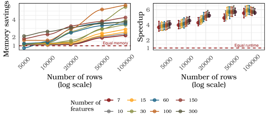
Figure 2: Relative memory savings (left) and speedup as relative runtime (right) when binning is applied compared to no binning (H1). The memory savings and speedup are defined as a ratio of memory or time used by the original algorithm without binning divided by the memory consumption or runtime when binning is applied. The dashed red line indicates an equal memory consumption or runtime of both methods.

H2 (partial effects of binning). The left plot of Figure 3 shows one exemplary comparison of the true effect, the estimated effect using binning, and the estimated effect without binning. The MISE is visualized by the red shaded area between the true and estimated function. As shown on the right in Figure 3, there is no notable difference between the MISE whether binning is applied or not.

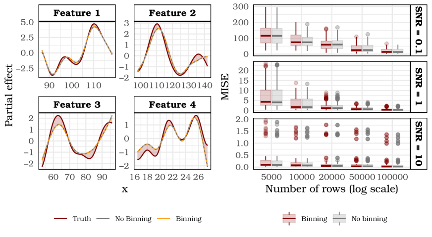
Figure 3: Left: Exemplary estimated partial and true effects for $100000$ observations, $4$ features, and a SNR of $0.1$. The MISE of the curves are $49.08$ for CWB and $49.10$ for CWB with binning. Right: Comparison of the MISE when using binning vs. no binning.

H3 (iterations and partial effects of accelerated methods). Figure 4 (left) shows the difference of MISE values of CWB compared to HCWB and ACWB. As hypothesized, partial effect estimation of ACWB is inferior to CWB due to its acceleration and potentially stopping too early or overshooting the optimal solution. This difference is negligible for small momentum values, but not for higher values. It is worth noting that the SNR in this cases is rather large, potentially undermining the effect of residual-correcting base learners of ACWB. Based on the given results, we recommend a default momentum value of $\gamma=0.0034$ for ACWB, yielding small MISE differences while simultaneously maximizing the speedup. In contrast, HCWB performs as strongly as CWB or even better for settings with more noise (smaller SNR). The right pane of Figure 4 shows the relative ratio of early stopping iterations between CBW and HCWB or ACWB. In almost all cases, the accelerated versions require fewer iterations than CWB. This is especially striking for higher momentum values, and hence we suggest a default of $\gamma=0.037$ for HCWB. In settings with moderate or large SNR, HCWB requires as many iterations as CWB.

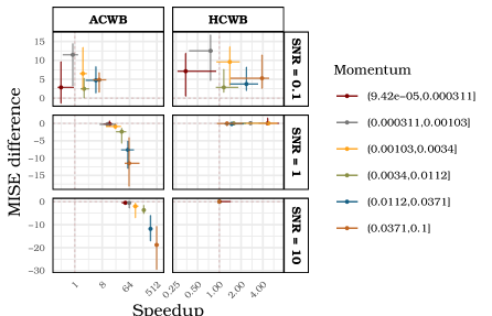
Figure 4: Left: MISE difference between CWB and ACWB/HCWB for partial effect estimation for different momentum values (colors) and SNR (rows). A negative difference indicates that CWB has a lower MISE and therefore a better estimation. Right: Multiplicative factor of iterations needed to train CWB compared to ACWB/HCWB, categorized by the momentum parameter (colors) and SNR (facets). A value of 10 indicates that ACWB/HCWB requires 10 times fewer iterations than CWB until convergence.

H4 (scaling behavior of ACWB/HCWB). Next, we empirically investigate runtimes to scrutinize our derivations in Section 3.1.3 and 3.2.2. To this end, we use the available runtimes, fit a model for each complexity statement to the given data, and compare the estimates to the theoretically derived factors in our complexity analyses. The full results are given in Appendix B.4. In summary, for both binning and ACWB, fitted models yield an (almost) perfect fit with an $R^{2}$ of $1$ and $0.975$, respectively, thus underpinning our complexity estimates with only smaller deviations from theoretical numbers. In particular, this confirms the presumed speedup when using binning and the efficiency of ACWB, scaling linearly in $n$ and $K$.

4.2 Benchmark on Real-World Data

4.2.1 Setup

Algorithms: We compare six CWB variants with XGBoost (Chen et al., 2018) and EBM (Nori et al., 2019). XGBoost represents an efficient and well-performing state-of-the-art implementation of gradient boosting with tree base learners (Friedman and Hastie, 2001). EBM is used to compare against a recent and interpretable boosting method. Like CWB, EBM is based on additive models with additional pairwise interactions, but instead uses a different fitting technique based on a round robin selection of base learners. Although the model can be interpreted by looking at partial effects, some other key features of CWB such as unbiased feature selection cannot be directly transferred to EBM.

Benchmark settings: For performance comparisons in EQ2 and EQ3, we use the area under the ROC curve (AUC) based on a 5-fold cross validation (CV). Additionally, we employ a nested resampling to ensure unbiased performance estimation (Bischl et al., 2012) for EQ3. In the inner loop, models are tuned via Hyperband (Li et al., 2017). We use the number of boosting iterations as a budget parameter for Hyperband. We start at 39 iterations and doubled the iterations until 5000 iterations are reached. This results in 314 different HP configurations for each learner. Each of these HP configuration is evaluated using a 3-fold CV (the inner CV loop). Table 1 lists the used algorithms, the corresponding software packages, and HP spaces from which each HP configuration is sampled.

Used software: All experiments are executed using R (R Core Team, 2021). The packages used for the benchmark are mlr3 (Lang et al., 2019) as a machine learning framework with extensions, including mlr3tuning (Becker et al., 2021) for tuning, mlr3pipelines (Binder et al., 2021) for building pre-processing pipelines such as imputation or feature encoding, and mlr3hyperband (Becker et al., 2021). The package interpret, which implements EBM, was used by calling the Python implementation (Nori et al., 2019) using reticulate (Ushey et al., 2020) to run EBM with its full functionality. The HP space of XGBoost is defined as the “simple set” suggested in Thomas et al. (2018).

Algorithm	Software	Hyperparameter space
CWB/ACWB/HCWB (nb) CWB/ACWB/HCWB (b)	compboost	$\texttt{df}\in[2,10]$ $\texttt{df\_cat}\in[2,10]$ $\texttt{learning\_rate}\in[0.001,0.5]$
XGBoost	xgboost (Chen et al., 2018)	$\texttt{eta}\in[0.001,0.5]$ $\texttt{max\_depth}\in\{1,\dots,20\}$ $\texttt{colsample\_bytree}\in[0.5,1]$ $\texttt{colsample\_bylevel}\in[0.5,1]$ $\texttt{subsample}\in[0.3,1]$ $\texttt{lambda}\in\{2^{\lambda}\ |\ \lambda\in[-10,10]\}$ $\texttt{alpha}\in\{2^{\alpha}\ |\ \alpha\in[-10,10]\}$
EBM	interpret (Nori et al., 2019)	$\texttt{learning\_rate}\in[0.001,0.5\}$

Table 1: Algorithm name, software package, HP space, and number of outer evaluations of all modeling techniques compared in the benchmark.

4.2.2 Results

EQ1 (implementation comparison with the state-of-the-art CWB implementation mboost). A comparison of our vanilla CWB implementation compboost with the state-of-the-art implementation mboost already reveals a speedup of 2 to 4 using compboost. When additionally using acceleration methods and binning, an increase of the speedup up to a factor of 30 for MiniBooNE and Albert can be achieved. As CWB (nb) in compboost and mboost implement the same algorithm, they are equivalent in their predictive performance. Full details are given in Appendix B.6.

EQ2 (algorithmic comparison of accelerated methods). As shown in Figure 5, HCWB (orange) learns faster than CWB (green) due to the acceleration and higher momentum. Performance improvements of ACWB (blue) take longer but surpass CWB on four out of the six data sets. As expected, the AUC of ACWB starts to decrease after the optimal number of boosting iterations is reached, while HCWB corrects this overly aggressive learning behavior by switching to CWB. The runtime of ACWB is about twice as high as for CWB due to the second error-correcting base learner fitted in each iteration (Algorithm 2 line 14). Traces for binning look similar to no binning but do exhibit shorter training times, which underpins the effectiveness of binning.

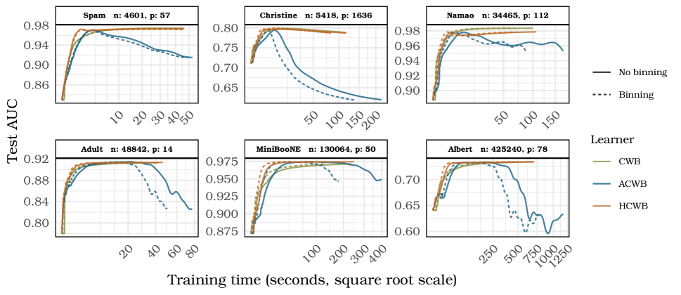
Figure 5: Test AUC traces of all CWB variants over 5000 boosting iterations without early stopping. Each trace is calculated as an average over the 5 runs in the 5-fold CV.

Figure 6 additionally shows test AUC and runtimes of all CWB variants when using early stopping based on a validation data set (defined as 30% of the training data). To check if performance changes between different models are significant, we use the resulting AUC values and compute a beta regression with learners as covariates and the AUC as a response variable (see Appendix B.8). Both ACWB (p-value $=0.4122$) and HCWB (p-value $=0.6927$) do not yield a significantly smaller AUC value. Furthermore, results show that binning does also not have a significant effect on the performance (p-value $=0.9594$). At the same time, binning improves the runtime by an average speedup of 1.5 for all three CWB variants (cf. Appendix B.7 Table 3). ACWB and HCWB even yield further improvements with an average speedup of 3.8 and 2.38, respectively.

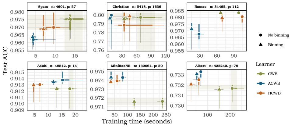
Figure 6: Scatter plot of average AUC values and training times for all CWB variants (color / symbol). Horizontal and vertical boxes indicate the 25- and 75%-quantile, and colored lines indicate the possible range of values. Light green areas additionally highlight the 25- and 75%-quantiles of CWB (nb) to facilitate easy comparison of other CWB variants with this baseline.

EQ3 (comparison with state-of-the-art algorithms). Figure 7 shows that state-of-the-art algorithms benefit from their more complex model structure by also considering complex feature interactions (EBM allows for interactions by design, while XGBoost uses tree base learners, which induce more complex interactions with larger tree depth). The improvement in AUC of these methods compared to CWB is only practically relevant for the data set Christine, which shows an AUC increase of 3.42% for XGBoost. The AUC improvement for all other tasks is (notably) smaller than 3%, even though our approach uses a fully interpretable model. In terms of runtime, ACWB (b) and HCWB (b) outperform XGBoost and EBM on most data sets. On the data sets Spam and Christine, XGBoost is faster than our algorithms, which we attribute to their small sample size. In general, ACWB (b) and HCWB (b) are 4.62 times faster than EBM and 1.66 times faster than XGBoost.

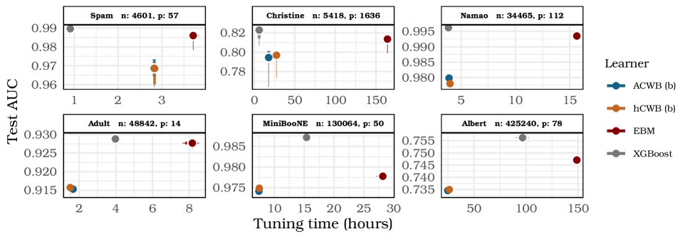
Figure 7: AUC and training time of ACWB (b), HCWB (b), XGBoost, and EBM.

5 Conclusion

Adaptions to CWB presented in this paper can notably improve the use of computational resources, reducing runtimes by up to a factor of 6 and memory usage up to factor of 4, depending on the size of the task. Incorporating binning with equally spaced design points efficiently leverages CWB’s base learner structure with one feature per base learner. Benchmark results show that binning reduces the training time without impairing the predictive performance. The proposed accelerated CWB algorithm (ACWB) is furthermore a natural extension of CWB and provides a faster training procedure at the expense of a potential deterioration of predictive performance when not stopped properly. Our alternative hybrid solution (HCWB) accounts for this and presents no drawbacks in comparison to the standard CWB algorithm. However, HCWB does incur slightly longer runtimes compared to ACWB. In practice, HCBW yields good out-of-the-box performance, while ACWB does not require an additional validation data set and can thus be beneficial in low sample size regimes. Future research will investigate how the proposed framework can be used and further improved for more complex additive models structures in both the predictors as well as in the outcome, e.g., for functional regression models.

ACKNOWLEDGMENT

This work was supported by the German Federal Ministry of Education and Research (BMBF) under Grant No. 01IS18036A and Federal Ministry for Research and Technology (BMFT) under Grant FKZ: 01ZZ1804C (DIFUTURE, MII). The authors of this work take full responsibilities for its content.

SUPPLEMENTARY MATERIAL

Appendix:

Descriptions of possible categorical feature representations with a short comparison w.r.t. runtime and memory consumption as well as class selection properties in the presence of noise. The Appendix further contains empirical validation of the computational complexity estimates as given in Section 2.4 and 3.1.3. Lastly, the appendix contains a figure showing the full benchmark, as well as a generalized linear model to statistically investigate the effect of our adaptions on the predictive performance. (PDF file)

Source code of compboost:

github.com/schalkdaniel/compboost (Commit tag of the snapshot used in this paper: c68e8fb32aea862750991260d243cdca1d3ebd0e)

Benchmark source code:

https://github.com/schalkdaniel/cacb-paper-bmr

Benchmark Docker:

Docker image with pre-installed packages to run the benchmark and access results for manual inspection: hub.docker.com/repository/docker/schalkdaniel/cacb-paper-bmr

References

- Becker et al. (2021) Becker, M., S. Gruber, J. Richter, J. Moosbauer, and B. Bischl (2021). mlr3hyperband: Hyperband for ’mlr3’. R package version 0.1.2.
- Becker et al. (2021) Becker, M., M. Lang, J. Richter, B. Bischl, and D. Schalk (2021). mlr3tuning: Tuning for ’mlr3’. R package version 0.8.0.
- Binder et al. (2021) Binder, M., F. Pfisterer, L. Schneider, B. Bischl, M. Lang, and S. Dandl (2021). mlr3pipelines: Preprocessing Operators and Pipelines for ’mlr3’. R package version 0.3.4.
- Bischl et al. (2012) Bischl, B., O. Mersmann, H. Trautmann, and C. Weihs (2012). Resampling methods for meta-model validation with recommendations for evolutionary computation. Evolutionary computation 20(2), 249–275.
- Brockhaus et al. (2020) Brockhaus, S., D. Rügamer, and S. Greven (2020). Boosting functional regression models with fdboost. Journal of Statistical Software 94(10), 1–50.
- Bühlmann et al. (2007) Bühlmann, P., T. Hothorn, et al. (2007). Boosting algorithms: Regularization, prediction and model fitting. Statistical science 22(4), 477–505.
- Bühlmann and Yu (2003) Bühlmann, P. and B. Yu (2003). Boosting with the L2 loss: regression and classification. Journal of the American Statistical Association 98(462), 324–339.
- Chen and Guestrin (2016) Chen, T. and C. Guestrin (2016). Xgboost: A scalable tree boosting system. In Proceedings of the 22nd acm sigkdd international conference on knowledge discovery and data mining, pp. 785–794.
- Chen et al. (2018) Chen, T., T. He, M. Benesty, V. Khotilovich, and Y. Tang (2018). xgboost: Extreme Gradient Boosting. R package version 0.6.4.1.
- Duff et al. (1989) Duff, I. S., R. G. Grimes, and J. G. Lewis (1989). Sparse matrix test problems. ACM Transactions on Mathematical Software (TOMS) 15(1), 1–14.
- Eilers and Marx (1996) Eilers, P. H. and B. D. Marx (1996). Flexible smoothing with B-splines and penalties. Statistical science, 89–102.
- Freund et al. (1996) Freund, Y., R. E. Schapire, et al. (1996). Experiments with a new boosting algorithm. In icml, Volume 96, pp. 148–156. Citeseer.
- Friedman and Hastie (2001) Friedman, J. and T. Hastie (2001). Greedy function approximation: a gradient boosting machine. Annals of Statistics, 1189–1232.
- Grove and Schuurmans (1998) Grove, A. J. and D. Schuurmans (1998). Boosting in the limit: Maximizing the margin of learned ensembles. In AAAI/IAAI, pp. 692–699.
- Hofner et al. (2011) Hofner, B., T. Hothorn, T. Kneib, and M. Schmid (2011). A framework for unbiased model selection based on boosting. Journal of Computational and Graphical Statistics 20(4), 956–971.
- Hofner et al. (2016) Hofner, B., A. Mayr, and M. Schmid (2016). gamboostLSS: An R package for model building and variable selection in the GAMLSS framework. Journal of Statistical Software 74(1).
- Hothorn et al. (2020) Hothorn, T., P. Buehlmann, T. Kneib, M. Schmid, and B. Hofner (2020). mboost: Model-based boosting. R package version 2.9-2.
- Jiang et al. (2004) Jiang, W. et al. (2004). Process consistency for adaboost. The Annals of Statistics 32(1), 13–29.
- Lang et al. (2019) Lang, M., M. Binder, J. Richter, P. Schratz, F. Pfisterer, S. Coors, Q. Au, G. Casalicchio, L. Kotthoff, and B. Bischl (2019). mlr3: A modern object-oriented machine learning framework in R. Journal of Open Source Software.
- Lang et al. (2014) Lang, S., N. Umlauf, P. Wechselberger, K. Harttgen, and T. Kneib (2014). Multilevel structured additive regression. Statistics and Computing 24(2), 223–238.
- Li et al. (2017) Li, L., K. Jamieson, G. DeSalvo, A. Rostamizadeh, and A. Talwalkar (2017). Hyperband: A novel bandit-based approach to hyperparameter optimization. The Journal of Machine Learning Research 18(1), 6765–6816.
- Li and Wood (2020) Li, Z. and S. N. Wood (2020). Faster model matrix crossproducts for large generalized linear models with discretized covariates. Statistics and Computing 30(1), 19–25.
- Liew et al. (2020) Liew, B. X., D. Rugamer, A. Stocker, and A. M. De Nunzio (2020). Classifying neck pain status using scalar and functional biomechanical variables – Development of a method using functional data boosting. Gait & posture 76, 146–150.
- Lu et al. (2020) Lu, H., S. P. Karimireddy, N. Ponomareva, and V. Mirrokni (2020). Accelerating Gradient Boosting Machines. In International Conference on Artificial Intelligence and Statistics, pp. 516–526.
- Molnar (2020) Molnar, C. (2020). Interpretable Machine Learning. Lulu.com.
- Nesterov (1983) Nesterov, Y. (1983). A method for solving the convex programming problem with convergence rate .
- Nethercote and Seward (2007) Nethercote, N. and J. Seward (2007). Valgrind: a framework for heavyweight dynamic binary instrumentation. ACM Sigplan notices 42(6), 89–100.
- Nori et al. (2019) Nori, H., S. Jenkins, P. Koch, and R. Caruana (2019). Interpretml: A unified framework for machine learning interpretability. arXiv preprint arXiv:1909.09223.
- Qian (1999) Qian, N. (1999). On the momentum term in gradient descent learning algorithms. Neural networks 12(1), 145–151.
- R Core Team (2021) R Core Team (2021). R: A Language and Environment for Statistical Computing. Vienna, Austria: R Foundation for Statistical Computing.
- Ruder (2016) Ruder, S. (2016). An overview of gradient descent optimization algorithms. arXiv preprint arXiv:1609.04747.
- Rügamer et al. (2018) Rügamer, D., S. Brockhaus, K. Gentsch, K. Scherer, and S. Greven (2018). Boosting factor-specific functional historical models for the detection of synchronization in bioelectrical signals. Journal of the Royal Statistical Society: Series C (Applied Statistics) 67(3), 621–642.
- Rügamer and Greven (2020) Rügamer, D. and S. Greven (2020). Inference for L2-Boosting. Statistics and Computing 30, 279–289.
- Saintigny et al. (2011) Saintigny, P., L. Zhang, Y.-H. Fan, A. K. El-Naggar, V. A. Papadimitrakopoulou, L. Feng, J. J. Lee, E. S. Kim, W. K. Hong, and L. Mao (2011). Gene expression profiling predicts the development of oral cancer. Cancer Prevention Research 4(2), 218–229.
- Schalk et al. (2018) Schalk, D., J. Thomas, and B. Bischl (2018). compboost: Modular Framework for Component-wise Boosting. Journal of Open Source Software 3(30), 967.
- Thomas et al. (2018) Thomas, J., S. Coors, and B. Bischl (2018). Automatic gradient boosting. In International Workshop on Automatic Machine Learning at ICML.
- Thomas et al. (2017) Thomas, J., T. Hepp, A. Mayr, and B. Bischl (2017). Probing for sparse and fast variable selection with model-based boosting. Computational and mathematical methods in medicine 2017.
- Ushey et al. (2020) Ushey, K., J. Allaire, and Y. Tang (2020). reticulate: Interface to ’Python’. R package version 1.18.
- Wang et al. (2020) Wang, B., T. M. Nguyen, A. L. Bertozzi, R. G. Baraniuk, and S. J. Osher (2020). Scheduled restart momentum for accelerated stochastic gradient descent. arXiv preprint arXiv:2002.10583.
- Wood et al. (2017) Wood, S. N., Z. Li, G. Shaddick, and N. H. Augustin (2017). Generalized additive models for gigadata: modeling the UK black smoke network daily data. Journal of the American Statistical Association 112(519), 1199–1210.