Complex-valued deep learning with differential privacy

Abstract

We present $\zeta$-DP, an extension of differential privacy (DP) to complex-valued functions. After introducing the complex Gaussian mechanism, whose properties we characterise in terms of $(\varepsilon,\delta)$-DP and Rényi-DP, we present $\zeta$-DP stochastic gradient descent ($\zeta$-DP-SGD), a variant of DP-SGD for training complex-valued neural networks. We experimentally evaluate $\zeta$-DP-SGD on three complex-valued tasks, i.e. electrocardiogram classification, speech classification and magnetic resonance imaging (MRI) reconstruction. Moreover, we provide $\zeta$-DP-SGD benchmarks for a large variety of complex-valued activation functions and on a complex-valued variant of the MNIST dataset. Our experiments demonstrate that DP training of complex-valued neural networks is possible with rigorous privacy guarantees and excellent utility.

1 Introduction

The ability to harness diverse, feature-rich datasets for algorithm training can allow the scientific community to create machine learning (ML) models capable of solving challenging data-driven tasks. These include the creation of robust autonomous vehicles (Rao & Frtunikj, 2018), early-stage cancer discovery (Cruz & Wishart, 2006) or disease survival prediction (Rau et al., 2018). A subclass of these ML problems is able to profit particularly from the ability to execute deep learning workflows over complex-valued datasets, such as magnetic resonance imaging (MRI) (Virtue et al., 2017) or time-series data (Fan & Xiong, 2013; Kociuba & Rowe, 2016). Complex-valued deep learning has seen increased traction in the past years, owing in part to the improved support by ML frameworks and the broader availability of graphics processing unit (GPU) hardware able to tackle the increased computational requirements (Bassey et al., 2021). However, since complex numbers are often used to represent signals derived from sensitive biological or medical records (Cole et al., 2020; Küstner et al., 2020; Peker, 2016), privacy constraints can render such datasets hard to obtain. The resulting data scarcity impairs effective model training, prompting the adoption of regulation-compliant and privacy-preserving methods for data access. Distributed computation methods such as federated learning (FL) (Konečný et al., 2016) can partially address this requirement by only requiring participants to share results of the local computation rather than exchange data over the network. However, FL on its own has repeatedly been shown to be insufficient in the task of privacy protection (Geiping et al., 2020; Yin et al., 2021). Thus, bridging the gap between data protection and utilisation for algorithmic training requires methods able to offer objective privacy guarantees. Differential privacy (DP) (Dwork et al., 2014) has established itself as the cornerstone of such techniques and has been deployed in contexts like the US Census (Abowd, 2018) and distributed learning on mobile devices (Cormode et al., 2018). DP’s purview has been expanded to encompass deep learning through the introduction of DP stochastic gradient descent (DP-SGD) (Abadi et al., 2016), allowing for the training of deep neural networks on private data. So far, however, the application of DP to complex-valued ML tasks remains drastically under-explored. Our work attempts to address this challenge through the following contributions:

1. We extend DP to the complex domain through a collection of techniques we refer to as $\zeta$-DP. We use this term instead of complex-valued DP for brevity and to avoid confusion with the abbreviation cDP, which is already used for concentrated DP (Dwork & Rothblum, 2016). The letter $\zeta$ alludes to the complex-valued Riemann $\zeta$ function and is intended to convey the notion of continuation to the complex domain.

2. We define and discuss the complex Gaussian Mechanism (GM) in Section 4.1 and show that its properties generalise corresponding results on real-valued functions. This allows us to interpret the complex GM through the lens of previous work on $(\varepsilon,\delta)$-DP and Rényi-DP (RDP).

3. To enable the design and privacy-preserving training of complex-valued deep learning models, we introduce $\zeta$-DP-SGD in Section 4.2.

4. Finally, in Section 5 we experimentally evaluate our techniques on several real-life neural network training tasks, i.e. speech classification, abnormality detection in electrocardiograms and magnetic resonance imaging (MRI) reconstruction. Moreover, we establish baselines for future work by providing benchmark results on a complex-valued variant of the MNIST dataset and on complex neural network activation functions both with and without $\zeta$-DP-SGD.

2 Related work

Prior work has addressed several challenges in non-private complex-valued deep learning, including the introduction of appropriate activation functions, and has presented applications in domains such as MRI reconstruction (Küstner et al., 2020) or time series analysis (Fink et al., 2014). For a detailed overview of methodology and applications, we refer to Hirose (2012); Bassey et al. (2021). Until recently, deep learning frameworks did not fully support complex arithmetic and automatic differentiation. Hence, previous works (Trabelsi et al., 2017; Nazarov & Burnaev, 2020) express $\mathbb{C}$ as $\mathbb{R}^{2}$ and use two real-valued channels rather than complex floating-point numbers. This approach can lead to a spurious increase in function sensitivity and, by extension, to the addition of excessive noise in the private setting, adversely impacting utility. Our work specifically addresses this shortcoming through the use of Wirtinger/$\mathbb{CR}$-calculus (Wirtinger, 1927; Kreutz-Delgado, 2009). A limited number of studies have utilised DP techniques in conjunction with complex-valued data (Fan & Xiong, 2013; Fioretto et al., 2019), however, to our knowledge none has formalised a notion of complex-valued DP or investigated neural network applications. The $(\varepsilon,\delta)$-definition of DP and the Gaussian mechanism are essential to our formalism, and details on their real-valued definitions can be found in Dwork et al. (2014). As stated above, DP-SGD was introduced by Abadi et al. (2016). Rényi-DP (RDP) was introduced by Mironov (2017) as a relaxation of $(\varepsilon,\delta)$-DP with favourable properties under composition, rendering it particularly useful for DP-SGD privacy accounting.

3 Background

We begin by introducing key terminology required in the rest of our work. We assume that a trusted analyst in possession of sensitive data wishes to publish the results of some analysis performed on this data while offering the individuals to whom the data belongs a DP guarantee. We will refer to the set of all sensitive records as the sensitive database $D$, whereby we assume that one individual’s data is only present in the database once. Let $X$, the metric space of all sensitive databases, be equipped with the Hamming metric $d_{X}$ and let $D\in X$. $D$’s adjacent database $D^{\prime}$ can be constructed from $D$ by adding or removing exactly one database row (that is, one individual’s data), such that $d_{X}(D,D^{\prime})=1$. The analyst executes a query (function) $f$, for example a mean calculation, over the database. We first define the sensitivity of $f$:

Definition 1 (Sensitivity $\Delta$ of $f$).

Let $X$ and $d_{X}$ be defined as above. $f$ maps the elements of $X$ to elements of a metric space $Y$ equipped with a metric $d_{Y}$. The (global) sensitivity $\Delta$ of $f$ is then defined as:

$$\Delta(f)=\max_{D,D^{\prime}\in X}\frac{d_{Y}(f(D),f(D^{\prime}))}{d_{X}(D,D^{\prime})},D\neq D^{\prime}.$$ (1)

The maximum is taken over all adjacent database pairs in $X$. When $Y$ is the Euclidean space and $d_{Y}$ is the $L_{2}$ metric, $\Delta$ is referred to as the $L_{2}$ sensitivity. We will only use the $L_{2}$ sensitivity in this work.

In private data analysis and ML, we are often concerned with differentiable functions; for Lipschitz-continuous query functions, the equivalence of the Lipschitz constant and the $L_{2}$-sensitivity (Raskhodnikova & Smith, 2016) can be exploited:

Definition 2 (Lipschitz constant $K$ of $f$).

Let $X,Y,d_{X}$ and $d_{Y}$ be defined as above. Then $f$ is said to be $K$-Lipschitz continuous if and only if a non-negative real number $K_{f}$ exists for which the following holds:

$$d_{Y}(f(D),f(D^{\prime}))\leq K_{f}\,d_{X}(D,D^{\prime}).$$ (2)

Evidently, $K_{f}\equiv\Delta$ by Equation (1) and the definition of adjacency. Moreover, let $\mathcal{D}$ be the differential operator; then $K_{f}=\sup\|\mathcal{D}(f)\|$, where $\|\cdot\|$ is the operator norm (O’Searcoid, 2006). Therefore, for a scalar-valued query function, $\Delta\equiv K_{f}\equiv\sup\|\nabla f\|_{2}$.

A DP mechanism adds noise to the results of $f$ calibrated to its sensitivity. Here, we provide the definition of the (real-valued) Gaussian mechanism (GM):

Definition 3 (Gaussian mechanism).

The Gaussian mechanism $\mathcal{M}$ operates on the results of a query function $f:\mathbb{R}^{n}\mapsto\mathbb{R}^{d}$ with sensitivity $\Delta$ over a sensitive database $D$ by outputting $f(D)+\xi$, where $\xi\sim\mathcal{N}(0,\sigma^{2}\,\mathbf{I}_{d})$. Here, $\mathbf{I}_{d}$ denotes the identity matrix with $d$ diagonal elements and $\sigma^{2}$ is the variance of Gaussian noise calibrated to $\Delta$.

The application of the GM with properly calibrated noise satisfies $(\varepsilon,\delta)$-DP:

Definition 4 ($(\varepsilon,\delta)$-DP).

The randomised mechanism $\mathcal{M}$ preserves $(\epsilon,\delta)$-DP if, for all pairs of inputs $D$ and $D^{\prime}$ and all subsets $\mathcal{S}$ of $\mathcal{M}$’s range:

$$\mathbb{P}(\mathcal{M}(f(D)\in\mathcal{S}))\leq e^{\varepsilon}\,\mathbb{P}(\mathcal{M}(f(D^{\prime})\in\mathcal{S}))+\delta.$$ (3)

A number of relaxations have been proposed to characterise the properties of the GM, of which Rényi DP is arguably the most widely employed in DP deep learning frameworks owing to its favourable properties under composition.

Definition 5 (Rényi DP).

$M$ preserves $(\alpha,\rho)$-Rényi-DP (RDP) if, for all pairs of inputs $D$ and $D^{\prime}$:

$$D_{\alpha}\left(\mathcal{M}(f(D))\parallel\mathcal{M}(f(D^{\prime}))\right)\leq\rho$$ (4)

where $D_{\alpha}$ denotes the Rényi divergence of order $\alpha>1$.

4 $\zeta$-DP

In this section we introduce $\zeta$-DP, an extension of DP to complex-valued query functions and mechanisms. $\zeta$-DP generalises real-valued DP and allows the re-use of prior theoretical results and software implementations.

4.1 The complex Gaussian mechanism

We begin by introducing a variant of the GM suitable to query functions with codomain $\mathbb{C}$.

Definition 6 (Complex Gaussian mechanism).

The complex Gaussian mechanism $\mathcal{M_{\mathbb{C}}}$ on $f:\mathbb{C}^{n}\mapsto\mathbb{C}^{d}$ outputs $f(D)+\xi$, where $\xi\sim\mathcal{N}_{\mathbb{C}}(0,\sigma^{2}\,\mathbf{I}_{d})$ and $\mathcal{N}_{\mathbb{C}}(0,\sigma^{2})$ denotes circularly symmetric complex-valued Gaussian noise with variance $\sigma^{2}$.

Of note, a random variable $X\sim\mathcal{N}_{\mathbb{C}}(0,\sigma^{2})$ can be constructed by independently drawing two random variables $A,B$ from a real-valued normal distribution $\mathcal{N}(0,\frac{\sigma^{2}}{2})$ and outputting $X=A+B\,\bm{\mathrm{i}}$, where $\,\bm{\mathrm{i}}$ is the imaginary unit.

We now state our two main theoretical results:

Theorem 1.

Let $f:\mathbb{C}^{n}\mapsto\mathbb{C}^{d}$ be a query function with sensitivity $\Delta$. Then, $\mathcal{M_{\mathbb{C}}}$ preserves $(\varepsilon,\delta(\varepsilon))$-DP if and only if the following holds $\forall\,\varepsilon>0,\delta\in[0,1]$:

$$\delta(\varepsilon)\geq\Phi\left(\frac{\Delta}{2\sigma}-\frac{\varepsilon\sigma}{\Delta}\right)-e^{\varepsilon}\Phi\left(-\frac{\Delta}{2\sigma}-\frac{\varepsilon\sigma}{\Delta}\right)$$ (5)

where $\Phi$ denotes the cumulative distribution function of the standard (real-valued) normal distribution.

Proof.

The claim represents a generalisation of the Analytic Gaussian Mechanism (Balle & Wang, 2018) to $\mathcal{M_{\mathbb{C}}}$. It suffices to show that the magnitude of the privacy-loss random variable $\Omega$ is bounded by $\varepsilon$ with probability $1-\delta$. As shown in Dwork & Rothblum (2016) and Balle & Wang (2018), given some fixed output $O\in\mathbb{C}^{d}$, $\Omega$ is given by:

$$\Omega=\log\left(\frac{\mathbb{P}(\mathcal{M}_{\mathbb{C}}(f(D))=O)}{\mathbb{P}(\mathcal{M}_{\mathbb{C}}(f(D^{\prime}))=O)}\right)$$ (6)

where $\log$ is the natural logarithm, and is distributed as:

$$\mathcal{N}\left(\frac{\|f(D)-f(D^{\prime})\|^{2}_{2}}{2\sigma^{2}},\frac{\|f(D)-f(D^{\prime})\|^{2}_{2}}{\sigma^{2}}\right).$$ (7)

As $\|f(D)-f(D^{\prime})\|^{2}_{2}=(f(D)-f(D^{\prime}))(f(D)-f(D^{\prime}))^{H}\in\mathbb{R}$, where $H$ denotes the Hermitian transpose, $\Omega$ has a real-valued mean and hence follows a real-valued normal distribution, even when $O\in\mathbb{C}$. From here, the proof proceeds identically to the proof to Theorem 8 of (Balle & Wang, 2018). ∎

Theorem 2.

Let $f$ be defined as above. Then, $\mathcal{M_{\mathbb{C}}}$ preserves $(\alpha,\rho)$-RDP if:

$$\sigma^{2}\geq\frac{1}{2}\frac{\alpha\Delta^{2}}{\rho}.$$ (8)

We will rely on the following fact about the Rényi divergence of order $\alpha$ between arbitrary distributions:

Corollary 1 (Definition 2 in (Van Erven & Harremos, 2014)).

Let $P$ and $Q$ be two arbitrary distributions defined on a measurable space $(\mathcal{X},\mathcal{F})$ with densities $p(x)$ and $q(x)$. Then, for $\alpha>1$:

$$D_{\alpha}(P\parallel Q)=\frac{1}{\alpha-1}\log\int_{-\infty}^{\infty}p(x)^{\alpha}q(x)^{1-\alpha}\mathrm{d}x.$$ (9)

In particular, for two normal distributions with means $\bm{\mu}_{0}$ and $\bm{\mu}_{1}$ and common variance $\sigma^{2}\mathbf{I}$:

$$D_{\alpha}\left(\mathcal{N}(\bm{\mu}_{0},\sigma^{2}\mathbf{I})\parallel\mathcal{N}(\bm{\mu}_{1},\sigma^{2}\mathbf{I})\right)=\frac{\alpha\,\langle\bm{\mu}_{0},\bm{\mu}_{1}\rangle}{2\sigma^{2}}$$ (10)

where $\langle\cdot\rangle$ denotes the inner product.

We can now prove Theorem 8:

Proof.

By Definition 6 and the additive property of the Gaussian distribution, the density functions of $\mathcal{M_{\mathbb{C}}}$ on $f(D)$ and $f(D^{\prime})$ follow a circularly symmetric complex-valued Gaussian distribution with means $f(D)$ and $f(D^{\prime})$ and common covariance matrix $\sigma^{2}\mathbf{I}$. By substituting in equation (10):

$$D_{\alpha}\left(\mathcal{N}_{\mathbb{C}}(f(D),\sigma^{2})\parallel\mathcal{N}_{\mathbb{C}}(f(D^{\prime}),\sigma^{2})\right)=\frac{\alpha\,\langle f(D),f(D^{\prime})\rangle}{2\sigma^{2}}=$$

$$=\frac{\alpha(f(D)-f(D^{\prime}))(f(D)-f(D^{\prime}))^{H}}{2\sigma^{2}}=\frac{\alpha\|f(D)-f(D^{\prime})\|_{2}^{2}}{2\sigma^{2}}\leq\frac{\alpha\Delta^{2}}{2\sigma^{2}}.$$ (11)

Hence, to preserve $(\alpha,\rho)$-RDP, it suffices to choose $\sigma^{2}$ such that

$$\sigma^{2}\geq\frac{1}{2}\frac{\alpha\Delta^{2}}{\rho}.$$ (12)

∎

These findings allow for a seamless transfer of results which apply to real-valued functions to the complex domain. In particular, they yield the following insights:

1. The complex GM inherits all properties of the $(\varepsilon,\delta)$ and RDP interpretations of the real-valued GM, such as composition and sub-sampling amplification.

2. The complex GM, like the real-valued GM, is fully characterised by the sensitivity $\Delta$ and the magnitude of the noise $\sigma$.

3. The GM naturally fits $\zeta$-DP due to the convenient properties of the circularly symmetric complex-valued Gaussian distribution. As a counterexample, a complex-valued Laplace random variable is naturally non-circular in the complex (and multivariate) case, even when constructed from independent distributions (Kotz et al., 2001). Moreover, the utilisation of the $L_{1}$-metric on the output space of $f$ is disadvantageous, as even for scalar (complex) outputs, the $L_{1}$ sensitivity can be higher than the $L_{2}$ sensitivity. Lastly, the utilisation of elliptical noise is inherently unable to satisfy $(\varepsilon,0)$-DP in any dimension $>1$ (Reimherr & Awan, 2019). We thus leave the introduction of alternative strategies for obtaining $(\varepsilon,0)$-DP in the complex-valued setting to future investigation.

We conclude this section by introducing a modification of the DP stochastic gradient descent (DP-SGD) algorithm, which will be employed in our experimental evaluation.

4.2 $\zeta$-DP-SGD

The DP-SGD algorithm (Abadi et al., 2016) represents an application of the GM to the training of deep neural networks. Using the terminology above, each training step of the neural network (whose loss function, in this setting, represents the query) leads to the release of a privatised gradient. Evidently, the noise magnitude of the GM must be calibrated to the sensitivity of the loss function. However, most neural network loss functions have a Lipschitz constant which is too high to preserve DP while maintaining acceptable utility (and –generally –the Lipschitz constant of neural networks is NP-hard to compute (Scaman & Virmaux, 2018)). Thus, DP-SGD (Abadi et al., 2016) artificially induces a bounded sensitivity condition by clipping the $L_{2}$-norm of the gradient to a pre-defined value. A real-valued loss function is required for minimisation as the complex plane –contrary to the real number line– does not admit a natural ordering. Our implementation of the algorithm makes use of Wirtinger (or $\mathbb{CR}$-) calculus (Kreutz-Delgado, 2009) for gradient computations similar to previous works on complex-valued deep learning (Virtue et al., 2017; Boeddeker et al., 2017). This technique, discussed in detail Appendix A.1, provides several benefits: It relaxes the requirement for component functions to be holomorphic (that is, differentiable in the complex sense), only requiring them to be individually differentiable with respect to their real and imaginary components (differentiable in the real sense). For holomorphic functions $\mathbb{C}\mapsto\mathbb{C}$, $\mathbb{CR}$-derivatives nevertheless recover the correct derivative definition. Thus, $\mathbb{CR}$-derivatives can also be used to compute the global sensitivity in the $\mathbb{C}\mapsto\mathbb{C}$-case via the Lipschitz constant. More importantly, for functions $\mathbb{C}\mapsto\mathbb{R}$, they lead to a correct gradient magnitude calculation, whereas expressing complex-valued functions as vector-valued functions in $\mathbb{R}^{2n}$, a technique often employed in complex-valued neural network training (Trabelsi et al., 2017), can incur an undesirable multiplicative sensitivity increase which would diminish the utility of $\zeta$-DP-SGD. We exemplify this phenomenon and the noise savings $\mathbb{CR}$-calculus can enable in Appendix A.1. $\zeta$-DP-SGD is presented in Algorithm 1 and relies on a modification of the gradient clipping step: we clip the conjugate gradient, which represents the direction of steepest ascent for a real-valued loss function $\mathcal{L}$:

$$\nabla\overline{\mathcal{L}}\coloneqq\left(\frac{\partial\mathcal{L}}{\partial\overline{\theta}_{1}},\dots,\frac{\partial\mathcal{L}}{\partial\overline{\theta}_{n}}\right)$$ (13)

where $\left(\overline{\theta}_{1},\dots,\overline{\theta}_{n}\right)$ is the conjugate weight vector.

Algorithm 1 $\zeta$-DP-SGD

0:  Database with samples $\{x_{1},\ldots,x_{N}\}\in\mathbb{C}^{n}$, neural network with loss function $\mathcal{L}$ and weight vector $\bm{\theta}\in\mathbb{C}^{n}$. Hyperparameters: learning rate $\eta_{t}$, noise variance $\sigma^{2}$, sampling probability $R$, gradient norm bound $B$, total steps $T$.

  Initialize $\bm{\theta}_{0}$ randomly

  for $t\in[T]$ do

     Draw a lot $L_{t}$ with sampling probability $R$ using Poisson or uniform sampling

     Compute per-sample conjugate gradient

     For each $i\in L_{t}$, compute $\overline{\bm{g}}_{t}(x_{i})\leftarrow\nabla\overline{\mathcal{L}}(\bm{\theta}_{t},x_{i})$

     Clip conjugate gradient

     $\widecheck{\bm{g}}_{t}(x_{i})\leftarrow\overline{\bm{g}}_{t}(x_{i})/\max\left(1,\frac{\|\overline{\bm{g}}_{t}(x_{i})\|_{2}}{B}\right)$

     Apply the Complex Gaussian Mechanism and average

     $\widetilde{\bm{g}}_{t}\leftarrow\frac{1}{L}\left(\sum_{i}\widecheck{\bm{g}}_{t}(x_{i})+\mathcal{N}_{\mathbb{C}}(0,\sigma^{2}B^{2}\,\mathbf{I}_{L})\right)$

     Descend

      $\bm{\theta}_{t+1}\leftarrow\bm{\theta}_{t}-\eta_{t}\widetilde{\bm{g}}_{t}$

  end for

  Output updated neural network weight vector $\bm{\theta}_{T}$ and compute the privacy cost.

5 Experimental evaluation

Throughout this section, we present results from the experimental evaluation of $\zeta$-DP-SGD. Details on dataset preparation and training can be found in Appendix A.2.

5.1 Benchmarking $\zeta$-DP-SGD on PhaseMNIST

The MNIST dataset (LeCun et al., 2010) is widely used as a benchmark dataset in real-valued DP-SGD literature. As a means of comparison, we thus begin our experimental evaluation with results on an adapted, complex-valued version of MNIST, which we term PhaseMNIST. In brief, for each example of the original MNIST dataset with label $L_{\mathfrak{R}}\in\{0,\dots,9\}$, we obtain the imaginary component by selecting an image with label $L_{\mathfrak{I}}$ such that $L_{\mathfrak{R}}+L_{\mathfrak{I}}=9$ resulting in an input image arrangement $(0,9),(1,8),\dots,(9,0)$. Only the label of the real-valued image is used. The results are summarised in Table 1, where we also provide baselines for real-valued MNIST training on the same architecture (with real-valued weights).

Table 1: Results for PhaseMNIST training in a private ($\zeta$-DP-SGD) and non-private (non-DP) fashion. Results for real-valued MNIST are provided for approximate comparison using the same model architecture (but with real-valued weights) trained with identical settings.

	Accuracy	$\varepsilon$
PhaseMNIST $\zeta$-DP-SGD	$\mathbf{99.0}\%$	$0.53$
MNIST DP-SGD	$95.67\%$	$0.53$
PhaseMNIST non-DP	$\mathbf{99.3}\%$	$\infty$
MNIST non-DP	$97.43\%$	$\infty$

The complex-weighted neural networks reached $99\%$ accuracy with a low privacy budget consumption of $0.53$. We assume this to be due to the increased amount of information provided by the alignment with a second image as well as the higher entropic capacity of the network due to the complex-valued weights. A similar phenomenon was observed by Scardapane et al. (2018).

5.2 Privacy-preserving electrocardiogram abnormality detection on wearable devices

The advent of wearable devices incorporating electrocardiography (ECG) sensors has provided consumers the ability to detect signs of an abnormal heart rhythm. In this section, we demonstrate the utilisation of a small neural network architecture suitable for deployment, e.g. to a mobile device connected to such a biosensor, to be trained on ECG data from the the China Physiological Signal Challenge (CPSC) 2018 challenge dataset (Liu et al., 2018). We selected the task of automated Left Bundle Branch Block (LBBB) detection, formulated as a binary classification task against a normal (sinus) rhythm. This task is clinically relevant, as the sudden appearance of LBBB can herald acute coronary syndrome which requires urgent attention to avert myocardial infarction. As ECG data constitutes personal health information, its protection is mandated both legally and ethically. We utilised $\zeta$-DP-SGD for training a complex-valued neural network on Fourier-transformed ECG acquisitions. We adopt this strategy as it can benefit from two key properties of the Fourier transform: ECG data can contain high-frequency noise which is irrelevant for diagnosis and can be reduced using Fourier filtering. Concurrently, this technique compresses the signal, which can drastically reduce the amount of data transferred. Table 2 shows classification results and Figure 1 shows exemplary source data.

Table 2: Private and non-private training results in the task of ECG abnormality detection.

	ROC-AUC	$\varepsilon$
Non-DP	$92\%$	$\infty$
$\zeta$-DP-SGD	$92\%$	$1.76$

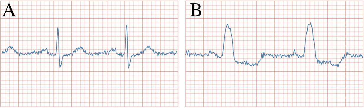
Figure 1: Exemplary ECG data used for classification. A shows an example of a sinus rhythm (normal ECG) and B shows an example of an ECG exhibiting signs of LBBB. Observe also the high frequency noise around the baseline which can be filtered using the Fourier transform.

5.3 Differentially private speech command classification for voice assistant applications

In recent years, voice assistants have gained popularity in consumer applications such as home speakers, and rely heavily on ML. Recordings collected from users for training speech processing algorithms can be used in impersonation attacks, resulting in successful identity theft (Sweet, 2016) or in acoustic attacks, which trigger unintended behaviour in voice assistants (Yuan et al., 2018; Carlini et al., 2016). Protecting privacy in this setting is therefore paramount to increase trust and applicability, as well as safeguard both users and systems from adversarial interference. Convolutional neural networks (CNNs) have been demonstrated to yield state-of-the-art performance on spectrogram-transformed audio data (Palanisamy et al., 2020). However, this and other works (Zhou et al., 2021) typically discard the imaginary components. We here experimentally demonstrate the differentially private training of a 2-dimensional CNN directly on the complex spectrogram data. We utilised a subset of the SpeechCommands dataset (Warden, 2018), specifically samples from the categories Yes, No, Up, Down, Left, Right, On, Off, Stop, and Go, summing up to $8000$ examples. We transformed each waveform signal to a complex-valued 2-D spectrogram and used $\zeta$-DP-SGD to train a complex-valued CNN. These results are summarised in Table 3 and Figure 2.

Table 3: Results on the spectrogram-transformed samples from the SpeechCommands dataset for private and non-private training.

	ROC-AUC	$\varepsilon$
Non-DP	$97.8\%$	$\infty$
$\zeta$-DP-SGD	$92.5\%$	$1.47$

Figure 2: Exemplary waveform (A), real (B) and imaginary (C) spectrogram components from the utterance Stop. Spectrograms are log-magnitude transformed for clarity.

5.4 Benchmarking complex-valued activation functions for $\zeta$-DP-SGD

A number of specialised activation functions, designed for utilisation with complex-valued neural networks, have been proposed in literature. To guide practitioner choice in our newly proposed setting of $\zeta$-DP-SGD training, we here provide activation function benchmarks on the SpeechCommands dataset used in the previous section. Table 4 summarises these results. We consistently found the inverted Gaussian (iGaussian) activation function to perform best in the $\zeta$-DP-SGD setting. This may be in part due to its bounded magnitude, thereby recapitulating the effect Papernot et al. (2020) discuss for real-valued networks, i.e. that bounded activation functions lead to improved performance in DP-SGD. We leave the further investigation of this finding to future work.

Table 4: ROC-AUC (mean$\pm$STD) of complex-valued activation functions on the SpeechCommand dataset trained with identical settings and the same network architecture over five repetitions with $\zeta$-DP-SGD.

Activation function	Reference	ROC-AUC
Separable Sigmoid	Nitta (1997)	$52.9\pm 0.02\%$
zReLU	Guberman (2016)	$54.7\pm 0.03\%$
Trainable Cardioid (per-feature bias)	Virtue et al. (2017)	$80.2\pm 0.02\%$
SigLog	Georgiou & Koutsougeras (1992)	$87.3\pm 0.01\%$
Trainable ModReLU (per-feature bias)	Arjovsky et al. (2016)	$89.0\pm 0.01\%$
Cardioid	Virtue et al. (2017)	$89.2\pm 0.01\%$
Trainable Cardioid (single bias)	Virtue et al. (2017)	$89.4\pm 0.02\%$
ModReLU	Arjovsky et al. (2016)	$89.5\pm 0.01\%$
cReLU	Trabelsi et al. (2017)	$91.9\pm 0.01\%$
iGaussian	Virtue et al. (2017)	$\mathbf{93.4\pm 0.01}\%$

5.5 MRI reconstruction

MRI is an important medical imaging modality and has been studied extensively in the context of deep learning (Akçakaya et al., 2019; Hammernik et al., 2018; Küstner et al., 2020; Muckley et al., 2020). MRI data is acquired in the so-called k-space. Sampling only a subset of k-space data allows for a considerable speed-up in acquisition time, benefiting patient comfort and costs, however, typically leads to image artifacts, which reduce the diagnostic quality of the resulting MR images. Although neural networks have the ability to produce high-quality reconstructions, their usage for this task has been shown to sometimes lead to the appearance of spurious image content from the fully-sampled reference images the models have been originally trained on (Hammernik et al., 2021; Muckley et al., 2020; Shimron et al., 2021). DP could counteract such hallucination as it is designed to limit the effect of individual training examples on model training. However, this positive effect of DP may be counterbalanced by an unacceptable decrease in the diagnostic suitability of the reconstructed images. In this section, we investigate the ramifications of DP on the quality of MRI reconstructions. For this purpose, we trained a complex-valued U-Net model architecture on the task of reconstructing single-coil knee MRI images from the fastMRI dataset (Zbontar et al., 2018) using pseudo-random k-space sampling at $4\times$ acceleration. We observed a nearly equivalent performance in the non-DP and the $\zeta$-DP-SGD settings, whereby the non-DP model enjoyed a $<2\%$ performance advantage in all metrics. Moreover, to assess the diagnostic suitability of the reconstructed images, we asked a diagnostic radiologist who was blinded to whether or not $\zeta$-DP-SGD was used, to compare the resulting scans. No differences in diagnostic suitability were observed by the expert in any of the reconstructed images. We thus conclude that –at least with respect to image quality– DP can indeed match the non-private training of MRI reconstruction models, even at an $\varepsilon$ value of $<1$; we intend to investigate its effect on preventing training data hallucination into reconstructed images in future work. Results from these experiments are summarised in Table 5 and Figure 3.

Table 5: Results on the MRI reconstruction task. NMSE: normalised mean squared error, PSNR: peak signal-to-noise ratio in dB, SSIM: structural similarity index metric.

	NMSE	PSNR	SSIM	$\varepsilon$
Non-DP	$0.042$	$30.74$	$0.70$	$\infty$
$\zeta$-DP-SGD	$0.043$	$30.57$	$0.69$	$0.67$

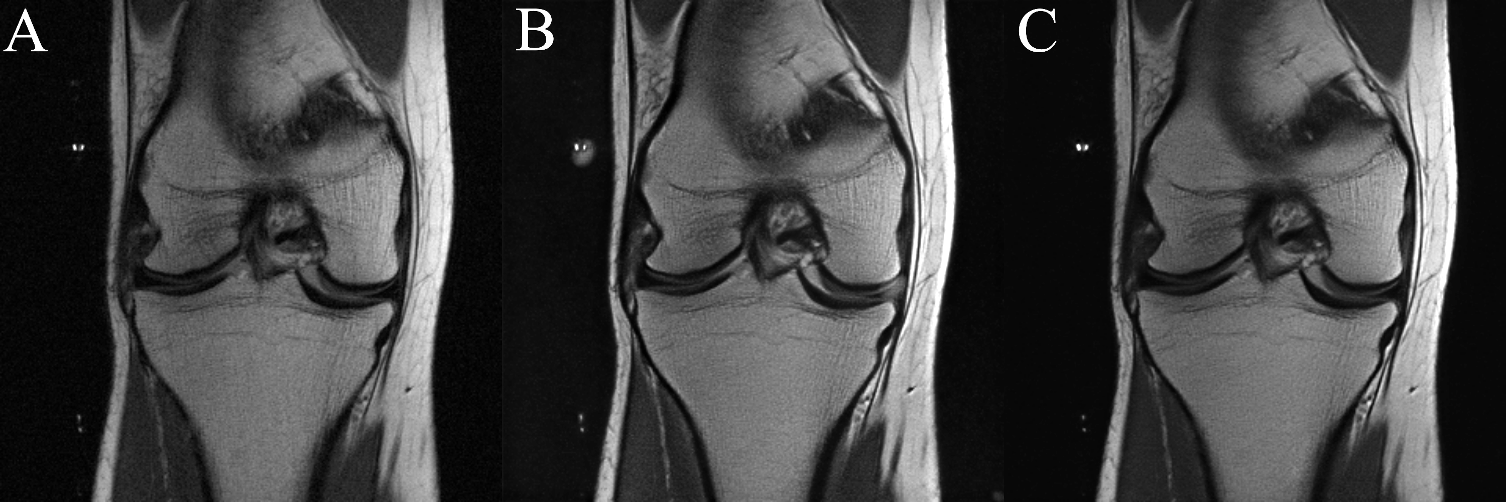
Figure 3: Exemplary reconstruction from a coronal proton-density weighted image of the knee. A: reference image, B: reconstruction model trained non-privately, C: reconstruction model trained with $\zeta$-DP-SGD reconstruction.

6 Conclusion

Our work presents $\zeta$-DP, an extension of DP to the complex domain and introduces key building blocks of DP training, namely the complex Gaussian mechanism and $\zeta$-DP-SGD. Our experiments on real-world tasks demonstrate that the training of DP complex-valued neural networks is possible with high utility under tight privacy guarantees. This may –in part– be attributable to the increased learning capacity of complex-valued models resulting from incorporating two degrees of freedom (real and imaginary) per trainable model parameter. On the flip side, both complex-valued deep learning and DP incur a considerable computational performance penalty. Despite steadily improving complex number support, current deep learning frameworks have not yet implemented a full palette of complex-valued layers and activation functions. Moreover, the software framework utilised to computationally realise $\zeta$-DP-SGD in our work relies on multithreading, which suffers from considerable overhead compared to implementations utilising vector instructions and hardware. We discuss the topic of software implementation and provide computational performance benchmarks in Appendices A.3 and A.4. Our conclusions highlight a requirement for mature software frameworks able to offer feature and performance parity with their real-valued counterparts. We focus on the Gaussian mechanism and the $(\varepsilon,\delta)$-DP/RDP interpretations in this work, believing them to be the most relevant for deep learning applications. The formalisation of other DP mechanisms and interpretations (such as f-DP (Dong et al., 2019)) is a promising future research direction. Such future work could benefit from improved privacy accounting (interestingly also relying on complex numbers, e.g. Zhu et al. (2021)) to diminish –as much as possible– the utility gap to non-private training. In conclusion, we contend that DP and other privacy-enhancing technologies can increase the amount of data available for scientific study, and are optimistic that our work represents a worthwhile contribution to their implementation in a broad variety of tasks.

Ethics statement

Our work follows all applicable ethical research standards and laws. All experiments were conducted on publicly available datasets. No new data concerning human or animal subjects was generated during our investigation.

Reproducibility Statement

We adhere to ICLRs reproducibility standards and include all necessary information to reproduce our experimental and theoretical results either in the main manuscript or in the Appendix. Theoretical results and proofs can be found in the main manuscript, Section 4 and additional information can be found in Appendix A.1. Details of dataset preparation and analysis can be found in Appendix A.2. Specifically, it contains details about the used datasets, their number of samples, all training, validation and test splits, as well as preprocessing steps. Furthermore, we describe model architectures, employed optimisers, learning rates, and the number of epochs for which models were trained. Lastly, for all DP trainings we provide the noise multipliers, $L_{2}$ clipping norms and sampling rates, as well as the $\delta$-values at which the $\varepsilon$-values were calculated. Software implementation details and computational resources used can be found in Appendices A.3 and A.4.

Appendix A Appendix

A.1 Wirtinger/$\mathbb{CR}$-Calculus

In this section, we present key results from Wirtinger (or $\mathbb{CR}$-) calculus which are used in our work. For a detailed treatment, we refer to Kreutz-Delgado (2009).
Consider a function $f:\mathbb{C}\mapsto\mathbb{C}$. As for real-valued functions, the derivative of $f$ at a point $z\in\mathbb{C}$ can be defined as:

$$f^{\prime}(z)=\lim_{h\to 0}\frac{f(z+h)-f(z)}{h},h\in\mathbb{C}.$$ (14)

If this limit is defined for the (infinitely many) series approaching $z$, $f$ is called complex differentiable (equivalently, differentiable in the complex sense). If, in addition, $f^{\prime}(z)$ exists everywhere in the neighbourhood $\mathcal{U}$ of $z$, $f$ is called holomorphic. It is also possible to write $z=x+y\,\bm{\mathrm{i}}$ and to then express $f$ as two real-valued functions $u$ and $v$ of the variables $x$ and $y$:

$$f(x+y\,\bm{\mathrm{i}})\coloneqq u(x,y)+v(x,y)\,\bm{\mathrm{i}},x,y\in\mathbb{R}.$$ (15)

$f^{\prime}$ can then be written as:

$$\frac{\mathrm{d}f}{\mathrm{d}z}=\frac{\partial u}{\partial x}+\frac{\partial v}{\partial x}\,\bm{\mathrm{i}}.$$ (16)

If this derivative exists at $z$, $f$ is called differentiable in the real sense. This interpretation represents $\mathbb{C}$ as $\mathbb{R}^{2}$ or, more generally, for vector-valued functions, $\mathbb{C}^{n}$ as $\mathbb{R}^{2n}$. The Cauchy-Riemann equations state that, for $f$ to be holomorphic, it must satisfy:

$$\frac{\partial u}{\partial x}=\frac{\partial v}{\partial y}\mbox{ and }\frac{\partial u}{\partial x}=-\frac{\partial v}{\partial y}.$$ (17)

As discussed above, the complex plane does not admit a natural ordering. Hence, the minimisation of a complex-valued function is not defined. Therefore, for complex-valued deep learning, we only consider real-valued (loss-) functions $f:\mathbb{C}\mapsto\mathbb{R}$. By equation (15), $v(x,y)\,\bm{\mathrm{i}}=0$. Thus, by the Cauchy-Riemann equations, such a real-valued function is only holomorphic if:

$$\frac{\partial u}{\partial x}=\frac{\partial u}{\partial y}=0.$$ (18)

This means that any holomorphic real-valued function must be constant, which invalidates its usefulness for optimisation. The Wirtinger/$\mathbb{CR}$-derivatives provide an alternative interpretation of the Cauchy-Riemann equations which allows us to consider holomorphicity and differentiability in the real sense separately. Thus, they recover the usefulness of interpreting $\mathbb{C}^{n}$ as $\mathbb{R}^{2n}$ while preventing multiplicative penalties on the gradient norm as a consequence of following this interpretation too closely. We will motivate this somewhat informal notion with an example below. The Wirtinger/$\mathbb{CR}$-derivatives of $f$ are defined as:

$$\frac{\partial}{\partial z}\coloneqq\frac{1}{2}\left(\frac{\partial}{\partial x}-\frac{\partial}{\partial y}\,\bm{\mathrm{i}}\right)\mbox{ and }\frac{\partial}{\partial\overline{z}}\coloneqq\frac{1}{2}\left(\frac{\partial}{\partial x}+\frac{\partial}{\partial y}\,\bm{\mathrm{i}}\right).$$ (19)

An immediate consequence of this definition is that the Cauchy-Riemann equations can be expressed as:

$$\frac{\partial}{\partial\overline{z}}=0.$$ (20)

Therefore, if a function $f$ is holomorphic, $\frac{\partial}{\partial z}$ corresponds to the derivative in the complex sense (that is, $\frac{\mathrm{d}f}{\mathrm{d}z}$) while, if $f$ is differentiable in the real sense, both $\frac{\partial}{\partial z}$ and $\frac{\partial}{\partial\overline{z}}$ are valid (and are conjugates of each other). As stated above, it can be shown that the steepest ascent of $f$ is aligned with $\frac{\partial}{\partial\overline{z}}$. In this sense, $\frac{\partial}{\partial\overline{z}}$ fulfils the role of the $\nabla$ operator for real, scalar-valued loss functions. Evidently, compared to the actual gradient of $f$ in the real sense, the following relationship holds:

$$\frac{\partial}{\partial\overline{z}}=\frac{1}{2}\nabla f=\frac{1}{2}\left(\frac{\partial f}{\partial\overline{\theta_{1}}},\dots,\frac{\partial f}{\partial\overline{\theta_{n}}}\right).$$ (21)

However, re-defining $\nabla f\coloneqq\frac{\partial}{\partial\overline{z}}$ is desirable (and correct, as shown by Brandwood (1983)) . We will motivate this requirement with an example: Let $f_{\mathbb{C}}$ be a function such that:

$$f_{\mathbb{C}}(z)=z\overline{z}=(x+y\,\bm{\mathrm{i}})(x-y\,\bm{\mathrm{i}})=x^{2}+y^{2}.$$ (22)

The Wirtinger/$\mathbb{CR}$-derivative of $f_{\mathbb{C}}$ is $\frac{\partial f_{\mathbb{C}}}{\partial\overline{z}}=z$, whose $L_{2}$-norm is $\|z\|_{2}=|z|=\sqrt{|x|^{2}+|y|^{2}}$. The same output can be realised by interpreting $f$ as a function of a real-valued vector $\bm{\mathrm{a}}=(x,y)^{T}$:

$$f_{\mathbb{R}}(\bm{\mathrm{a}})=\bm{\mathrm{a}}\bm{\mathrm{a}}^{T}=x^{2}+y^{2}.$$ (23)

The gradient of $f_{\mathbb{R}}$ is $\nabla f_{\mathbb{R}}=\left(2x,2y\right)$, whose $L_{2}$-norm is $\|\nabla f_{\mathbb{R}}\|=\sqrt{(2|x|)^{2}+(2|y|)^{2}}=2\sqrt{|x|^{2}+|y|^{2}}$ = $2|z|$. This undesirable multiplicative penalty, which would translate to a superfluous multiplicative increase in the noise scale of the GM to preserve DP, is a consequence of ignoring the connection between real and imaginary part inherent to complex numbers, but not to components of vectors. In fact, $z\overline{z}$ is neither equivalent to $z^{2}$ (as would be the case if $z\in\mathbb{R}$ where $\forall\,a\in\mathbb{R},a=\overline{a}$), nor is it equivalent to $\langle\bm{\mathrm{a}},\bm{\mathrm{a}}\rangle,\bm{\mathrm{a}}\in\mathbb{R}^{2}$, as complex multiplication lacks the bilinearity inherent to a real inner product space. Both complications are avoided by the re-definition of the Wirtinger/$\mathbb{CR}$-derivative as the gradient used for optimisation, which prompts its utilisation in our work. As a note to practitioners, certain deep learning frameworks silently re-scale the Wirtinger/$\mathbb{CR}$-gradient by $2\times$ to avoid user confusion by a lower effective learning rate. To ascertain a correct implementation, we therefore recommend examining this behaviour by testing the gradient norm of known functions.

A.2 Dataset preparation and Model Training

A.2.1 PhaseMNIST

Dataset construction

As described in the main manuscript, PhaseMNIST is intended as a benchmark dataset for complex-valued computer vision tasks and contains images of handwritten digits from $0$ to $9$. The training set consists of $60000$ images and the testing set of $10000$ images. For each example of the original MNIST dataset, from which PhaseMNIST is constructed, we performed the following procedure: Let $L_{\mathfrak{R}}\in\{0,\dots,9\}$ be the label corresponding to the real-valued image. We then constructed the imaginary component by (deterministically) sampling uniformly with replacement from the set of images whose label $L_{\mathfrak{I}}$ satisfies $L_{\mathfrak{R}}+L_{\mathfrak{I}}=9$. We used the label of the real-valued image as the label of the overall training example.

Model training

We used a complex-valued model consisting of three fully connected layers with $(784,256,128)$ units and an output layer of $10$ units. The Cardioid activation function was used between layers and the Softmax activation function after the output layer. The model was trained with the Stochastic Gradient Descent optimiser at a learning rate of $0.1$ both for $\zeta$-DP-SGD and for non-private training. The non-private model converged after 3 epochs, whereas the $\zeta$-DP-SGD model required 10 epochs to achieve the same accuracy. The noise multiplier was set to $1.1$ and the $L_{2}$ clipping norm to $1.0$. The $\varepsilon$ value was calculated at a $\delta=10^{-5}$. A sampling rate of $0.01$ was used for $\zeta$-DP-SGD, and a batch size of $64$ for non-DP training.

A.2.2 ECG Dataset

Dataset preparation

We utilised the China Physiological Signal Challenge 2018 (Liu et al., 2018) dataset for this task. We used the normal and left bundle branch block classes and channel $3$. The ECGs were loaded from the provided Matlab format using the SciPy library and trimmed or padded to a length of $5000$. The numpy Fast Fourier Transform implementation was used whereby the signal was pre-trimmed to length $512$. The final dataset consisted of $1012$ training examples and $113$ testing examples.

Model training

We implemented a complex-valued fully-connected neural network architecture consisting of input/hidden layers with $(512,256,128)$ ($\zeta$-DP-SGD) units and a single output unit. The cReLU activation function was used both in the non-DP and the $\zeta$-DP-SGD setting. The output layer implemented the magnitude operation followed by a logistic sigmoid activation function. Models were trained using the SGD optimiser at a learning rate of $0.08$ with an $L_{2}$ regularisation of $5\times 10^{-}3$ for non-DP training and a learning rate of $0.05$ for $\zeta$-DP-SGD training, respectively. A batch size of $64$ was used for non-private training and a sampling rate of $0.063$ at a noise multiplier of $5$ and an $L_{2}$ clipping norm of $0.5$ for $\zeta$-DP-SGD. $\varepsilon$ was calculated at a $\delta$ of $\frac{1}{1012^{1.1}}\approx 5\times 10^{-4}$ where $1012$ is the number of training samples. Both models were trained for $100$ epochs.

A.2.3 Speech command classification dataset

Dataset preparation

We used a subset of the SpeechCommands dataset (Warden, 2018) as described above, consisting of $2000$ samples each from the categories Yes, No, Up, Down, Left, Right, On, Off, Stop, and Go. Of these, $7200$ examples were used as the training test and $800$ as the testing set. The waveform data was decoded using the TensorFlow library and, where necessary, padded to a length of $16000$ samples. The TensorFlow implementation of the Short time Fourier Transform function was used with a frame length of $255$ and a frame step of $128$.

Model training

For this task, we employed a complex-valued 2D CNN consisting using filters of size $3\times 3$ without zero-padding and a stride of $1$. The convolutional layers had $(8,16,32,64)$ output filters, whereby a MaxPooling layer was used between the second layer and the third layer and an adaptive MaxPooling layer after the final convolutional layer. The convolutional block was followed by a fully connected layer with $64$ units and an output layer of $8$ units. Both employed the iGaussian activation function. The non-DP model was trained at a batch size of $64$ for $10$ epochs at a learning rate of $0.1$ using the Stochastic Gradient Descent optimiser, whereas the $\zeta$-DP-SGD network was trained using a sampling rate of $0.009$ for $5$ epochs with the same learning rate and optimiser, a noise multiplier of $1$ and an $L_{2}$ clipping norm of $2$. We calculated $\varepsilon$ at a $\delta$-value of $10^{-5}$.

A.2.4 fastMRI knee dataset

Dataset preparation

We utilised the single coil knee MRI dataset of the fastMRI challenge proposed by Zbontar et al. (2018). We used the reference implementation , and employed the default settings using an acceleration rate of $4\times$ and $8\%$ of densely sampled k-space center lines in the mask. Masks are sampled pseudo-randomly during training time. The dataset offers $34742$ train and $7135$ validation images.

Model training

We changed the U-Net network to use complex-valued weights and accept complex-valued inputs instead of the magnitude image employed in the original example. We replaced the original ReLU activation functions with CReLU. In the DP setting, we used a noise multiplier of $1.0$, an $L_{2}$ clipping norm of $1.0$ and a sampling rate of $3\times 10^{-5}$ and calculated the $\varepsilon$ at a $\delta$ of $10^{-5}$. The learning rate was set to $0.001$ using the RMSProp optimiser and a stepwise learning rate scheduler. We trained both in the non-private and the $\zeta$-DP-SGD setting for 30 epochs and disabled the collection of running statistics in the BatchNormalisation layers to render them compatible with DP.

A.3 Software libraries and computational resources used

Implementations of the DP-SGD algorithm, and –by extension– $\zeta$-DP-SGD require access to per-example gradients. We utilised the deepee software library (Ziller et al., 2021) to implement $\zeta$-DP-SGD, as it is compatible with arbitrary neural network architectures, including such containing complex-valued weights. We report results using uniform without replacement sampling and using the RDP option provided by deepee. For complex-valued neural network components, the PyTorch Complex library (Chatterjee et al., 2021) with PyTorch 1.9 were used. TensorFlow 2.4 was used for loading data and the Short Time Fourier Transforms discussed above, but no neural network components were used from this library. Experiments were carried out in Python 3.8.5 on a single workstation computer running Ubuntu Linux 20.04 and equipped with a single NVidia Quadro RTX 8000 GPU, 12 CPU cores and 64 GB of RAM.

A.4 Computational considerations

We conclude by presenting a systematic evaluation of the computational considerations incurred by the utilisation of complex-valued neural networks and by the implementation of $\zeta$-DP-SGD using the above-mentioned libraries. Two main sources of computational overhead arise between real-valued and complex-valued neural networks. Complex numbers are internally represented as a pair of $32$-bit floating point numbers. This affects inputs and neural network weights. Moreover, even though a complex-valued architecture may contain the same number of parameters as its real-valued counterpart, an increased number of computational operations is required in $\mathbb{C}$. For instance, the operation $z^{2}$ requires a single multiplication operation in $\mathbb{R}$. However, in $\mathbb{C}$ it can require up to $4$ multiplications and $2$ additions, depending if vector hardware is used and whether complex floating point instructions are implemented in the respective framework (e.g., cuDNN). Table 6 shows results for individual matrix multiplication operations and convolutions with real/complex-valued inputs and weight matrices.

Table 6: Average computation times ($100$ repetitions) for a batched matrix multiplication with batch size $64$ and matrix dimensions $(512\times 512)$ (Linear) and a convolution operation with input dimensions $(64\times 3\times 224\times 224)$ (batch, channel, height, width) and kernel dimensions $(3,16,3)$ (in, out, kernel size) (Conv.). $\mathbb{R}$: Real-valued input and weight matrix and $\mathbb{C}$: complex-valued input and weight matrix. Times are given on CPU and GPU.

	Linear		Conv.
	$\mathbb{R}$	$\mathbb{C}$	$\mathbb{R}$	$\mathbb{C}$
CPU	$68.6$ $\mu$s	$1.21$ ms	$31.8$ ms	$214$ ms
GPU	$49.6$ $\mu$s	$238$ $\mu$s	$1.38$ ms	$12.5$ ms

$\zeta$-DP-SGD carries additional overhead as it requires per-sample gradients. In the utilised deepee framework, this is realised through dispatching one computation thread per example in the minibatch (more precisely, lot) to perform a forward and backward pass, which incurs substantial overhead compared to pure vectorisation. These results are shown in Table 7. Of note, for the non-private models, the computation time includes the forward pass, backward pass, loss gradient calculation (Mean Squared Error against a vector of dimensions $(64,1)$) and weight update (Stochastic Gradient Descent). For the $\zeta$-DP-SGD model, the following additional steps occur between the loss gradient calculation and the weight update: gradient clipping, averaging of per-sample gradients, noise application. Moreover, the deepee framework requires an additional step between the weight update and the subsequent batch.

Table 7: Average computation times for a model consisting of a 2D convolutional layer with $3$ input channels, $32$ output channels and a kernel shape of $3\times 3$ followed by a linear layer with matrix dimensions of $(28800,1)$ executed on an input of dimensionality $(64,3,32,32)$ (batch, channel, height, width) for $100$ repetitions.

	Non-DP		$\zeta$-DP-SGD
	$\mathbb{R}$	$\mathbb{C}$	$\mathbb{R}$	$\mathbb{C}$
CPU	$156$ ms	$1.45$ s	$27.6$ s	$1.08$ min
GPU	$187$ ms	$588$ ms	$8.52$ s	$17.1$ s

References

- Abadi et al. (2016) Martin Abadi, Andy Chu, Ian Goodfellow, H Brendan McMahan, Ilya Mironov, Kunal Talwar, and Li Zhang. Deep learning with differential privacy. In Proceedings of the 2016 ACM SIGSAC conference on computer and communications security, pp. 308–318, 2016.
- Abowd (2018) John M Abowd. The US Census Bureau adopts differential privacy. In Proceedings of the 24th ACM SIGKDD International Conference on Knowledge Discovery & Data Mining, pp. 2867–2867, 2018.
- Akçakaya et al. (2019) Mehmet Akçakaya, Steen Moeller, Sebastian Weingärtner, and Kâmil Uğurbil. Scan-specific robust artificial-neural-networks for k-space interpolation (RAKI) reconstruction: Database-free deep learning for fast imaging. Magnetic Resonance in Medicine, 81(1):439–453, 2019.
- Arjovsky et al. (2016) Martin Arjovsky, Amar Shah, and Yoshua Bengio. Unitary evolution recurrent neural networks. In International Conference on Machine Learning, pp. 1120–1128. PMLR, 2016.
- Balle & Wang (2018) Borja Balle and Yu-Xiang Wang. Improving the Gaussian mechanism for differential privacy: Analytical calibration and optimal denoising. In International Conference on Machine Learning, pp. 394–403. PMLR, 2018.
- Bassey et al. (2021) Joshua Bassey, Lijun Qian, and Xianfang Li. A survey of complex-valued neural networks. arXiv preprint arXiv:2101.12249, 2021.
- Boeddeker et al. (2017) Christoph Boeddeker, Patrick Hanebrink, Lukas Drude, Jahn Heymann, and Reinhold Haeb-Umbach. On the computation of complex-valued gradients with application to statistically optimum beamforming. arXiv preprint arXiv:1701.00392, 2017.
- Brandwood (1983) DH Brandwood. A complex gradient operator and its application in adaptive array theory. In IEE Proceedings H-Microwaves, Optics and Antennas, volume 130, pp. 11–16. IET, 1983.
- Carlini et al. (2016) Nicholas Carlini, Pratyush Mishra, Tavish Vaidya, Yuankai Zhang, Micah Sherr, Clay Shields, David Wagner, and Wenchao Zhou. Hidden voice commands. In 25th USENIX Security Symposium, pp. 513–530, 2016.
- Chatterjee et al. (2021) Soumick Chatterjee, Chompunuch Sarasaen, Alessandro Sciarra, Mario Breitkopf, Steffen Oeltze-Jafra, Andreas Nürnberger, and Oliver Speck. Going beyond the image space: undersampled MRI reconstruction directly in the k-space using a complex valued residual neural network. In 2021 ISMRM & SMRT Annual Meeting & Exhibition, pp. 1757, 2021.
- Cole et al. (2020) Elizabeth K Cole, Joseph Y Cheng, John M Pauly, and Shreyas S Vasanawala. Analysis of deep complex-valued convolutional neural networks for MRI reconstruction. arXiv preprint arXiv:2004.01738, 2020.
- Cormode et al. (2018) Graham Cormode, Somesh Jha, Tejas Kulkarni, Ninghui Li, Divesh Srivastava, and Tianhao Wang. Privacy at scale: Local differential privacy in practice. In Proceedings of the 2018 International Conference on Management of Data, pp. 1655–1658, 2018.
- Cruz & Wishart (2006) Joseph A Cruz and David S Wishart. Applications of machine learning in cancer prediction and prognosis. Cancer informatics, 2:59–77, 2006.
- Dong et al. (2019) Jinshuo Dong, Aaron Roth, and Weijie J Su. Gaussian differential privacy. arXiv preprint arXiv:1905.02383, 2019.
- Dwork & Rothblum (2016) Cynthia Dwork and Guy N Rothblum. Concentrated differential privacy. arXiv preprint arXiv:1603.01887, 2016.
- Dwork et al. (2014) Cynthia Dwork, Aaron Roth, et al. The algorithmic foundations of differential privacy. Found. Trends Theor. Comput. Sci., 9(3-4):211–407, 2014.
- Fan & Xiong (2013) L Fan and L Xiong. Adaptively sharing real-time aggregate with differential privacy. IEEE Transactions on Knowledge and Data Engineering (TKDE), 26(9):2094–2106, 2013.
- Fink et al. (2014) Olga Fink, Enrico Zio, and Ulrich Weidmann. Predicting component reliability and level of degradation with complex-valued neural networks. Reliability Engineering & System Safety, 121:198–206, 2014.
- Fioretto et al. (2019) Ferdinando Fioretto, Terrence WK Mak, and Pascal Van Hentenryck. Differential privacy for power grid obfuscation. IEEE Transactions on Smart Grid, 11(2):1356–1366, 2019.
- Geiping et al. (2020) Jonas Geiping, Hartmut Bauermeister, Hannah Dröge, and Michael Moeller. Inverting Gradients–How easy is it to break privacy in federated learning? arXiv preprint arXiv:2003.14053, 2020.
- Georgiou & Koutsougeras (1992) George M Georgiou and Cris Koutsougeras. Complex domain backpropagation. IEEE transactions on Circuits and systems II: analog and digital signal processing, 39(5):330–334, 1992.
- Guberman (2016) Nitzan Guberman. On complex valued convolutional neural networks. arXiv preprint arXiv:1602.09046, 2016.
- Hammernik et al. (2018) Kerstin Hammernik, Teresa Klatzer, Erich Kobler, Michael P Recht, Daniel K Sodickson, Thomas Pock, and Florian Knoll. Learning a variational network for reconstruction of accelerated MRI data. Magnetic resonance in medicine, 79(6):3055–3071, 2018.
- Hammernik et al. (2021) Kerstin Hammernik, Jo Schlemper, Chen Qin, Jinming Duan, Ronald M. Summers, and Daniel Rueckert. Systematic evaluation of iterative deep neural networks for fast parallel MRI reconstruction with sensitivity-weighted coil combination. Magnetic Resonance in Medicine, 86(4):1859–1872, 2021.
- Hirose (2012) Akira Hirose. Complex-valued neural networks, volume 400. Springer Science & Business Media, 2012.
- Kociuba & Rowe (2016) Mary C Kociuba and Daniel B Rowe. Complex-valued time-series correlation increases sensitivity in FMRI analysis. Magnetic resonance imaging, 34(6):765–770, 2016.
- Konečný et al. (2016) Jakub Konečný, H Brendan McMahan, Felix X Yu, Peter Richtárik, Ananda Theertha Suresh, and Dave Bacon. Federated learning: Strategies for improving communication efficiency. arXiv preprint arXiv:1610.05492, 2016.
- Kotz et al. (2001) Samuel Kotz, Tomaz J. Kozubowski, and Krzysztof Podgórski. The Laplace Distribution and Generalizations. Birkhäuser Boston, 2001.
- Kreutz-Delgado (2009) Ken Kreutz-Delgado. The complex gradient operator and the CR-calculus. arXiv preprint arXiv:0906.4835, 2009.
- Küstner et al. (2020) Thomas Küstner, Niccolo Fuin, Kerstin Hammernik, Aurelien Bustin, Haikun Qi, Reza Hajhosseiny, Pier Giorgio Masci, Radhouene Neji, Daniel Rueckert, René M Botnar, et al. CINENet: deep learning-based 3D cardiac CINE MRI reconstruction with multi-coil complex-valued 4D spatio-temporal convolutions. Scientific reports, 10(1):1–13, 2020.
- LeCun et al. (2010) Yann LeCun, Corinna Cortes, and CJ Burges. MNIST handwritten digit database. 2010.
- Liu et al. (2018) Feifei Liu, Chengyu Liu, Lina Zhao, Xiangyu Zhang, Xiaoling Wu, Xiaoyan Xu, Yulin Liu, Caiyun Ma, Shoushui Wei, Zhiqiang He, Jianqing Li, and Eddie Ng Yin Kwee. An Open Access Database for Evaluating the Algorithms of Electrocardiogram Rhythm and Morphology Abnormality Detection. Journal of Medical Imaging and Health Informatics, 8(7):1368–1373, 2018.
- Mironov (2017) Ilya Mironov. Rényi Differential Privacy. 2017 IEEE 30th Computer Security Foundations Symposium (CSF), 2017.
- Muckley et al. (2020) Matthew J Muckley, Bruno Riemenschneider, Alireza Radmanesh, Sunwoo Kim, Geunu Jeong, Jingyu Ko, Yohan Jun, Hyungseob Shin, Dosik Hwang, Mahmoud Mostapha, et al. State-of-the-art Machine Learning MRI reconstruction in 2020: Results of the second fastMRI challenge. arXiv preprint arXiv:2012.06318, 2020.
- Nazarov & Burnaev (2020) Ivan Nazarov and Evgeny Burnaev. Bayesian Sparsification of Deep C-valued Networks. In International Conference on Machine Learning, volume 119, pp. 7230–7242. PMLR, 2020. ISSN: 2640-3498.
- Nitta (1997) Tohru Nitta. An extension of the back-propagation algorithm to complex numbers. Neural Networks, 10(8):1391–1415, 1997.
- O’Searcoid (2006) M. O’Searcoid. Metric Spaces. Springer Undergraduate Mathematics Series. Springer London, 2006. ISBN 9781846286278.
- Palanisamy et al. (2020) Kamalesh Palanisamy, Dipika Singhania, and Angela Yao. Rethinking CNN models for audio classification. arXiv preprint arXiv:2007.11154, 2020.
- Papernot et al. (2020) Nicolas Papernot, Abhradeep Thakurta, Shuang Song, Steve Chien, and Úlfar Erlingsson. Tempered sigmoid activations for deep learning with differential privacy. arXiv preprint arXiv:2007.14191, 2020.
- Peker (2016) Musa Peker. An efficient sleep scoring system based on EEG signal using complex-valued machine learning algorithms. Neurocomputing, 207:165–177, 2016.
- Rao & Frtunikj (2018) Qing Rao and Jelena Frtunikj. Deep learning for self-driving cars: Chances and challenges. In Proceedings of the 1st International Workshop on Software Engineering for AI in Autonomous Systems, pp. 35–38, 2018.
- Raskhodnikova & Smith (2016) Sofya Raskhodnikova and Adam Smith. Lipschitz extensions for node-private graph statistics and the generalized exponential mechanism. In 2016 IEEE 57th Annual Symposium on Foundations of Computer Science (FOCS), pp. 495–504. IEEE, 2016.
- Rau et al. (2018) Cheng-Shyuan Rau, Pao-Jen Kuo, Peng-Chen Chien, Chun-Ying Huang, Hsiao-Yun Hsieh, and Ching-Hua Hsieh. Mortality prediction in patients with isolated moderate and severe traumatic brain injury using machine learning models. PloS one, 13(11):e0207192, 2018.
- Reimherr & Awan (2019) Matthew Reimherr and Jordan Awan. Elliptical Perturbations for Differential Privacy. arXiv preprint arXiv:1905.09420, 2019.
- Scaman & Virmaux (2018) Kevin Scaman and Aladin Virmaux. Lipschitz regularity of deep neural networks: analysis and efficient estimation. arXiv preprint arXiv:1805.10965, 2018.
- Scardapane et al. (2018) Simone Scardapane, Steven Van Vaerenbergh, Amir Hussain, and Aurelio Uncini. Complex-valued neural networks with nonparametric activation functions. IEEE Transactions on Emerging Topics in Computational Intelligence, 4(2):140–150, 2018.
- Shimron et al. (2021) Efrat Shimron, Jonathan I. Tamir, Ke Wang, and Michael Lustig. Subtle Inverse Crimes: Naively training machine learning algorithms could lead to overly-optimistic results. arXiv preprint arXiv:2109.08237, 2021.
- Sweet (2016) Caroline E Sweet. The Hidden Scam: Why Consumers Should No Longer Be Forced to Shoulder the Burden of Liability for Mobile Cramming. J. Bus. & Tech. L., 11:69, 2016.
- Trabelsi et al. (2017) Chiheb Trabelsi, Olexa Bilaniuk, Ying Zhang, Dmitriy Serdyuk, Sandeep Subramanian, Joao Felipe Santos, Soroush Mehri, Negar Rostamzadeh, Yoshua Bengio, and Christopher J Pal. Deep complex networks. arXiv preprint arXiv:1705.09792, 2017.
- Van Erven & Harremos (2014) Tim Van Erven and Peter Harremos. Rényi divergence and Kullback-Leibler divergence. IEEE Transactions on Information Theory, 60(7):3797–3820, 2014.
- Virtue et al. (2017) Patrick Virtue, Stella Yu, and Michael Lustig. Better than real: Complex-valued neural nets for MRI fingerprinting. In 2017 IEEE international conference on image processing (ICIP), pp. 3953–3957. IEEE, 2017.
- Warden (2018) Pete Warden. Speech commands: A dataset for limited-vocabulary speech recognition. arXiv preprint arXiv:1804.03209, 2018.
- Wirtinger (1927) W. Wirtinger. Zur formalen Theorie der Funktionen von mehr komplexen Veränderlichen. Mathematische Annalen, 97(1):357–375, 1927.
- Yin et al. (2021) Hongxu Yin, Arun Mallya, Arash Vahdat, Jose M Alvarez, Jan Kautz, and Pavlo Molchanov. See through Gradients: Image Batch Recovery via GradInversion. In Proceedings of the IEEE/CVF Conference on Computer Vision and Pattern Recognition, pp. 16337–16346, 2021.
- Yuan et al. (2018) Xuejing Yuan, Yuxuan Chen, Yue Zhao, Yunhui Long, Xiaokang Liu, Kai Chen, Shengzhi Zhang, Heqing Huang, Xiaofeng Wang, and Carl A Gunter. Commandersong: A systematic approach for practical adversarial voice recognition. In 27th USENIX Security Symposium, pp. 49–64, 2018.
- Zbontar et al. (2018) Jure Zbontar, Florian Knoll, Anuroop Sriram, Tullie Murrell, Zhengnan Huang, Matthew J Muckley, Aaron Defazio, Ruben Stern, Patricia Johnson, Mary Bruno, et al. fastMRI: An open dataset and benchmarks for accelerated MRI. arXiv preprint arXiv:1811.08839, 2018.
- Zhou et al. (2021) Quan Zhou, Jianhua Shan, Wenlong Ding, Chengyin Wang, Shi Yuan, Fuchun Sun, Haiyuan Li, and Bin Fang. Cough Recognition Based on Mel-Spectrogram and Convolutional Neural Network. Frontiers in Robotics and AI, 8, 2021.
- Zhu et al. (2021) Yuqing Zhu, Jinshuo Dong, and Yu-Xiang Wang. Optimal Accounting of Differential Privacy via Characteristic Function. arXiv preprint arXiv:2106.08567, 2021.
- Ziller et al. (2021) Alexander Ziller, Dmitrii Usynin, Rickmer Braren, Marcus Makowski, Daniel Rueckert, and Georgios Kaissis. Medical imaging deep learning with differential privacy. Scientific Reports, 11(1):1–8, 2021.