FAST LEARNING FROM LABEL PROPORTIONS WITH SMALL BAGS

Abstract

In learning from label proportions (LLP), the instances are grouped into bags, and the task is to learn an instance classifier given relative class proportions in training bags. LLP is useful when obtaining individual instance labels is impossible or costly.

In this work, we focus on the case of small bags, which allows to design an algorithm that explicitly considers all consistent instance label combinations. In particular, we propose an EM algorithm alternating between optimizing a general neural network instance classifier and incorporating bag-level annotations. Using two different image datasets, we experimentally compare this method with an approach based on normal approximation and two existing LLP methods. The results show that our approach converges faster to a comparable or better solution.

Index Terms—  learning from label proportions, weak labels, deep learning

1 Introduction

Learning from label proportions (LLP) [1] is a case of a weakly supervised learning framework where the aim is to produce an instance classification model, knowing the proportions of class labels in groups of instances (bags) but not the individual instance labels.

The first applications of LLP were in modeling voting behavior from aggregated electoral district data, where individual data is not available because of privacy requirements. In in vitro fertilization (IVF), the task is to predict the likelihood of successful development of individual embryos [2] or oocytes [3], while the only hard data is the outcome of the pregnancy, which may have resulted from any of the several implanted embryos. In Langerhans islet detection [4], only subjective classification of individual objects is possible, while the total contents in the sample can be quantified by DNA content measurement. In counting applications, i.e., counting the number of people, animals, cells, cars, or other objects in the image [5], it is often cheaper to obtain the counts than annotating individual objects. While evaluating histopathology samples, instead of painstakingly delineating the cancerous tissue, experts usually give a “grade” corresponding to the extent of this tissue [6]. Similarly, in 3D CT lung volumes, it is much easier for the expert to quantitatively estimate the extent of emphysema instead of performing a complete pixel-wise segmentation [7]. In remote sensing, a pixel-wise classifier for SAR images was successfully trained from label proportions in low-resolution grid cells [8]. Other applications of LLP include fraud detection [9], video event detection [10], or learning attribute-based representations of images [11].

1.1 Related work

LLP was formulated by Musicant [1] and has been approached by many traditional machine learning techniques [12]. Among support vector machines (SVM) methods [9, 13], Alter-$\propto$SVM [14] has received the most attention. It is an example of the Empirical Proportion Risk Minimization (EPRM) framework [15], which learns an instance classifier by minimizing a bag-level loss function defined on the label proportions. The Alter-$\propto$SVM algorithm is iterative and alternates between learning the instance classifier and estimation of the instance labels.

Deep LLP (DLLP) [16, 12], one of the first deep learning LLP methods, also uses EPRM. DLLP minimizes a cross-entropy loss on label proportions, which are obtained by averaging the instance label predictions. Other deep learning LLP methods build upon DLLP and use different techniques to improve its robustness. LLP-GAN [17] proposes a generative adversarial network (GAN) where the discriminator is an instance classifier, and the generator attempts to generate images similar to the true images. LLP-VAT [18] adds a consistency term to the proportion loss, which serves as a regularization. An advantage of these methods is that they implicitly support multi-class classification. On the other hand, they require that bags fit into mini-batches, which might not always be feasible (e.g., for 3D images).

1.2 Proposed approach

We focus on the particular case of small bags containing up to about 10 instances. As we will see, this scenario leads to better results by considering all possible configurations consistent with the annotations explicitly, and thus avoiding the otherwise necessary approximations, while still having some interesting applications, such as the embryo classification for IVF [2, 3], or analyzing group photos in Section 3.

In particular, we model the instance labels as Bernoulli random variables, whose parameters (i.e., the probabilities of instances to be positive) are calculated by a general classification-type neural network from the instance data. The number of positive instances in each bag is then a Poisson binomial distribution. We consider two approaches to learn the network’s parameters via maximum likelihood estimation.

First approach (described in Sections 2.1 to 2.3) is a novel EM algorithm based on exact evaluation of the Poisson binomial distribution. The inner loop of the EM algorithm consists of standard supervised training of the underlying network, interleaved with updating the learning targets using the bag annotations. The iterative and alternating nature of this algorithm resembles Alter-$\propto$SVM. However, our formulation is based on likelihood maximization, not EPRM, and our algorithm is more general, allowing to train any instance classifier, namely a deep network, which is more powerful than an SVM.

Second approach is based on approximating the Poisson distribution with an appropriately parametrized normal distribution.

We experimentally compare the two approaches with two existing LLP methods based on deep learning, Deep LLP [16, 12] and LLP-GAN [17]. The experiments show that the exact method converges faster and more reliably to solutions that are comparable to or better than the competition, while the approximating approach performs comparably to existing methods, showing the benefit of the exact method.

2 Methods

2.1 Model and inference

We consider a bag $(\bm{X},y)$, where $\bm{X}=(\bm{x}_{1},\bm{x}_{2},\ldots,\bm{x}_{n})$ is a set of $n$ instances with unknown binary labels $h_{i}\in\{0,1\}$ but known total number of positive labels $y=\sum_{i=1}^{n}h_{i}$. We assume that the sample bag is drawn from a distribution

$$p(\bm{X},y)=P_{\bm{\theta}}(y\mid\bm{X})p(\bm{X}).$$ (1)

We model the conditional probability $P_{\bm{\theta}}(y\mid\bm{X})$ parametrized by a vector $\bm{\theta}$; $p(\bm{X})$ is not modeled as it is not needed for classification.

Let ${\mathcal{H}}=\{{\bm{h}}\in\{0,1\}^{n}\mid\sum_{i=1}^{n}h_{i}=y\}$ be the set of all possible instance label configurations ${\bm{h}}$ consistent with the count $y$. Assuming that the instance label $h_{i}$ depends only on the instance data $\bm{x}_{i}$, the conditional probability $P_{\bm{\theta}}(y\mid\bm{X})$ is a Poisson binomial distribution

$$P_{\bm{\theta}}(y\mid\bm{X}) =\sum_{{\bm{h}}\in{\mathcal{H}}}P_{\bm{\theta}}({\bm{h}}\mid\bm{X})$$ (2)

$$\text{where}\quad P_{\bm{\theta}}({\bm{h}}\mid\bm{X}) =\prod_{i=1}^{n}P_{\bm{\theta}}(h_{i}\mid\bm{x}_{i}).$$ (3)

We model the instance-level probabilities $P_{\bm{\theta}}(h_{i}\mid\bm{x}_{i})$ by a deep network $f_{\bm{\theta}}$ with weights $\bm{\theta}$ and one sigmoid-activated output,

$$P_{\bm{\theta}}(h_{i}=1\mid\bm{x}_{i})=f_{\bm{\theta}}(\bm{x}_{i})\in[0,1].$$ (4)

In this work, $\bm{x}_{i}$ are images but other input types are possible.

At inference time, the predicted label is determined directly by thresholding the deep network’s output,

$$\widehat{h_{i}}=\left\llbracket f_{\bm{\theta}}(\bm{x}_{i})\geq\tau\right\rrbracket,\quad\text{with}\quad\tau=0.5.$$ (5)

2.2 Learning

We are given $m$ training bags $\mathcal{T}=\{(\bm{X}^{j},y^{j})\}_{j=1}^{m}$. Assuming the independence of the bags, the parameters $\bm{\theta}$ are estimated by maximizing the estimated conditional log-likelihood

$$\log P(\mathcal{T}\mid\bm{\theta})=\mathcal{L}(\bm{\theta})=\sum_{j=1}^{m}\log\sum_{{\bm{h}}\in{\mathcal{H}}^{j}}P_{\bm{\theta}}({\bm{h}}\mid\bm{X}^{j}).$$ (6)

We follow the EM approach [19], and define

$$\begin{split}\mathcal{L}(\bm{\theta},\bm{\alpha})&=\sum_{j=1}^{m}\sum_{{\bm{h}}\in{\mathcal{H}}^{j}}\alpha^{j}({\bm{h}})\log P_{\bm{\theta}}({\bm{h}}\mid\bm{X}^{j})\\ &\qquad\qquad\qquad-\alpha^{j}({\bm{h}})\log\alpha^{j}({\bm{h}})\end{split}$$ (7a)

$$\text{with}\quad\sum_{{\bm{h}}\in{\mathcal{H}}^{j}}\alpha^{j}({\bm{h}})=1,$$ (7b)

where $\alpha^{j}({\bm{h}})\geq 0$ are auxiliary variables corresponding to the (yet unknown) posterior probabilities $P\bigl{(}{\bm{h}}\mid\bm{X}^{j}\bigr{)}$. It follows from Jensen’s inequality that $\mathcal{L}(\bm{\theta},\bm{\alpha})\leq\mathcal{L}(\bm{\theta})$. We shall maximize $\mathcal{L}(\bm{\theta},\bm{\alpha})$ by alternating the following steps:

$$\max_{\bm{\alpha}} \,\sum_{j=1}^{m}\sum_{{\bm{h}}\in{\mathcal{H}}^{j}}\alpha^{j}({\bm{h}})\log P_{\bm{\theta}}({\bm{h}}\mid\bm{X}^{j})-\alpha^{j}({\bm{h}})\log\alpha^{j}({\bm{h}}),$$ (8a)

$$\max_{\bm{\theta}} \,\sum_{j=1}^{m}\sum_{{\bm{h}}\in{\mathcal{H}}^{j}}\alpha^{j}({\bm{h}})\log P_{\bm{\theta}}({\bm{h}}\mid\bm{X}^{j}).$$ (8b)

2.3 EM steps

In the expectation (E) step, the optimization task (8a) is solved w.r.t. the constraints (7b). It can be solved independently for each $j$ using a closed-form expression,

$$\alpha^{j}({\bm{h}})=\frac{P_{\bm{\theta}}({\bm{h}}\mid\bm{X}^{j})}{\sum_{{\bm{h}}^{\prime}\in{\mathcal{H}}^{j}}P_{\bm{\theta}}({\bm{h}}^{\prime}\mid\bm{X}^{j})},\quad\text{for}\quad{\bm{h}}\in{\mathcal{H}}^{j}.$$ (9)

The maximization (M) (8b) can be rewritten as

$$\max_{\bm{\theta}}\,\sum_{j=1}^{m}\sum_{i=1}^{n^{j}}\phi_{i}^{j}\log f_{\bm{\theta}}(\bm{x}_{i}^{j})+(1-\phi_{i}^{j})\log(1-f_{\bm{\theta}}(\bm{x}_{i}^{j})),$$ (10)

which corresponds to the binary cross-entropy loss function, so standard supervised deep learning techniques can be directly employed. The coefficients

$$\phi_{i}^{j}=\sum_{{\bm{h}}\in{\mathcal{H}}^{j}}\llbracket h_{i}=1\rrbracket\alpha^{j}({\bm{h}})$$

represent the instance probabilities $P_{\bm{\theta}}(h_{i}^{j}=1\mid\bm{X}^{j},y^{j})$. Since updating the $\alpha$ and $\phi$ coefficients is not computationally demanding, we do it after each epoch. This also makes the algorithm more stable and robust. We refer to this approach as MLE-LLP.

2.4 Approximation

The Poisson binomial distribution (2) becomes intractable for bigger bags as the number of possible instance label configurations $\lvert{\mathcal{H}}^{j}\rvert$ grows exponentially with the bag size $n^{j}$. Another approach [20] is to approximate the Poisson binomial distribution by a normal distribution, $P(y^{j}\mid\bm{X}^{j})\approx\mathcal{N}(\mu_{j},\sigma_{j}^{2})$, where

$$\mu_{j} =\sum_{i=1}^{n^{j}}f_{\bm{\theta}}(\bm{x}_{i}^{j}),$$ (11a)

$$\sigma_{j}^{2} =\sum_{i=1}^{n^{j}}(1-f_{\bm{\theta}}(\bm{x}_{i}^{j}))f_{\bm{\theta}}(\bm{x}_{i}^{j}).$$ (11b)

Adapting the conditional log-likelihood to this approximation leads to the following objective

$$\min_{\bm{\theta}}\,\sum_{j=1}^{m}\frac{(y^{j}-\mu_{j})^{2}}{\sigma_{j}^{2}}+\log(\sigma_{j}^{2}),$$ (12)

which can be optimized using the standard back-propagation algorithm. We denote this approach as Approximated MLE-LLP, or AMLE-LLP.

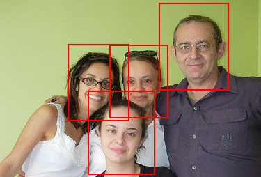
Fig. 1: Example of an image from which a bag of four instances (framed faces) is extracted, three of which are positive (female).

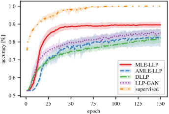
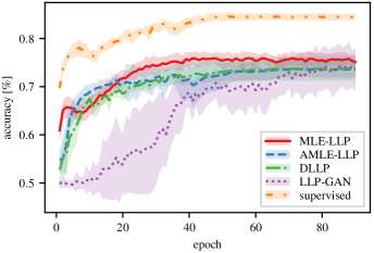
Fig. 2: Learning curves for the group photos (left) and CIFAR (right) datasets. The average test accuracy and the standard deviation is plotted using lines and error bands, respectively. One epoch corresponds to one pass of all training data through the network.

3 Experiments

We compare both MLE-LLP and AMLE-LLP with two existing deep LLP methods, DLLP [16] and LLP-GAN [17]. As a baseline, we use the standard supervised learning from all instance labels. All LLP methods were only provided with the number of positive instances in each bag. All experiment results were obtained via a 10-fold cross-validation.

The architecture in [17, Table 2 (CIFAR-10)] was used for LLP-GAN. The other methods employed the architecture from [17, Table 3 (CIFAR-10)]. The networks were trained via the Adam [21] optimizer. Image transformations (flipping, blurring, and color adjustments) were applied to prevent overfitting. The reported results were achieved with the best hyper-parameters discovered through grid-search for each method individually.

The experiments were implemented using PyTorch 1.10.0 with TorchVision 0.11.1 and Lightning 1.5.9 and performed on a server equipped with Intel Xeon Silver 4214R (2.40GHz) and NVIDIA GeForce RTX 2080 Ti.

3.1 Datasets

Two different datasets were used in the experiments. The first dataset, which deals with sex classification, is based on a real-world annotated dataset of family photos [22]. The annotations provide the position, sex, and age category of the faces in each image. We extracted the face regions (see Fig. 1), rescaled them to $72\times 90$ px, and kept only those of people older than 12 years. Faces in one image formed a bag. We omitted images containing more than 12 faces, resulting in ${1\,913}$ bags of ${3\,439}$ and $4\,012$ male and female instances, respectively. Using the LLP formulation is beneficial in this application, as it is faster for the annotator to count the number of males/females in the photo than manually select the respective faces.

The second dataset consisted of the bird and cat classes from the CIFAR-10 [23] dataset, a collection of $32\times 32$ px color images. Bags of uniform random sizes $n$, $1\leq n\leq 12$, were constructed by uniform random sampling without replacement.

Table 1: Average epoch duration ($\pm 1\sigma$). For MLE-LLP, the duration includes both the E and M steps.

	epoch duration [s]
method	group photos	CIFAR
MLE-LLP	$16.66\pm 0.25$	$7.78\pm 0.16$
AMLE-LLP	$29.33\pm 0.33$	$20.23\pm 0.20$
DLLP	$30.38\pm 0.31$	$18.66\pm 0.19$
LLP-GAN	$77.01\pm 0.78$	$51.20\pm 0.29$
supervised	$12.81\pm 0.19$	$3.65\pm 0.13$

3.2 Convergence

The first experiment focused on the convergence of the methods on both datasets. The average epoch time was measured, and the learning curves were plotted for all methods.

For both datasets, the supervised method converged to an accuracy that was $\approx 10\%$ higher than the LLP methods (see Fig. 2). On the group photos, MLE-LLP led steadily to a better performance than the competitors, while on CIFAR, the methods converged to a comparable accuracy. Furthermore, MLE-LLP exhibited lower variance of its performance than the other LLP methods.

Among the LLP methods, MLE-LLP was the most efficient in terms of time as it required significantly fewer epochs for convergence than the other LLP methods, including AMLE-LLP: approximately $3\times$ fewer for the group photos and $2\times$ for CIFAR. Moreover, one epoch of MLE-LLP was about twice as fast on average than for the other LLP methods (see Tab. 1). The speed was achieved mainly by processing the data in bigger batches, which MLE-LLP natively enables.

3.3 Bag size impact

We considered seven bag sizes $n\in\{2^{k}\mid k=1,\ldots,7\}$. For each bag size, we generated a dataset by randomly sampling instances from CIFAR-10 without replacement, creating bags of size $n$. MLE-LLP was tested only for small bag sizes where its computation requirements were reasonable.

Generally, the methods behave similarly. Their performance degrades as the bag size grows: the accuracy decreases by $\approx 5\%$ each time the bag size doubles. This follows from the fact that, as the bag size grows, the distribution of instance labels in a bag approaches their a priori distribution, which is uniform in this case, limiting the information available to LLP [15].

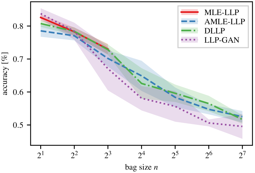
Fig. 3: Dependency of the performance of the LLP methods on the bag size.

4 Conclusion

This paper considered learning from label proportions (LLP) when the training dataset consists of small bags. Our MLE-LLP method is general, it can be used with any instance classifier. It considers all possible configurations consistent with the annotations, which allows for faster convergence than existing methods based on deep learning. Faster convergence is especially desirable when big datasets consisting of high-dimensional instances are processed. Unlike existing methods, MLE-LLP enables processing the data in arbitrarily-sized batches. The source code and the data is available online.

Acknowledgments

The authors acknowledge the support of the OP VVV funded project “CZ.02.1.01/0.0/0.0/16_019/0000765 Research Center for Informatics”, the Czech Science Foundation project 20-08452S, and the Grant Agency of the CTU in Prague, grant No. SGS20/170/OHK3/3T/13.

References

- [1] D. R. Musicant et al., “Supervised learning by training on aggregate outputs,” in Seventh IEEE International Conference on Data Mining. IEEE, 2007, pp. 252–261.
- [2] J. Hernández-González et al., “Fitting the data from embryo implantation prediction: Learning from label proportions,” Statistical methods in medical research, vol. 27, no. 4, pp. 1056–1066, 2018.
- [3] D. Baručić et al., “Automatic evaluation of human oocyte developmental potential from microscopy images,” in 17th International Symposium on Medical Information Processing and Analysis. 2021, vol. 12088 of Proceedings of SPIE, SPIE.
- [4] D. Habart et al., “Automated analysis of microscopic images of isolated pancreatic islets,” Cell transplantation, vol. 25, no. 12, pp. 2145–2156, 2016.
- [5] V. Lempitsky and A. Zisserman, “Learning to count objects in images,” Advances in neural information processing systems, vol. 23, pp. 1324–1332, 2010.
- [6] P. Bandi et al., “From detection of individual metastases to classification of lymph node status at the patient level: the CAMELYON17 challenge,” IEEE Transactions on Medical Imaging, vol. 38, no. 2, pp. 550–560, 2018.
- [7] G. Bortsova et al., “Deep learning from label proportions for emphysema quantification,” in International Conference on Medical Image Computing and Computer-Assisted Intervention. Springer, 2018, pp. 768–776.
- [8] Y. Ding et al., “Learning from label proportions for sar image classification,” Eurasip Journal on Advances in Signal Processing, vol. 2017, no. 1, pp. 1–12, 2017.
- [9] Stefan Rueping, “SVM classifier estimation from group probabilities,” in Proceedings of the 27th International Conference on Machine Learning, 2010, pp. 911–918.
- [10] K.-T. Lai et al., “Video event detection by inferring temporal instance labels,” in Proceedings of the IEEE Conference on Computer Vision and Pattern Recognition, 2014, pp. 2243–2250.
- [11] F. X. Yu et al., “Modeling attributes from category-attribute proportions,” in Proceedings of the 22nd ACM international conference on Multimedia, 2014, pp. 977–980.
- [12] G. Dulac-Arnold et al., “Deep multi-class learning from label proportions,” arXiv preprint arXiv:1905.12909, 2019.
- [13] Zhensong Chen et al., “Learning with label proportions based on nonparallel support vector machines,” Knowledge-Based Systems, vol. 119, pp. 126–141, 2017.
- [14] F. X. Yu et al., “SVM for learning with label proportions,” in Proceedings of the 30th International Conference on Machine Learning. 2013, vol. 28 of Proceedings of Machine Learning Research, pp. 504–512, PMLR.
- [15] F. X. Yu et al., “On learning from label proportions,” arXiv preprint arXiv:1402.5902, 2015.
- [16] E. M. Ardehaly and A. Culotta, “Co-training for demographic classification using deep learning from label proportions,” in 2017 IEEE International Conference on Data Mining Workshops. IEEE, 2017, pp. 1017–1024.
- [17] J. Liu et al., “Learning from label proportions with generative adversarial networks,” in Advances in Neural Information Processing Systems, 2019, pp. 7167–7177.
- [18] K-H. Tsai and H.-T. Lin, “Learning from label proportions with consistency regularization,” in Asian Conference on Machine Learning. PMLR, 2020, pp. 513–528.
- [19] B. Flach and V. Hlavac, Computer Vision: A Reference Guide, chapter Expectation Maximization Algorithm, pp. 265–268, Springer US, Boston, MA, 2014.
- [20] E. Rosenman and N. Viswanathan, “Using Poisson binomial GLMs to reveal voter preferences,” arXiv preprint arXiv:1802.01053, 2018.
- [21] D. P. Kingma and J. Ba, “Adam: A method for stochastic optimization,” in 3rd International Conference on Learning Representations, Yoshua Bengio and Yann LeCun, Eds., 2015.
- [22] A. Gallagher and T. Chen, “Understanding groups of images of people,” in IEEE Conference on Computer Vision and Pattern Recognition, 2009, pp. 256–263.
- [23] A. Krizhevsky, “Learning multiple layers of features from tiny images,” Tech. Rep., University of Toronto, 2009, https://www.cs.toronto.edu/~kriz/learning-features-2009-TR.pdf, accessed February 2022.