Efficient GPU implementation of randomized SVD and its applications
Abstract
Matrix decompositions are ubiquitous in machine learning, including applications in dimensionality reduction, data compression and deep learning algorithms. Typical solutions for matrix decompositions have polynomial complexity which significantly increases their computational cost and time. In this work, we leverage efficient processing operations that can be run in parallel on modern Graphical Processing Units (GPUs), predominant computing architecture used e.g. in deep learning, to reduce the computational burden of computing matrix decompositions. More specifically, we reformulate the randomized decomposition problem to incorporate fast matrix multiplication operations (BLAS-3) as building blocks. We show that this formulation, combined with fast random number generators, allows to fully exploit the potential of parallel processing implemented in GPUs. Our extensive evaluation confirms the superiority of this approach over the competing methods and we release the results of this research as a part of the official CUDA implementation111https://docs.nvidia.com/cuda/cusolver/index.html.
Keyword: Matrix decompositions, randomized SVD, eigenvalues, CUDA, GPU
1 Introduction
Matrix decomposition is a fundamental operation widely used across numerous real-life applications, including data compression, optimization of machine learning models and dimensionality reduction. The latter application remains especially challenging, given the increasing amount of real-world highly-dimensional data, such as multi-lingual textual corpora or drug discovery databases with complex chemical compounds. Although the original dimensionality of those datasets is high, in practice the data lays on lower-dimensional subspace with a smaller number of parameters. Dimensionaly reduction methods, such as singular value decomposition (SVD) [1], are typically used to find this lower-dimensional subspace in real-life problems ranging from data analysis [2, 3], data compression [4, 5], statistics and machine learning [6, 7] as well as clustering [8]. Despite the ubiquity of SVD, its computational complexity poses a significant problem, especially when dealing with large-scale datasets.
One of the approaches proposed to address this limitation of SVD is to approximate matrices of low rank using randomization techniques [9, 10]. These techniques are well known to give a significant speed-up, yet their practical implementations are often cumbersome and do not leverage recent advancements in the architectural design of contemporary computational hardware, such as Graphical Processing Units (GPUs). For instance, the baseline methods used to solve this task, such as GESVD or Krylov subspace methods [11], do not utilize computational linear algebra to parallelize the operations, and effectively reduce the computational cost of SVD.
In this work, we present a new approach towards solving randomized SVD problem efficiently by exploiting fast matrix multiplications and random number generators, implemented on contemporary GPUs. More specifically, we rely on the computational linear algebra to decompose randomized SVD into a set of low-level matrix multiplications known as Basic Linear Algebra Subprograms222BLAS functionality is categorized into three sets of routines called ”levels”: BLAS-1 operations typically take linear time , Bias-2 operations quadratic time, and BLAS-3 operations cubic time. (BLAS) [12]. These subprograms contain BLAS-1 and BLAS-2 operations, which are limited by system bandwidth, and BLAS-3 operations bounded by the arithmetic operation throughput of a machine. The key to achieving high performance matrices operations is the effective translation of the computations into a set of BLAS-3 operations, since those operations can be easily run in parallel on modern hardware architectures such as GPUs. This paper shows that such a solution can be efficiently implemented on the contermporary GPUs and allows for faster processing of large-scale dataset.
To confirm the efficacy of our method, we extensively evaluate our approach against the state-of-the-art competitors. Figure 1 shows the results of this evaluation which confirms the effectiveness of our implementation and a significant acceleration it obtains relative to state-of-the-art methods. In the presented experiment, we consider two types of methods that calculate the whole spectrum of eigenvalues such as GESVD GPU and LAPACK [13] dgesvd, as well as the methods that calculate only largest eigenvalues such as LAPACK dsyevr, randomized singular value decomposition (RSVD) [14] and SVDS from package [15]. As a dataset, we take CelebA [16] where we resize the images to different sizes and our approach shows consistent 10x speedup, cf. Section 4.
To summarize, our contributions can be defined as follows:
-
•
We introduce a novel approach for speeding up randomized SVD computations based on fast GPU operations: BLAS-2 matrix multiplications and random number generations.
-
•
We extensively evaluate our method against state-of-the-art approaches and empirically prove its improved efficacy.
-
•
We make our findings available to the public by releasing our code as part of the official CUDA implementation.
2 Related works
Principal component analysis (PCA) is commonly used for dimensionality reduction by projecting each data point onto only the first few principal components to obtain lower-dimensional data while preserving as much of the data’s variation as possible. It can be shown that the principal components are eigenvectors of the data’s covariance matrix. Thus, the principal components are often computed by eigendecomposition of the data covariance matrix or singular value decomposition (SVD) of the data matrix.
If the matrix is small, we can compute eigenvalues using the characteristic polynomial. In practice, eigenvalues of large matrices are not computed using the characteristic polynomial, and algorithms to find them are iterative. There are Iterative numerical algorithms for approximating roots of polynomials, such as Newton’s method, but, in general, it is impractical to compute the characteristic polynomial and then apply these methods. One reason is that small round-off errors in the coefficients of the characteristic polynomial can lead to large errors in the eigenvalues and eigenvectors [17].
One of the simplest and most accurate iterative algorithms is the power method [18] (also known as the Von Mises iteration). In this method, a given vector is repeatedly applied to a matrix and properly normalized. Consequently, it will lie in the direction of the eigenvector associated with the eigenvalues. The power iteration is simple, but it may converge slowly. Moreover, the method approximates only one eigenvalue of a matrix. The Power approach is usually used as a part of more efficient techniques, e.g. Krylov methods [11], inverse iteration, QR-method. The basis of the QR method for calculating the eigenvalues of is the fact that real matrix can be factorized as where is orthogonal and is upper triangular. The method is efficient for the calculation of all eigenvalues of a matrix.
In the case of a large data set, we do not usually require all the eigenvalues, but only a few first ones. Partial singular value decomposition algorithms are usually based on the Lanczos algorithm [19, 20, 21, 22]. Randomized matrix algorithms nowadays are most popular in practical applications. In [23] authors proposed Monte Carlo approach to SVD decomposition. The method for approximation of low-rank SVD decomposition is based on non-uniform row and column sampling. In [24, 25, 26] authors introduced a more robust approach based on random projections. The method constructs a subspace that captures the column space of a matrix. The modification of the method, which uses fast matrix multiplications was introduced in [27]. In [28] authors unified and expanded previous work on the randomized singular value decomposition and introduced state-of-the-art algorithms to compute the approximation of low-rank singular value decomposition.
The basic idea of probabilistic matrix algorithms is to apply a degree of randomness to derive a smaller matrix from a high-dimensional matrix, which captures the essential information. Then, a deterministic matrix factorization algorithm is applied to the smaller matrix to compute a near-optimal low-rank approximation. Recent has been demonstrated that this probabilistic framework can be effectively used to compute the pivoted QR decomposition [29], the pivoted LU decomposition [30].
3 Method description
In this section, we define the problem and introduce our method that leverages GPU computations of probabilistic matrix operations to speed up the processing time.
First, let be an arbitrary matrix for any , and be the target number of singular values. Recall that making singular value decomposition (SVD) of we obtain
where , are orthogonal matrices for . The above decomposition of is called as the compact SVD while it is a simple transformation of a classical SVD decomposition
where , are unitary and , have orthonormal columns.
In our approach, we use the randomized SVD algorithm as it is a straightforward realization of the proposed randomized SVD code from [28], which computes the -SVD of up to Frobenius norm relative error. Let be a good sketch of , the column space of should roughly contain the columns of by the low-rank approximation property i.e.
where is Frobenius norm and . If is a Gaussian projection matrix [31] or count sketch [32] and 333The notation defines the asymptotic behavior., then the low-rank approximation property
holds in expectation.
From the above property we can describe randomized -SVD pseudo-algorithm in the several steps that are described in Algorithm 1.
Note that so if you want only -th largest eigenvalues of matrix , we used only the first five points of the Algorithm 1 procedure, i.e. we needed only the matrix . In Section 4 we describe and show results of experiments, where we calculate only -th largest eigenvalues.
GPU computations to speed up processing
The above formulation let us decompose the problem of SVD into a set of matrix operations (predominantly multiplications) with a significant number of random numbers induced by the probabilistic approach. Exactly those two features of our formulation lead to a significant speed up observed when implementing Algorithm 1 on modern GPU architectures.
Thanks to the parallel nature of GPU processing, matrix-matrix operations can be effectively computed using BLAS-3 operations. Throughput-oriented processors, such as GPUs, are especially well suited for this kind of operation. BLAS-3 kernels break down linear algebra operations in terms of GEMM-like operations, which attain very high performance on graphic processors.
Moreover, random number generators effectively optimized for GPU architecture can offer up to threefold speedup in processing time thanks to the CuRAND library555https://developer.nvidia.com/curand. Combined with the decomposition of randomized SVD into a set of matrix-matrix multiplications our approach leads to a significant computation speedups, as we present in the following sections.
4 Experiments
In this section, we evaluate the performance of our approach and compare it to other methods available either in CPU or in GPU. We document three different experiments: in the first one, we consider matrix A that is not square, then we test application of randomized SVD to principal component analysis of a random matrix, and finally we use our method to practical method of subspace clustering [8].
In the first two experiments, we run every method 10 times on the same datasets and calculate for average time denoted by and standard deviation denotes by . In the Figures we use the solid lines to draw the ratio , the dashed black line has a value of 1 (a reference to our method), and the shaded region of error defined by interval:
where denotes another method.
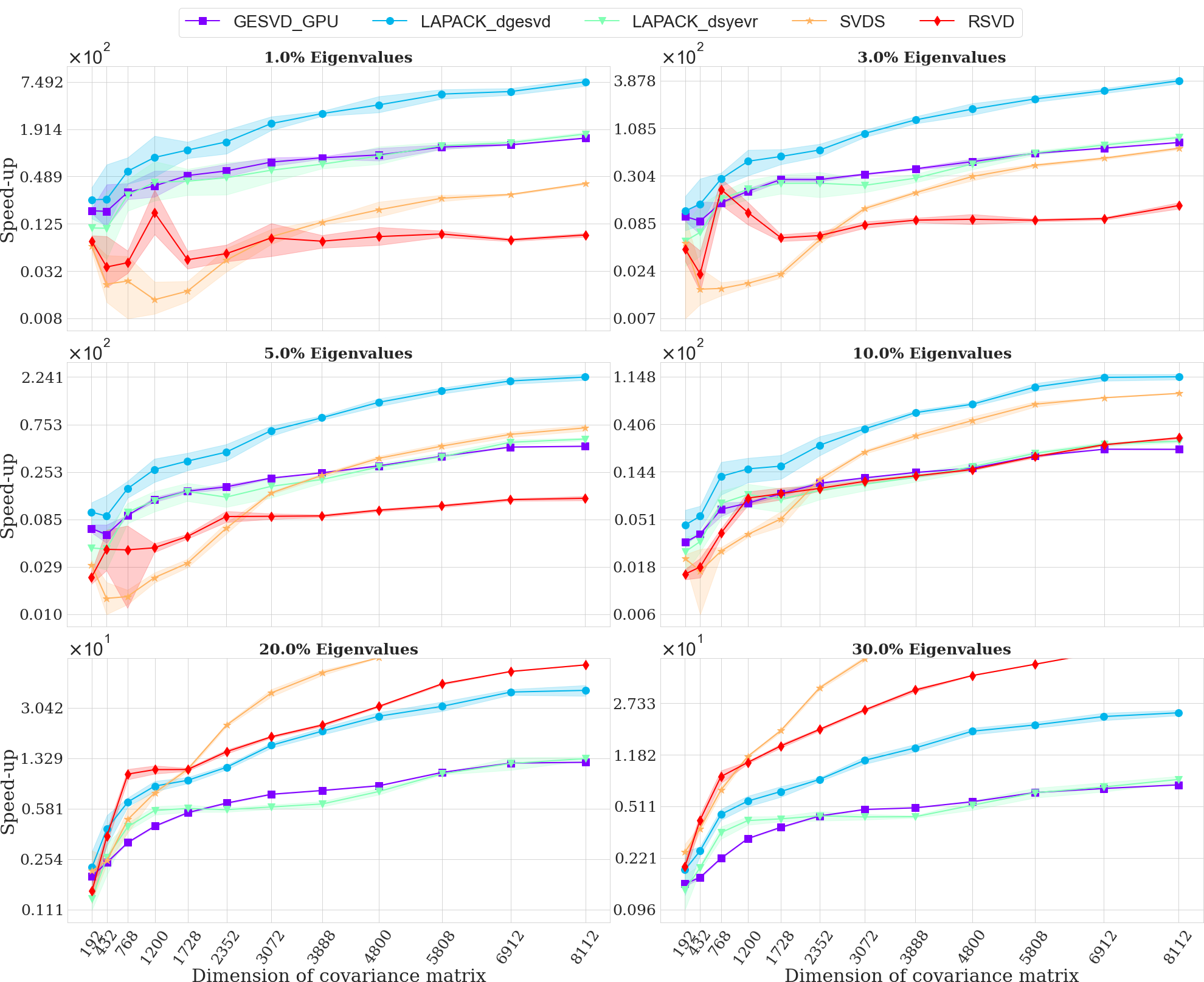
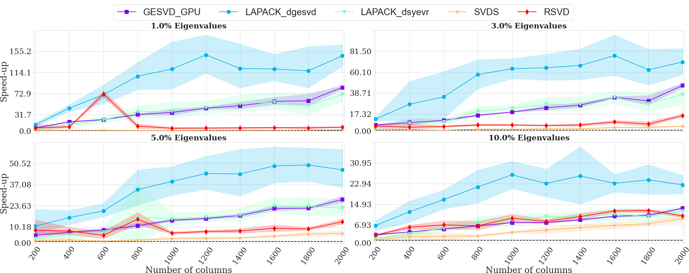
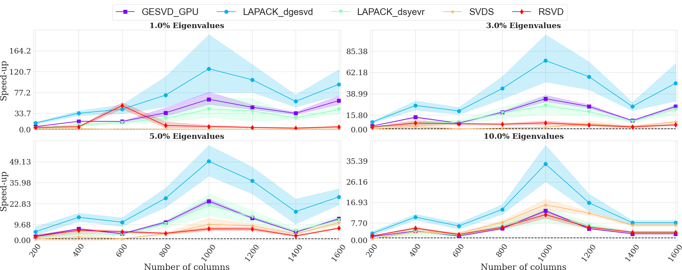
We consider two types of methods that calculate the whole spectrum such as GESVD GPU and LAPACK [13] dgesvd and methods that calculate only largest eigenvalues such as LAPACK dsyevr, randomized singular value decomposition (RSVD) [14] and SVDS from package [15].
Performance comparison
In this experiment, we make three different test cases for which we construct the matrix for with random orthogonal matrices and a certain spectrum , where for and
-
(i)
— fast decay,
-
(ii)
— sharp decay (around breakout point ),
-
(iii)
— slow decay.
We take 1%, 3%, 5%, 10% of eigenvalues on matrix sizes i.e. for 5% we calculate the largest eigenvalues. Due to the randomized singular value decomposition in our calculation, we kept the relative error on the limit of at most against the baseline method, which is GESVD GPU. Figures 2, 3, 4 show the evaluation results. The dashed black line has a value of 1 (a reference to our method).
Application to Principal Component Analysis
Principal Component Analysis (PCA) is a well-established technique for dimensionality reduction and multivariate analysis. Examples of its many applications include data compression, image processing, visualization, exploratory data analysis, pattern recognition, and time series prediction.
PCA is related to eigenvectors and eigenvalues because with their help we can reduce the dimensionality of the data at a certain level of information preservation in the data. The eigenvectors of the covariance matrix of data are actually the directions of the axes where there is the most variance (most information) and that we call Principal Components. On the other hence, the eigenvalues are simply the coefficients attached to eigenvectors, which give the amount of variance carried in each Principal Component.
In this example, we compare a few state-of-the-art numerical methods to solve the eigenproblem. We consider not only the methods that can calculate the whole spectrum and associate with their eigenvalues. In particular, we focus on ones that can calculate only several eigenvalues, because our interest-only largest eigenvalues, i.e. we want to calculate only Principal Components. Figure 1 shows the time of operation of other methods in relation to ours (speed-up). As a dataset, we take CelebA [16] where we resize the images to sizes , , , . Each RGB image about size , we flatten to the vector with size , where , is height, and the width of the image, respectively.
Application for subspace clustering
Subspace clustering is one of the applications of the singular value decomposition of the matrices. In this part of the paper we present the results of comparison of the method SuMC that is presented in [8] and application of this code with the randomized SVD algorithm that requires minor changes in the code.
| Dataset | Solver type | Elapsed time (sec) | Solver calls | ARI score |
|---|---|---|---|---|
| first | CPU | 73653.0 | 262209 | 1.0 |
| GPU | 2584.5 | 189291 | 1.0 | |
| \cdashline2-5[4pt/3pt] second | CPU | - | - | - |
| GPU | 23967.0 | 1944144 | 1.0 |
Table 4 shows the results of method of SuMC which used solver of eigenvalues implemented on CPU and GPU in synthetic datasets, which we randomly generate on the spaces , where dim denotes dimension of a space. In these generated data we known upfront what are the real subspaces and we can use the theoretical compression rate for the data set. We generate 2 random synthetic datasets: the first contained points from -dimensional subspace, points from -dimensional subspace and points from -dimensional subspace, where each points were presented in -dimensional space; the second data contained points from -dimensional subspace, points from -dimensional subspace and points from -dimensional subspace (each points were described in -dimensional space), and for them, we calculated the mean of Rand index adjusted. In each experiment we started with the same initialization of points to clusters.
Note that the number of the solver call is the case of GPU in smaller than CPU which may indicate better generalization and this in turn result in faster convergence of the SuMC algorithm.
5 Conclusion
The experiments confirmed practical usability and high performance of the GPU implementation of a randomized SVD algorithm for computing small part of the spectrum. We have tested the method in three different tasks, i.e. just the performance analysis to compute 1-10% of the spectrum, application for PCA, and application for subspace clustering. Obtained results were satisfactory across the board, with the speedup reaching up to 100x for some chosen cases. Be believe that applying this method for large scale PCA, as part of the machine learning pipeline might be instrumental.
Acknowledgments
The authors would like to thank Lung Sheng Chien for discussion and comments on the paper. This research was supported by: grant no POIR.04.04.00-00-14DE/18-00 carried out within the Team-Net program of the Foundation for Polish Science co-financed by the European Union under the European Regional Development Fund. This research was funded in part by National Science Centre, Poland grant no. 2020/39/D/ST6/01332 and grant no. 2020/39/B/ST6/01511. For the purpose of Open Access, the authors have applied a CC-BY public copyright licence to any Author Accepted Manuscript (AAM) version arising from this submission.
References
- [1] Michael E Wall, Andreas Rechtsteiner, and Luis M Rocha. Singular value decomposition and principal component analysis. In A practical approach to microarray data analysis, pages 91–109. Springer, 2003.
- [2] Steven Ding, Ping Zhang, Eve Ding, Amol Naik, Pengcheng Deng, and Weihua Gui. On the application of pca technique to fault diagnosis. Tsinghua Science and Technology, 15(2):138–144, 2010.
- [3] Mohamed-Faouzi Harkat, Gilles Mourot, and José Ragot. An improved pca scheme for sensor fdi: Application to an air quality monitoring network. Journal of Process Control, 16(6):625–634, 2006.
- [4] R Dony et al. Karhunen-loeve transform. The transform and data compression handbook, 1:1–34, 2001.
- [5] Michael Gastpar, Pier Luigi Dragotti, and Martin Vetterli. The distributed karhunen–loeve transform. IEEE Transactions on Information Theory, 52(12):5177–5196, 2006.
- [6] Weihua Li, H Henry Yue, Sergio Valle-Cervantes, and S Joe Qin. Recursive pca for adaptive process monitoring. Journal of process control, 10(5):471–486, 2000.
- [7] Heiko Hoffmann. Kernel pca for novelty detection. Pattern recognition, 40(3):863–874, 2007.
- [8] Łukasz Struski, Jacek Tabor, and Przemysław Spurek. Lossy compression approach to subspace clustering. Information Sciences, 435:161 – 183, 2018.
- [9] Xu Feng, Wenjian Yu, and Yaohang Li. Faster matrix completion using randomized svd. In 2018 IEEE 30th International Conference on Tools with Artificial Intelligence (ICTAI), pages 608–615. IEEE, 2018.
- [10] Vicente E Oropeza and Mauricio D Sacchi. A randomized svd for multichannel singular spectrum analysis (mssa) noise attenuation. In SEG Technical Program Expanded Abstracts 2010, pages 3539–3544. Society of Exploration Geophysicists, 2010.
- [11] Aleksej Nikolajevic Krylov. O cislennom resenii uravnenija, kotorym v techniceskih voprasah opredeljajutsja castoty malyh kolebanii material’nyh sistem. Izv. Akad. Nauk SSSR. Ser. Fiz.-Mat, 4:491–539, 1931.
- [12] Chuck L Lawson, Richard J. Hanson, David R Kincaid, and Fred T. Krogh. Basic linear algebra subprograms for fortran usage. ACM Transactions on Mathematical Software (TOMS), 5(3):308–323, 1979.
- [13] Edward Anderson, Zhaojun Bai, Christian Bischof, L Susan Blackford, James Demmel, Jack Dongarra, Jeremy Du Croz, Anne Greenbaum, Sven Hammarling, Alan McKenney, et al. LAPACK users’ guide. SIAM, 1999.
- [14] N. Benjamin Erichson. Randomized singular value decomposition. https://CRAN.R-project.org/package=rsvd, 2020.
- [15] Qiu Yixuan, Mei Jiali, Guennebaud Gael, and Niesen Jitse. Solvers for large-scale eigenvalue and svd problems. https://CRAN.R-project.org/package=RSpectra, 2019.
- [16] Ziwei Liu, Ping Luo, Xiaogang Wang, and Xiaoou Tang. Deep learning face attributes in the wild. In Proceedings of International Conference on Computer Vision (ICCV), December 2015.
- [17] Lloyd N Trefethen and David Bau III. Numerical linear algebra, volume 50. Siam, 1997.
- [18] RV Mises and Hilda Pollaczek-Geiringer. Praktische verfahren der gleichungsauflösung. ZAMM-Journal of Applied Mathematics and Mechanics/Zeitschrift für Angewandte Mathematik und Mechanik, 9(1):58–77, 1929.
- [19] Daniela Calvetti, Lothar Reichel, and Danny Chris Sorensen. An implicitly restarted lanczos method for large symmetric eigenvalue problems. Electronic Transactions on Numerical Analysis, 2(1):21, 1994.
- [20] Rasmus Munk Larsen. Lanczos bidiagonalization with partial reorthogonalization. DAIMI Report Series, (537), 1998.
- [21] Richard B Lehoucq, Danny C Sorensen, and Chao Yang. ARPACK users’ guide: solution of large-scale eigenvalue problems with implicitly restarted Arnoldi methods. SIAM, 1998.
- [22] James Baglama and Lothar Reichel. Augmented implicitly restarted lanczos bidiagonalization methods. SIAM Journal on Scientific Computing, 27(1):19–42, 2005.
- [23] Alan Frieze, Ravi Kannan, and Santosh Vempala. Fast monte-carlo algorithms for finding low-rank approximations. Journal of the ACM (JACM), 51(6):1025–1041, 2004.
- [24] Tamas Sarlos. Improved approximation algorithms for large matrices via random projections. In 2006 47th Annual IEEE Symposium on Foundations of Computer Science (FOCS’06), pages 143–152. IEEE, 2006.
- [25] Edo Liberty, Franco Woolfe, Per-Gunnar Martinsson, Vladimir Rokhlin, and Mark Tygert. Randomized algorithms for the low-rank approximation of matrices. Proceedings of the National Academy of Sciences, 104(51):20167–20172, 2007.
- [26] Per-Gunnar Martinsson, Vladimir Rokhlin, and Mark Tygert. A randomized algorithm for the decomposition of matrices. Applied and Computational Harmonic Analysis, 30(1):47–68, 2011.
- [27] Franco Woolfe, Edo Liberty, Vladimir Rokhlin, and Mark Tygert. A fast randomized algorithm for the approximation of matrices. Applied and Computational Harmonic Analysis, 25(3):335–366, 2008.
- [28] Nathan Halko, Per Gunnar Martinsson, and Joel A Tropp. Finding structure with randomness: Probabilistic algorithms for constructing approximate matrix decompositions. SIAM review, 53(2):217–288, 2011.
- [29] Jed A Duersch and Ming Gu. Randomized qr with column pivoting. SIAM Journal on Scientific Computing, 39(4):C263–C291, 2017.
- [30] Gil Shabat, Yaniv Shmueli, Yariv Aizenbud, and Amir Averbuch. Randomized lu decomposition. Applied and Computational Harmonic Analysis, 44(2):246–272, 2018.
- [31] William B Johnson and Joram Lindenstrauss. Extensions of lipschitz mappings into a hilbert space. Contemporary mathematics, 26(189-206):1, 1984.
- [32] Moses Charikar, Kevin Chen, and Martin Farach-Colton. Finding frequent items in data streams. In International Colloquium on Automata, Languages, and Programming, pages 693–703. Springer, 2002.