The muon $g-2$ with four flavors of staggered quarks

Abstract

We present updated results for the light-quark connected part of the leading hadronic contribution to the muon $g-2$ from configurations with 2+1+1 flavors of HISQ quarks using the time-momentum representation of the electromagnetic current correlator. We have added statistics on two ensembles as well as a fourth lattice spacing using configurations that have been generated by the MILC collaboration at the physical pion mass. Additionally we account for the leading finite-volume and taste-breaking effects using Staggered Chiral Perturbation Theory at NNLO.

1 Introduction

The muon anomalous magnetic moment $a_{\mu}=(g-2)/2$ has become a leading candidate quantity with which to test the Standard Model. The latest experimental result from Fermilab this past April [1], when combined with the previous result from Brookhaven [2], now shows a 4.2$\sigma$ deviation from the Standard Model prediction (for a summary of the results from the $g-2$ theory initiative, both from phenomenology and the lattice, see Ref. [3]). The BMW collaboration recently found a smaller discrepancy with experiment, $1.5\sigma$ [4], when their sub-percent lattice QCD value for the HVP contribution is used instead of the data-driven value from the Muon g-2 Theory Initiative [3]. The uncertainty in the Fermilab result will only decrease in the next couple of years, and it is important for the Standard Model calculation, which until recently has primarily come from the dispersive estimate, to keep pace.

It has become increasingly clear that a first-principles approach to determining the QCD contributions using lattice calculations is possible, given improvements in simulations during the last ten to fifteen years. Improving statistics on the lattice data is crucial of course, but also correcting for the many systematics is necessary to produce a reliable result.

We provide an update on our previous results [5, 6] for the leading hadronic contribution to the muon $g-2$ (coming from the light quarks only), with a continuing focus on the systematics that arise when using staggered quarks in a finite volume. To do so, we have calculated the finite-volume and taste-breaking effects to next-to-next-to leading order (NNLO) in staggered chiral perturbation theory (ChPT).

2 Simulation details

We obtain the leading hadronic contribution to the muon $g-2$ from the expression

$$a_{\mu}^{\rm HVP}=4\alpha^{2}\int_{0}^{\infty}dq^{2}f(q^{2})\hat{\Pi}(q^{2}),$$ (1)

where $f(q^{2})$ is the kernel defined in Ref. [7], and $\hat{\Pi}(q^{2})\equiv\Pi(0)-\Pi(q^{2})$ is the subtracted hadronic vacuum polarization, coming from the Fourier transform of the vector two-point function (we use the conserved vector current in our calculation). As is common with current lattice calcuations, we use the time-momentum representation [8],

$$\Pi(0)-\Pi(q^{2})=\sum_{t}\left(\frac{\cos{qt}-1}{q^{2}}+\frac{1}{2}t^{2}\right)C(t),\quad C(t)=\frac{1}{3}\sum_{\vec{x},i}\langle j^{i}(\vec{x},t)j^{i}(0)\rangle,$$ (2)

where $C(t)$ is the Euclidean time correlation function, averaged over spatial directions. Equation (1) becomes $a_{\mu}^{\rm HVP}(T)=2\sum_{t=0}^{T/2}w(t)C(t)$, with the weight

$$w(t)=4\alpha^{2}\int_{0}^{\infty}{d\omega^{2}}f(\omega^{2})\left[\frac{\cos{\omega t}-1}{\omega^{2}}+\frac{t^{2}}{2}\right].$$ (3)

To reduce noise in our results, we use a combination of full volume low-mode averaging and all-mode averaging, to calculate the correlator in Eq. (2) [9, 10, 11, 12]. While we do not include the details of this implementation here, they are discussed in Ref. [5].

$m_{\pi}\ ({\rm MeV})$	$a\ ({\rm fm})$	$L^{3}$	$L\ ({\rm fm})$	$m_{\pi}L$	LM	# confs	traj. sep.
133	0.15148(80)	$32^{3}$	4.83	3.26	8000	48	40
130	0.08787(46)	$64^{3}$	5.62	3.66	8000	38	100
134	0.05684(30)	$96^{3}$	5.46	3.73	8000	35	60

Table 1: Lattice simulation details for the additional results for our calculation.

We use configurations generated by the MILC Collaboration [13] with 2+1+1 flavors of HISQ quarks. The new data comes from the configurations shown in Table 1, which we compare to our older results (not shown here, but they are shown in Ref. [5]). We have new computations on the two finest lattice spacings ($a\approx 0.06$ and 0.09 fm), and have added the coarser $a\approx 0.15$ fm lattice spacing, all near the physical pion mass. All but the coarsest lattice spacing have a spatial volume of around $(5.5~{}\rm{fm})^{3}$ (the $a=0.15$ fm ensemble has $L^{3}\sim(4.83~{}{\rm fm})^{3}$), and $m_{\pi}L\approx 3.3-3.7$. For all of the newer results, we use 8000 low modes (as opposed to either 4000 or 6000 low modes in our original results), and we separate our lattices by 40-100 trajectories as opposed to 12-48 in our original results.

3 Finite-volume chiral perturbation theory

In order to study the leading staggered taste-breaking effects we calculate the vector correlator to two loops (NNLO) in staggered ChPT [14, 15]. In our earlier result [5, 6], we used a hybrid approach: we calculated the one-loop corrections in staggered ChPT, extrapolated to the continuum, then applied the two-loop continuum finite volume corrections. Here however, we perform the full staggered ChPT calculation (in Euclidean space) at two loops as was done by the BMW collaboration [4].

After a straightforward (albeit lengthy) calculation, we obtain at NNLO,

$$C(t) = \frac{1}{48L^{3}}\sum_{\vec{p}}\sum_{X}\frac{{\vec{p}}^{2}}{E^{2}_{X}(p)}\,e^{-2E_{X}(p)t}\Biggl{(}1-\frac{1}{4f^{2}}\sum_{Y}D_{Y}(0)-\frac{16\ell_{6}(\vec{p}^{2}+m_{X}^{2})}{f^{2}}$$ (4)

$$+\frac{1}{24f^{2}}\,\frac{1}{L^{3}}\sum_{\vec{q}}\sum_{Y}\frac{{\vec{q}}^{2}}{E_{Y}(q)}\,\frac{1}{\vec{q}^{2}-\vec{p}^{2}+m_{Y}^{2}-m_{X}^{2}}\Biggr{)},$$

where the sums over $X$ and $Y$ run over the 16 pion tastes for staggered quarks, and

$$D_{Y}(0)=\frac{1}{L^{3}}\sum_{\vec{k}}\frac{1}{2E_{Y}(k)},\qquad E_{Y}(k)=\sqrt{k^{2}+m_{Y}^{2}}.$$ (5)

The sums over $\vec{p}$ and $\vec{k}$ are over the momenta $2\pi{\vec{n}}/L$ with ${\vec{n}}$ a three-vector of integers in a box with periodic boundary conditions. We define the renormalized $\ell_{6}^{r}$ by

$$\ell_{6}=\ell_{6}^{r}(\mu)-\frac{1}{3}\,\frac{1}{16\pi^{2}}\left(\frac{1}{\epsilon}-\log\mu-\frac{1}{2}(\log{(4\pi)}-\gamma+1)\right)\ .$$ (6)

In order to extract the finite-volume difference between the infinite-volume result for $a_{\mu}^{\rm HVP}$ and the finite-volume result, $\Delta a_{\mu}^{\rm HVP}=\left[\lim_{L\to\infty}a_{\mu}^{\rm HVP}(L)\right]-a_{\mu}^{\rm HVP}(L)$ in ChPT, we apply the Poisson Summation formula to Eq. (4). The resulting difference $\Delta a_{\mu}^{\rm HVP}$ follows, and after some simplification we perform the sums and integrals numerically.

With the parameters for our ensembles, we have calculated $\Delta a_{\mu}^{\rm HVP}$ both for the full result, as well as for the intermediate window method [12] where we have

$$a_{\mu}^{\rm HVP,win} = 2\sum_{t=0}^{T/2}C(t)w(t)(\Theta(t,t_{0},\Delta)-\Theta(t,t_{1},\Delta)),$$ (7)

$$\Theta(t,t^{\prime},\Delta) = \frac{1}{2}(1+\tanh((t-t^{\prime})/\Delta)),$$ (8)

with $t_{0}=0.4$ fm, $t_{1}=1.0$ fm, and $\Delta=0.15$ fm, as this allows us to compare with other lattice results. We show $\Delta a_{\mu}^{\rm HVP,win}\times 10^{10}$ for the window method in Table 2 for each of our ensembles (only at NLO), where we breakdown the finite-volume corrections due to the taste-pseudoscalar pion mass, the additional corrections that arise from staggered taste breaking, a correction needed to account for retuning the pion mass, and the final column is the total correction (from summing the previous three columns). We have the full NNLO corrections for the entire momentum range, however the numerical corrections for the window are more complicated to evaluate, so these were not included in this update.

			$m_{\pi_{5}}$	taste-breaking	$m_{\pi}$
$a$ (fm)	Volume	$m_{\pi_{5}}{\rm(MeV)}$	FV corr.	in FV	retuning	total
0.05684	$96^{3}$	134	0.727538	0.759853	-0.0687552	1.4186
0.08787	$64^{3}$	130	0.697276	3.51669	-0.516077	3.6979
0.12121	$48^{3}$	133	0.560572	7.99304	-0.21689	8.3367
0.15148	$32^{3}$	133	1.24171	10.3470	-0.186605	11.4021

Table 2: The various corrections $\Delta a_{\mu}^{\rm HVP,win}\times 10^{10}$ for the intermediate window at NLO from various sources: finite-volume effects due to the taste-pseudoscalar pion mass, additional corrections from staggered taste breaking, a correction need to retune the pion mass, and the total corrections (respectively).

4 Results & Conclusions

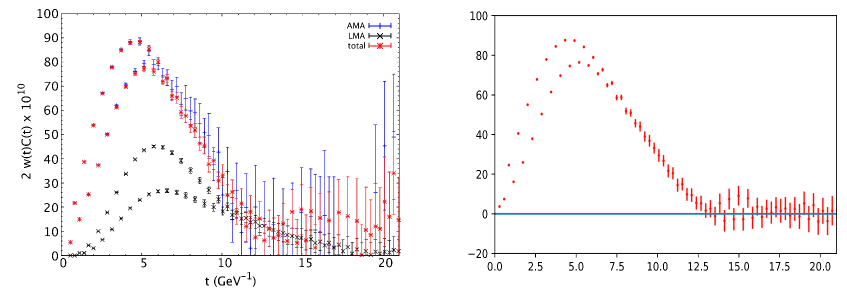
Figure 1: A comparison of the summand for our original data vs. new data for the $96^{3}$ ensemble.

For the $96^{3}$ ensemble, we compare our older results for the summand to the newer results in Fig. 1. On the left is the old data with 23 configurations and 4000 low modes (in red is the total result, combining the LMA and AMA results), and on the right is the new data with 35 configurations and 8000 low modes. One can see the marked reduction in error bars with the new data.

To extract $a_{\mu}^{\rm HVP}$ from our data more precisely, we use the bounding method of Refs. [12, 16]. We set bounds on the correlator for when $t$ is greater than a time $T$: $0<C(t)<C(T)e^{-E_{0}(t-T)}$, where $E_{0}=\infty$ (lower bound) or $2\sqrt{m_{\pi}^{2}+(2\pi/L)^{2}}$ (upper bound). At sufficiently large $T$ the bounds overlap, and an estimate for $a_{\mu}$ can be made which is more precise than simply summing over the noisy long-distance tail.

We show in Fig. 2 the extracted results for $a_{\mu}^{\rm HVP}$ using the bounding method. In Fig. 2(a) we directly compare the old and new data, while in Fig. 2(b) we compare the uncorrected and corrected new results. Note, the $a=0.12$ fm results are not new results, but are included in the fits, so we include that data point in the figure. The scaling behavior of the uncorrected data is quite different than that of the corrected data: the overall slope as $a^{2}\to 0$ changes sign between the two, and the uncorrected data exhibits a kink between large and small lattice spacings.

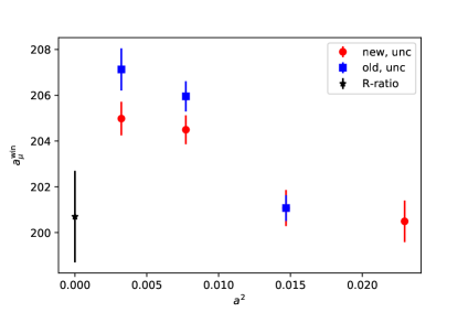
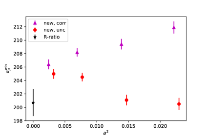
(a)                                                                   (b)

Figure 2: (a) A comparison of our old (circles) and new (squares) uncorrected results. (b) A comparison of the new uncorrected (circles) and new corrected (triangles) results.

In Fig. 3, we show various fits to the data. First we compare the original, uncorrected data to the corrected data in Fig. 3(a) with a simple linear fit in $a^{2}$. The extrapolated results for both fits are quite consistent, but the $\chi^{2}/$d.o.f. for the fit to the corrected data is better. In either case, the extrapolated result is not consistent with the $R$-ratio (for this value we use the result in our earlier work [5]). To check if our results could be consistent with the $R$-ratio determination, we perform several fits with that as a data point. Figs. 3(b) & (c) are quadratic fits in $a^{2}$, with and without the coarsest lattice spacing ($a\approx 0.15$ fm), while Fig. 3(d) is a fit inspired by perturbation theory [17], with a logarithm term: $A+Ba^{2}+Ca^{2}\log a^{2}$. Each of these fits have a reasonable $\chi^{2}/$d.o.f., and may indicate that the lattice data is not inconsistent with the $R$-ratio.

Our preliminary results suggest that simulations at even finer lattice spacings may be needed to determine whether the $R$-ratio and the lattice value are consistent. Additionally, finer lattice spacings can help understand the cutoff effects (the odd behavior of the uncorrected data is evidence for this). Currently we are running on a larger $a\approx 0.15$ fm ensemble (with $L=48$ instead of $L=32$) to help get a better handle on the finite volume effects.

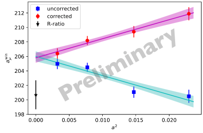
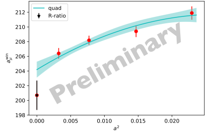
(a)                                                                   (b)

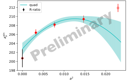
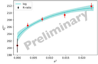
(c)                                                                   (d)

Figure 3: Various fits to the updated data. (a) compares a linear fit to the uncorrected and corrected data, while the other fits are only to corrected data, with (b) a quadratic fit to all lattice points but not the $R$-ratio, (c) a quadratic fit to all but the coarsest lattice point + the $R$-ratio point, and (d) a perturbation-theory-inspired fit to all points (including the $R$-ratio).

References

- [1] Muon Collaboration, B. Abi et. al., Measurement of the positive muon anomalous magnetic moment to 0.46 ppm, Phys. Rev. Lett. 126 (Apr, 2021) 141801.
- [2] Muon Collaboration, G. Bennett et. al., Final Report of the Muon E821 Anomalous Magnetic Moment Measurement at BNL, Phys.Rev. D73 (2006) 072003.
- [3] T. Aoyama et. al., The anomalous magnetic moment of the muon in the standard model, Physics Reports 887 (2020) 1–166.
- [4] S. Borsanyi, Z. Fodor, J. N. Guenther, C. Hoelbling, S. D. Katz, L. Lellouch, T. Lippert, K. Miura, L. Parato, K. K. Szabo, and et al., Leading hadronic contribution to the muon magnetic moment from lattice qcd, Nature 593 (Apr, 2021) 51–55, [arXiv:2002.1234].
- [5] C. Aubin, T. Blum, C. Tu, M. Golterman, C. Jung, and S. Peris, Light quark vacuum polarization at the physical point and contribution to the muon , Phys. Rev. D 101 (2020), no. 1 014503, [arXiv:1905.0930].
- [6] C. Aubin, T. Blum, M. Golterman, C. Jung, S. Peris, and C. Tu, Hadronic vacuum polarization in finite volume using NNLO ChPT, PoS LATTICE2019 (2019) 102, [arXiv:1910.0509].
- [7] T. Blum, Lattice calculation of the lowest order hadronic contribution to the muon anomalous magnetic moment, Phys.Rev.Lett. 91 (2003) 052001.
- [8] D. Bernecker and H. B. Meyer, Vector Correlators in Lattice QCD: Methods and applications, Eur.Phys.J. A47 (2011) 148.
- [9] L. Giusti, P. Hernandez, M. Laine, P. Weisz, and H. Wittig, Low-energy couplings of QCD from current correlators near the chiral limit, Journal of High Energy Physics 2004 (apr, 2004) 013–013.
- [10] T. DeGrand and S. Schaefer, Improving meson two-point functions in lattice qcd, Computer Physics Communications 159 (2004), no. 3 185–191.
- [11] T. Blum, T. Izubuchi, and E. Shintani, New class of variance-reduction techniques using lattice symmetries, Phys.Rev. D88 (2013) 094503.
- [12] RBC, UKQCD Collaboration, T. Blum et. al., Calculation of the hadronic vacuum polarization contribution to the muon anomalous magnetic moment, Phys. Rev. Lett. 121 (2018), no. 2 022003.
- [13] Fermilab Lattice, MILC Collaboration, A. Bazavov et. al., Charmed and light pseudoscalar meson decay constants from four-flavor lattice QCD with physical light quarks, Phys. Rev. D90 (2014), no. 7 074509.
- [14] C. Aubin and C. Bernard, Pion and kaon masses in staggered chiral perturbation theory, Phys. Rev. D68 (2003) 034014.
- [15] C. Aubin, T. Blum, M. Golterman, and S. Peris, Application of effective field theory to finite-volume effects in , Phys. Rev. D 102 (2020), no. 9 094511, [arXiv:2008.0380].
- [16] BMW Collaboration, S. Borsanyi et. al., Hadronic vacuum polarization contribution to the anomalous magnetic moments of leptons from first principles, Phys. Rev. Lett. 121 (2018), no. 2 022002.
- [17] N. Husung, P. Marquard, and R. Sommer, Asymptotic behavior of cutoff effects in Yang–Mills theory and in Wilson’s lattice QCD, Eur. Phys. J. C 80 (2020), no. 3 200, [arXiv:1912.0849].